A Review of Equation of State Models, Chemical Equilibrium Calculations and CERV Code Requirements for SHS Detonation Modelling
←
→
Page content transcription
If your browser does not render page correctly, please read the page content below
Defence Research and        Recherche et développement
Development Canada          pour la défense Canada

A Review of Equation of State Models,
Chemical Equilibrium Calculations and
CERV Code Requirements for SHS
Detonation Modelling

P. Thibault
TimeScales Scientific Ltd

Contract Scientific Authority: J. Lee, DRDC Suffield

The scientific or technical validity of this Contract Report is entirely the responsibility of the contractor and the contents
do not necessarily have the approval or endorsement of Defence R&D Canada.

                                    Defence R&D Canada
                                              Contract Report
                                    DRDC Suffield CR 2010-013
                                                October 2009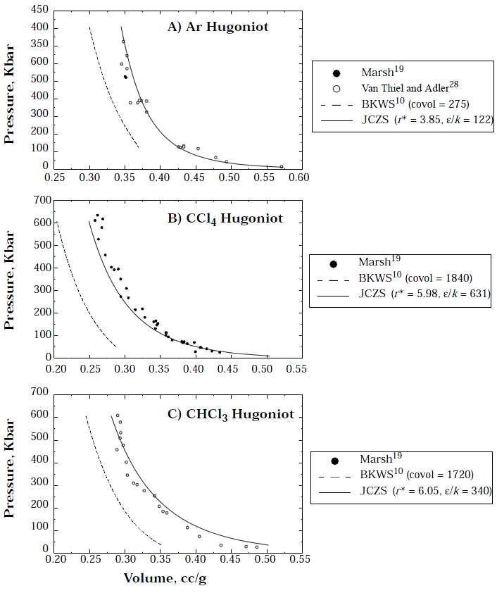
A Review of Equation of State Models,
Chemical Equilibrium Calculations and
CERV Code Requirements for SHS
Detonation Modelling

P. Thibault
TimeScales Scientific Ltd
554 Aberdeen Street SE
Medicine Hat AB T1A 0R7

Contract Number: Subcontract under W7702-08R183/001/EDM

Contract Scientific Authority: J. Lee (403-544-5025)

The scientific or technical validity of this Contract Report is entirely the responsibility of the contractor and the
contents do not necessarily have the approval or endorsement of Defence R&D Canada.

Defence R&D Canada – Suffield
Contract Report
DRDC Suffield CR 2010-013
October 2009
© Her Majesty the Queen as represented by the Minister of National Defence, 2009

© Sa majesté la reine, représentée par le ministre de la Défense nationale, 2009
ǡ
Paul Thibault
8 October 2009
WorkperformedforDRDCSuffieldundercontracttoUTIAS
TimeScalesScientificLtd.
1

TableofContents

Table of Contents.......................................................................................................................... 1
1. Introduction ............................................................................................................................... 3
2. Current Capabilities .................................................................................................................. 3
    2.1 Points and Processes .......................................................................................................... 3
    2.2 Physical Models .................................................................................................................. 3
    2.3 Current Limitations .............................................................................................................. 4
3. Available Modelling Approaches for Gases .............................................................................. 4
    3.1 Equations of State ............................................................................................................... 4
    3.2 Mixture Rules ...................................................................................................................... 5
4. Available Modelling Approaches for Condensed Species ........................................................ 8
    4.1 Equations of State ............................................................................................................... 8
    4.2 Cold Compression ............................................................................................................... 8
       4.2.1 Simple Bulk Modulus Equation ..................................................................................... 8
       4.2.2 Murnaghan, Tait and Sun EOS .................................................................................... 9
       4.2.3 Birch-Murnaghan and Logarithmic EOS ...................................................................... 9
       4.2.4 Vinet EOS ................................................................................................................... 10
    4.3 Thermal Pressure and Expansion ..................................................................................... 10
    4.4 Melting of Metals ............................................................................................................... 13
       4.4.1 Melting Parameters..................................................................................................... 13
       4.4.2 Clausius-Clapeyron Equation ..................................................................................... 13
       4.4.3 Equations Based on Lindemann Law ......................................................................... 14
       4.4.4 Models based on Volume Change .............................................................................. 16
       4.4.5 Wang, Lazor and Saxena Model ................................................................................ 16
    4.5 Experimental Data and Ab Initio Calculations ................................................................... 16
    4.6 Solution Rules ................................................................................................................... 19
       4.6.1 Gibbs Energy of Mixing ............................................................................................... 20
5. Equilibrium Calculations for SHS Systems of Interest ............................................................ 21
    5.1 Ti-Si and Ti-B System ....................................................................................................... 21
       5.1.1 Ti-Si System ............................................................................................................... 21
       5.1.2 Ti-B System ................................................................................................................ 22

                                                                                                                                               1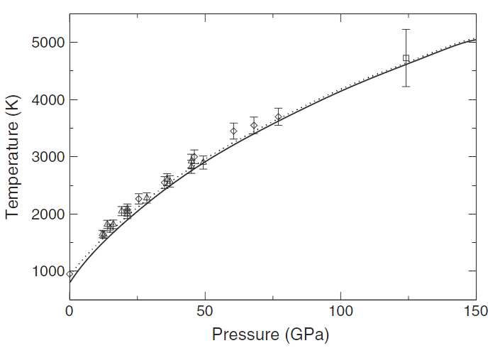
5.2 Thermite Systems ............................................................................................................. 28
      5.2.1 MoO3-Al System ......................................................................................................... 28
      5.2.2 Fe2O3-Al System ......................................................................................................... 28
   5.3 Al-O2 System ..................................................................................................................... 28
   5.4 General Observations on the Various Codes used for Calculations ................................. 30
   5.5 Thermodynamic Data Required for Future Calculations ................................................... 31
6. Incorporation of Condensed Species Equation of State in CERV ......................................... 31
   6.1 General Considerations ..................................................................................................... 31
   6.2 Addition of Physical Models .............................................................................................. 32
      6.2.1 Condensed Phase Models .......................................................................................... 32
      6.2.2 Gaseous Phase Models .............................................................................................. 33
   6.3 Improvements to Solver .................................................................................................... 33
   6.4 Expansion to Database ..................................................................................................... 34
   6.5 Summary of Requirements and Level of Importance ........................................................ 34
   6.6 Structure of CERV Code ................................................................................................... 35
7. Summary and Proposed Approach ........................................................................................ 37
8. References.............................................................................................................................. 38


                                                                                                                                            2
1.Introduction
This report discusses physical models, calculations and code capabilities for SHS detonation
modelling. The main objectives of this study are to:

    x   Summarize currently available physical models and data,
    x   Perform calculations with various equilibrium codes for selected systems,
    x   Outline CERV code capabilities and limitations,
    x   Discuss the sections of the CERV code that would be impacted by the inclusion of new
        models,
    x   Assign priorities for model development and SHS system modelling.

2.CurrentCapabilities

2.1PointsandProcesses
CERV [1] is currently capable of calculating the following thermodynamic points and processes:

    x   Thermodynamic Points
           o Temperature-Pressure (TP)
           o Temperature-Volume (TV)
           o Pressure-Volume (PV)

    x   Processes
           o Constant pressure combustion
           o Constant volume combustion
           o Detonation
           o Isentrope

A driver program has been written to perform various P-V plane calculations. The results of
these calculations are then graphically displayed through a post-processing program. The plots
generated include colour contours of various thermodynamic quantities and species
concentrations as a function of pressure and volume They also include a display of the
Rayleigh line and Hugoniot curve with constant pressure, constant volume and detonation
combustion points.

2.2PhysicalModels
CERV currently minimizes the Gibbs energy based on:

    x   NASA polynomials for the thermodynamic properties,
    x   Virial equation of state (EOS) for gases,
    x   Incompressible solids and liquids.

                                                                                             3
2.3CurrentLimitations
The main CERV code limitations include:
x Gases
o Although the third-order virial EOS, used in CERV, is suited to rocket applications
where the pressures are of the order of 0.01 GPa, it may not be accurate for
condensed explosives and SHS systems, where the detonation pressures are of
the order of 5-50 GPa.
o CERV does not currently include corrections for non-ideal mixtures.
x Condensed Species
o CERV does not include an EOS that accounts for volume change due to
compression or thermal expansion.
o Specific volumes of condensed species do not differ between the liquid and solid
phases and are often set to a default value of 2 g/cc.
o The effect of pressure on the melting temperature is not considered.
o No solution rule (ideal or non-ideal) is included. Consequently, separate melting
temperatures are assigned to co-existing condensed species. Phase diagram
topologies (eg. eutectic point) are therefore not modelled.
3.AvailableModellingApproachesforGases
3.1EquationsofState
A variety of equations of state have been proposed to model non-ideal gases. These include
classic text book models [2-4] such as :
x van der Waals
x Redlich-Kwong
x Beattie-Bridgeman
x Virial expansion
The above equations are suitable for moderate pressures and are usually based on either
empirical constants, molecular parameters and potentials, or on the law of corresponding states.
Potentials typically used for virial expansion coefficient calculations include the hard sphere,
square well, Lennard-Jones (6-12) and n-6-8 potentials [3].
The detonation of a condensed explosive generates very high pressures of the order of 20 GPa.
For such pressures, the most popular equations of state include those discussed by Davis [5].
These include:
41. Becker-Kistiakowsky-Wilson (BKW)
2. Jacobs-Cowperthwaite-Zwisler (JCZ)
3. Hayes
4. Davis
5. Williamsburg
6. JWL
7. HOM
the JWL and HOM EOS have often been used in hydrocode/CFD simulations. On the other
hand, the BKW and JCZ equations remain the EOS of choice in chemical equilibrium code
development for condensed explosives.
Various databases have been constructed for the BKW and JCZ equations of state. These
include:
x BKWC, BKWR and BKWS (Sandia)
x JCZ2, JCZ3 and JCZS (Sandia)
BKW coefficients are empirical and usually based by fitting detonation performance data. The
JCZ coefficients are more physics-based and have traditionally been obtained from
intermolecular potentials. Due to the limited available data for potential parameters, some JCZS
coefficients have also been obtained through the method of corresponding states and matching
with BKW coefficients. An excellent description of the various approaches can be found in the
Sandia report by McGee, Hobbs and Baer [6], who provide a database of JCZS parameters for
a large number of species. These authors provide many sample calculations with the JCZS
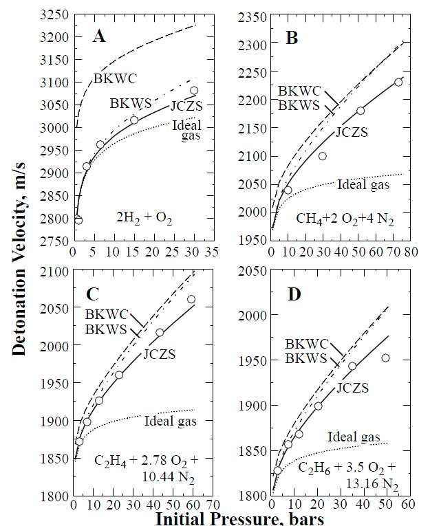
database incorporated in CHEETAH 2.0, including comparisons with experimental data for
gases and liquids. Sample comparisons are shown in Figures 1 and 2.
3.2MixtureRules
Mixtures of gaseous species are assumed 'ideal' when the total volume of the mixture may be
approximated as the sum of the partial volumes from each specie. A more realistic 'non-ideal'
mixture model takes into account the fact that the equation of state coefficients for one specie
depends on the concentrations of other species in the mixture. Various approaches to
modelling non-ideal mixtures are discussed in the book by Poling, Prausnitz and O'Connel [7],
which describes methods based on either intermolecular potentials or on the method of
corresponding states.
5Figure 1: Comparisons of experimental (circles) and computed (lines) data for
gaseous detonation velocities using different equations of state (from McGee et al
[6])
6Figure 2: Comparisons of experimental (circles) and computed (lines) data for
liquid shock pressures using different equations of state (from McGee et al [6])
74.AvailableModellingApproachesforCondensedSpecies
4.1EquationsofState
A wide variety of equations of state have been proposed for condensed solid and liquid
substances. It should be noted that various types of groups have been involved in developing
equations of state and in determining model constants based on experimental measurements
and ab initio calculations. The earth sciences community have been particularly active in this
research area, with excellent summaries provided in the books by Poirier [8] and Anderson [9].
Other areas of applications include detonics, material sciences and underwater explosions.
Recent reviews in the field of detonics may be found in the book chapters by Peiris et al [10]
and Dattelbaum et al. [11]. The most common methods to determine the EOS parameters
include:
x Diamond Anvil Cell (DAC) in conjunction with X-Ray diffraction measurements,
x Shock Hugoniot measurements,
x Detailed theoretical ab initio calculations.
Generally speaking, the EOS should address the static 'cold' compression properties, where the
temperature is maintained at a reference state, as well as the 'thermal effect' when the material
is heated to temperatures above this state. The thermal effect is closely related to the thermal
expansion properties of the substance. The total pressure, p, of a substance is therefore often
written as:
ൌ ௧
where pc is the 'cold' contribution and pth is the thermal contribution.
4.2ColdCompression
The most commonly used cold compression EOS include:
x Simple bulk modulus relation
x Birch-Murnaghan (second- and third-order) equations
x Logarithmic equation
x Vinet equation
The brief summary below is partly based on the more detailed discussion in Poirier`s book.
4.2.1SimpleBulkModulusEquation
The simplest compressibility model is based on linear elasticity where the strain is proportional
to the stress. For volumetric compression, the change in pressure may be expressed in terms
of the change in volume through the relationship:
݀ݒ ݀
ൌെ
ݒ ܭ
which may also be written as:
8݀
ܭൌെ
݀ ݒ
where K is the bulk modulus. For an isotropic solid, K may be expressed in terms of the
Young's modulus Y, and the Poisson ratio, μ, as:
ܻ
ܭൌ
ሾ͵ሺͳ െ ʹߤሻሿ
It should be noted that different definitions exist for the bulk modulus depending on the
thermodynamic variable that is held constant in the derivative of pressure. The bulk moduli KT
and Ks usually denote constant temperature and constant entropy bulk moduli respectively. The
two are related through the equation:
்ܭൌ ܭ௦ Ȁൣͳ ܸܶߙ ଶ ܭ௦ Ȁܥ ൧
where and Cp are the thermal expansion and constant pressure heat capacity respectively
[12].
4.2.2Murnaghan,TaitandSunEOS
The Murnaghan equation of state is based on the laws of elasticity and the assumption that the
bulk modulus is proportional to pressure. The pressure may then be expressed as:
ܭ ߩ ᇱ
ൌ ቈ൬ ൰ െ ͳ
ܭԢ ߩ
where the exponent, K'o , is the initial derivative of the bulk modulus with respect to pressure
and has a typical value of 3.5 for solid metals. The above equation is similar to one of the many
forms of the Tait equation of state, which is commonly used for liquids. As indicated by
Dattelbaum et al. [11] in reference to explosive binders, materials displaying many phases may
be described by the more general Sun equation of state:
ܭ ߩ ାଵ ߩ ାଵ
ൌ ቈ൬ ൰ െ൬ ൰
ሺ݊ െ ݉ሻ ߩ ߩ
which is similar in form to the Birch-Murnaghan EOS discussed below.
4.2.3BirchǦMurnaghanandLogarithmicEOS
The Birch-Murnaghan is based on the finite Eulerian strain and a power expansion of the
Helmholtz energy in terms of a parameter related to the density ratio. The second-order and
third-order expansions result in the following equations:
͵ܭ் ߩ Ȁଷ ߩ ହȀଷ
ൌ ቈ൬ ൰ െ ൬ ൰
ʹ ߩ ߩ
9͵ܭ் ߩ Ȁଷ ߩ ହȀଷ ͵ ߩ ଶȀଷ
ൌ ቈ൬ ൰ െ ൬ ൰ ቊͳ ሺܭԢ െ Ͷሻ ቈ൬ ൰ െ ͳቋ
ʹ ߩ ߩ Ͷ ߩ
with the third-order equation reducing to the second-order equation when K'o = 4. The second-
order equation can also be obtained through the selection of appropriate parameters in the
interatomic Mie potential. The Birch-Murnaghan equation may also be formulated using a
Lagrangian strain formulation. In a similar fashion, the following logarithmic equation is
obtained through an expansion involving the Henky strain:
ߩ ߩ ܭƮ െ ʹ ߩ
ൌ ܭ ͳ ൬ ൰ ൨
ߩ ߩ ʹ ߩ
4.2.4VinetEOS
Due to the power series expansions involved, the above equations lose their accuracy for very
high pressures. The following Vinet equation addresses this issue by expressing the bulk
modulus and its derivatives in terms of the interatomic distance and a scaling parameter. The
following equation is then obtained for the volume ratio.
ଷ భȀయ
ܸ ିଶȀଷ ܸ ଵȀଷ ቊ ሺᇱ ିଵሻቈଵିቀ ቁ ቋ
ൌ ͵ܭ ൬ ൰ ቈͳ െ ൬ ൰ ݁ ଶ
ܸ ܸ
Poirier presents a useful plot comparing the different equations of state for different values of Ko'
(Fig. 3). Although the results from different EOS are very similar for Ko' = 3.5, significant
differences are observed for other values.
4.3ThermalPressureandExpansion
The thermal contribution, pth, to the total pressure, p, can be described through the Mie-
Gruneisen equation:
௧ ൌ ߛ௧ ܧ௧ Ȁܸ
where Eth is the thermal energy and ߛ௧ is the thermal Gruneisen coefficient. The thermal
pressure is related to the thermal expansion which is the result of the intermolecular vibrations
and the asymmetric intermolecular potential consisting of a short-range repulsive potential and a
longer-range attractive potential. Under the quasi-harmonic assumption that the frequency
modes are independent of temperature, the thermal Gruneisen coefficient is equal to the Debye
Gruneisen coefficient, ߛ :
ߙ்ܸܭ
ߛ௧ ൌ ߛ ൌ
ܥ
where, ߙ is the thermal expansion coefficient and ܥ is the constant volume heat capacity.
Based on experimental data, Anderson [13], noted that the thermal pressure increases linearly
with temperature unless the temperature is significantly below the Debye temperature, ߠ (Fig.
4).
10Figure 3: Comparison of results for normalized pressure vs. density ratio for
different K'o using different equations of state: BME: Birch-Murnaghan (Eulerian),
BML: Birch-Murnaghan (Lagrangian), Log: Logarithmic, V: Vinet. (from Poirier [8])
Figure 4: Dependence of thermal pressure on normalized temperature (from
Poirier [8])
11As a consequence of the above linear dependence, the thermal pressure may be written as [8]:
்
߲ ் ఏವ
௧ ൌ න ൬ ൰ ݀ܶ ൌ න ߙ ܶ݀ ்ܭൌ െ න ߙ ݐ݀ ்ܭ ߙ ்ܭሺܶ െ ߠ ሻ
߲ܶ
where ߙ ்ܭis approximately constant for ܶ ߠ . As shown in Figure 5 for MgO, the thermal
expansion increases with temperature but decreases with pressure (Brosh et al. [14],
Dubrovinsky and Saxena [15]). Chang [16] has developed a scaling law, based on the Debye
temperature, that captures the temperature dependence of the thermal expansion coefficient for
various metals (Figure 6).
Figure 5: Dependence of thermal expansion coefficient on pressure and temperature
for MgO (from Brosh et al. [14], experimental data from Dubrovinski et al. [15])
Figure 6: Normalized thermal expansion coefficient as a function of the
normalized temperature for various metals (from Chang [16])
12As previously mentioned, different reference states may be used in the Mie-Gruneisen equation.
When cold isothermal compression data is available, the reference state corresponds to the
temperature at which the experiments are performed. On the other hand, if Hugoniot data are
used, the reference state corresponds to a point on the Hugoniot curve. Gheribi et al. [17] have
derived an interesting methodology relating the Hugoniot and cold compression curves for
metals. They observed that the two curves have similar shapes and can be related by
assigning a larger stiffness (or effective interatomic potential) to the material for the shock
Hugoniot. Their results indicate that the ratio of the "effective" bulk modulus for the Hugoniot
over the actual bulk modulus remains relatively constant. A similar observation is made for the
first and second derivatives of these properties. So far, the methodology has only been applied
to monatomic closely-packed metals.
Another method of including the thermal contribution in an equation of state is to allow the bulk
modulus, K, and the first derivative n = K' = dK/dp to vary with temperature. Fernandez [18] has
applied this method to the Murnaghan equation of state. The temperature dependence is
calculated based on a Gruneisen coefficient for a Debye solid. The temperature dependence of
n can be expressed as a second-order polynomial.
Many of the thermal pressure models described above are based on a Gruneisen coefficient
which varies with volume. If the thermal Gruneisen coefficient, ߛ௧ , is used, the variation of this
ఊ
coefficient can be quite reasonably approximated by assuming that the ratio is constant. It
should be noted that a variety of Gruneisen coefficients are used in the modelling of material
properties. Some of these are based on material properties at the atomic level, while others are
based on more macroscopic properties and measurements. A good description of the various
Gruneisen coefficients is presented in Poirier's book. As noted by Vocadlo et al. [19], there
exist significant differences between the various Gruneisen coefficients and those calculated
from detailed ab initio calculations. A judicious choice of a suitable Gruneisen coefficient must
be made when applying it to a particular equation of state or Hugoniot. This point has also been
emphasized by Segletes [20].
4.4MeltingofMetals
4.4.1MeltingParameters
Melting of a material is associated with the loss of resistance to shear and long-range crystalline
order. Some important parameters associated with melting include:
x The melting temperature Tm, which depends on the pressure,
x The change in volume οܸ ൌ ܸ െ ܸௌ between the liquid and solid state,
x The change in entropy οܵ ൌ ܵ െ ܵௌ between the liquid and solid state,
x The latent heat of melting ܮ ൌ ܶ οܵ .
4.4.2ClausiusǦClapeyronEquation
The simplest equation relating the above parameters is that of Clausius-Clapeyron:
݀ܶ οܸ
ൌ
݀ οܵ
13Knowing the melting temperature, the volume change and the latent heat of melting, the above
equation may be used to obtain the initial linear dependence of the melting temperature with
pressure near atmospheric pressure.
4.4.3EquationsBasedonLindemannLaw
As seen from Figure 7 [21], the linear Clausius-Clapeyron relationship is no longer valid for
higher pressures, with the non-linearity being more pronounced for softer materials. The most
popular models to predict this nonlinear dependence are based on the law of Lindemann [22].
Poirier presents an excellent description of this law with the extension developed by Gilvarry
[23]. Further modifications to these models have also been presented by Schossler et al. [21]
and Fang et al. [24].
The original Lindemann-Gilvarry model is based on the notion that the melting point is based on
a critical level of atomic vibrations relative to the interatomic distance rm. Following the
discussion by Poirier [8], the melting criteria is then presented as:
ݑۃଶ ۄൌ ݂ ଶ ݎଶ
where ݑۃଶ ۄis the mean-square atomic velocity and ݂ is an empirical constant that is
approximately 0.08 for metals. For high temperatures and a monoatomic solid, ݑۃଶ ۄmay be
estimated as:
ͻ݄ଶ ܶ
ݑۃଶ ۄൌ
݉݇ ߠଶ
where, m is the atomic mass, D is the Debye temperature and h and kB are the Planck and
Boltzmann constants respectively. The melting temperature is then given as:
݇
ܶ ൌ ݂ ଶ ݉ߠଶ ݎଶ
ͻ݄ଶ
Lennard-Jones and Devonshire [25] have provided a theoretical justification of the empirical
Lindemann-Gilvarry model based on the Lennard-Jones potential. Since rm varies with pressure
and is related to the specific volume, the Lindemann law is usually used in conjunction with an
equation of state to determine the pressure dependence of the melting temperature.
As can be seen from the calculations of Schossler et al. [21] (Figure 7) and Fang et al [24],
predictions based on the Lindemann-Gilvarry approach provide good agreement for
monoatomic metals. As indicated by Poirier, however, the predictive capability of the models
are significantly lower for more complex molecules. As will be discussed below, some of these
limitations have been addressed in the more recent work of Shen et al. [26-27] and Wang et al.
[28-29] and by more detailed and fundamental ab initio calculations.
14Figure 7: Dependence of melting temperature on pressure. Solid
lines represent model predictions, (from Schlosser et al. [21]).
15 4.4.4ModelsbasedonVolumeChange
Useful relationships have been derived between the entropy and volume changes οܵ and οܸ
for melting. Oriani [31] and Tallon [32] proposed the relationship:
οܵ ൌ ܴ݈݊ʹ ߙ ்ܭοܸ
The first and second terms are the configurational and thermal entropy respectively. Since ߙ்ܭ
is approximately constant, the above relationship implies that the entropy change is proportional
to the volume change. The entropy change can be expressed in terms of the melting
temperature and the latent heat of melting. The entropy change associated with melting has
been estimated by Wallace [32] for 25 elements.
4.4.5Wang,LazorandSaxenaModel
As previously indicated, the Lindemann-Gilvarry model has been applied most successfully to
monoatomic metals for pressures below 10GPa. Wang et al. [29] have developed a simple
thermodynamic model that has been applied to polyatomic molecules for pressures as high as
100 GPa. The model is based on calculating the 'critical' melting temperature, which is related
to a critical volume. The procedure relates the pressure-dependent melting temperature to
thermodynamic properties at ambient pressure. These include the isothermal bulk modulus and
the solid molar volume at room temperature, the isothermal bulk modulus and liquid molar
volume at the melting point, the bulk modulus derivative, and the average product of the thermal
expansion and the bulk modulus. The analysis is based on the Birch Murnaghan EOS and a
thermal pressure which, as previously discussed, is related to the product of the thermal
expansion coefficient, the isothermal bulk modulus and temperature differential. Computations
and comparisons with experiments have been performed for lithium fluoride (LiF), diopside
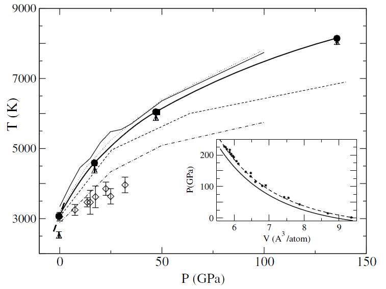
(CaMgSi2O6) and wustite (FeO). As seen from Figure 8 for LiF, the model calculations compare
very well with experimental data for pressures as high 95 GPa. The model is also significantly
more accurate than the Lindemann model at higher pressures. It can also be seen from Figure
9 that the model provides data for the thermal pressure and the melting molar volume as a
function of pressure. This type of data is of particular relevance to assessing the SHS
detonation potential of a system.
4.5ExperimentalDataandAbInitioCalculations
The data required for the various EOS parameters and melting properties models may be
obtained from experimental data or ab initio calculations based on fundamental intermolecular
potentials and quantum statistical mechanics. High pressure experimental data are usually
obtained from Diamond Anvil Cell (DAC) or shock Hugoniot measurements. Ab initio
calculations are based on molecular dynamics calculations using the Density Functional Theory
(DFT). A description of the DFT methodology can be found in computational chemistry text
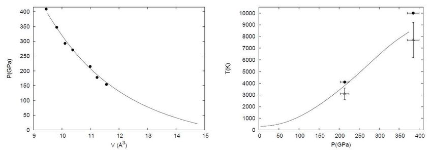
books such as that by Cramer [34]. Figure 10, from Cazorla et al. [35], displays comparisons
between experimental and theoretical data for the shock Hugoniot and melting temperature of
molybdenum. Figures 11 and 12, from Alfe et al. [36,37], display similar comparisons for Al and
MgO. An overview of ab initio modelling capabilities for the calculation of melting properties can
be found in the article by Alfe et al. [36].
16Figure 8: Melting temperature predictions using Wang et al. and
Lindemann models, and experimental data for LiF system [29].
Figure 9: Melting thermal pressure and molar volume predictions
using Wang et al. model for LiF system [29].
17Figure 10: Comparisons of experimental and ab initio data for the Hugoniot and
melting temperature of molybdenum, from Carzola et al. [35]
Figure 11: Comparisons of experimental and ab initio data for the melting
temperature of Aluminium, from Alphe et al. [36]. Solid and dotted lines are ab
initio results. Diamonds and square denote the experimental DAC and Hugoniot
data.
184.6SolutionRules
Figure 12: Comparisons of experimental and ab initio data for the Hugoniot and
melting temperature of MgO, Alphe [37]. Solid squares, rectangles and solid
lines represent ab initio calculations using 432 and 1024-atom cells. Triangles
represent DFT-CGA calculations and open diamonds denote the experimental
data.
The above discussions have focused on properties of single-component systems. Mixture or
'solution' rules are required to model multi-component systems. For solids and liquids, the
solution rules may be classified into three categories:
x Ideal solution
x Regular solution
x Non-regular solution
With the exception of CALPHAD-based codes, equilibrium codes do not usually include any
solution rules in their calculations. This implies that each component has its own melting
temperature and is not affected by the presence of any other component. Due to the
development of CALPHAD codes, which began in the 1970's, considerable work has been done
on the formulation of solution rules for different types of solid crystal structures. Comprehensive
descriptions of this work may be found in the books by Saunders and Miodownik [38] and by
Hillert [39].
194.6.1GibbsEnergyofMixing
Solution rules are introduced into an equilibrium calculation through the addition of a mixing
energy to the overall Gibbs energy to be minimized. For a system containing species A and B,
the total Gibbs energy is then given by:
்ܩ௧ ൌ ݔ ܩ ݔ ܩ ܩ௫
where ܩ௫ is the Gibbs energy of mixing.
IdealSolution
An ideal solution simply accounts for the increase in configurational entropy during mixing and
assumes no attractive or repulsive forces between the atoms of the two different components, A
and B. In this case, the Gibbs energy of mixing is given by:
ܩ௫
ௗ
ൌ ܴܶሺݔ ݈݊ݔ ݔ ݈݊ݔ ሻ
It can be seen from the above equation that an ideal solution model does not require any
additional thermodynamic data beyond that for the individual components, A and B.
RegularandNonǦRegularSolution
When the attraction and repulsion between components are considered, an additional 'excess
energy' , ܩ௫
௫௦
is introduced and added to the ideal solution contribution. In this case,
ܩ௫ ൌ ܩ௫
ௗ
ܩ௫
௫௦
For a regular solution, the excess energy is given by:
ܩ௫
௫௦
ൌ ݔ ݔ ȳ
where is positive or negative for repulsive or attractive potentials respectively. Different
values of must be obtained for liquid and solid solutions to construct a phase diagram. As
illustrated in Figure 13 from Pelton [40], the sign and magnitude of these values play an
important role in determining the topology of the phase diagram. For non-regular solutions,
additional terms are added to the ideal solution mixing energy using a power series of
interaction terms. The temperature-concentration (T-C) diagrams are also dependent on the
system pressure. Figures 14 and 15 display computed and experimental phase diagrams for
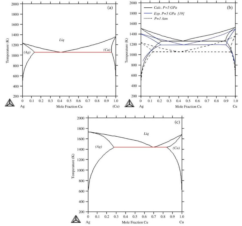
Al-Si (Brosh et al. [14]) and Ag-Cu (Gheribi et al. [41]) at ambient and elevated pressures.
20Figure 13: Different phase diagram topologies as a function of
liquid and solid excess energy [40]
5.EquilibriumCalculationsforSHSSystemsofInterest
Several systems have been proposed for SHS combustion [42]. The purpose of this section is
to present some sample equilibrium calculations using various equilibrium codes. These
include CERV [1], FactSage [43], CEA [44] and Thermo [42,45]. Systems such as Ti-Si and Ti-
B are not only energetic but remain essentially gasless during combustion even at ambient
atmospheric pressure. 'Thermite' reactions involving F2O3-Al or MoO3-Al can generate
significant amounts of gaseous products when burned at 1 atm. However, such systems may
indeed be gasless at detonation pressures. Thermite systems offer the advantage that the
reactants and products have been extensively studied at high pressure. The discussion below
presents phase diagrams and equilibrium constant pressure combustion calculations for these
two types of systems.
5.1TiǦSiandTiǦBSystem
5.1.1TiǦSiSystem
Figure 16 presents Ti-Si phase diagrams from Massalski [46] and calculated using FactSage.
The results are similar with the exception that FactSage combines the Ti5Si3 and Ti5Si4 regions
into a solid solution of the two combustion products. It should also be noted that FactSage
calculations use a liquid phase database that only contained the reactants Ti and Si. As
21indicated in Figure 17, FactSage can also compute the gas phases at higher temperatures.
FactSage was used to calculate the constant pressure combustion temperature as a function of
concentration. The results are included with the phase diagram in Figure 18. Also shown, are
results computed using the Thermo equilibrium code [42]. The main difference between the two
calculations is that Thermo contains the liquid phase products TiSi and Ti5Si3, which are not
available in the FactSage database. FactSage calculations indicate a maximum temperature for
a stoichiometric composition for the reaction 3Ti + 5Si -> Ti3Si5. Finally, no results from CERV
or CEA are displayed in the figure since the databases used by these codes to not contain any
of the required combustion products in solid or liquid phases.
5.1.2TiǦBSystem
The results of similar calculations are provided below for the Ti-B system. As seen from Fig. 19,
the FactSage phase diagram differs from that from Massalski in the central region of the
diagram due to a 'B2M' prototype solution model used in that region. Figure 20 displays the gas
regimes that occur at higher temperatures. Constant pressure combustion temperatures are
displayed in Fig. 21 based on calculations performed using FactSage, Thermo and CERV. The
calculations using FactSage and Thermo are more consistent than for the Ti-Si system since
the databases used by both codes contain the dominant combustion products TiB (solid),
TiB2(solid) and TiB2(liquid). One important difference between the two calculations is that
Thermo predicts a peak temperature for the (1Ti + 1B) system (boron mole fraction, 0.5),
whereas FactSage indicates a peak temperature for the (1Ti + 2B) system (boron mole fraction,
0.667). CERV and CEA use a similar database that also contain the desired phases of the TiB
and TiB2 combustion products. However, CERV only converged for two points yielding
significantly lower temperatures than FactSage and Thermo. Finally, CEA calculations did not
converge for this system. This may be due to the fact that the combustion for this system is
gasless. It is possible that better convergence could have been obtained by arbitrarily adding a
small mole fraction of inert gas in the reactants.
22Figure 14: Phase diagrams for Al-Si system at different pressures [14]
Figure 15: Phase diagrams for Ag-Cu system at different pressures
[41]. a) standard pressure, b) 5 GPa and c) 10 GPa.
23Figure 16: Phase diagrams for Ti-Si system: Massalski [46] (top),
FactSage (bottom).
24Gas
Liquid
Figure 17: Phase diagrams for Ti-Si system showing gas phase at
higher temperatures (computed using FactSage).
Liquid
Liquid +
Ti5Si3(S)
Liquid +
Ti5Si4(S)
Liquid +
TiSi(S)
Liquid + Ti5Si3(S)
Liquid +
Si(S)
Liquid +
BCC_A2 + Ti5Si3(S) TiSi(S) + TiSi2(S) TiSi2(S) + Si(S)
T TiSi2(S)
Ti5Si4(S) +
TiSi(S)
HCP_A3 + Ti3Si(S)
Ti5Si3(S) +
Ti5Si4(S)
Figure 18: Comparison of constant pressure combustion temperatures
using FactSage (+) and Thermo (o) [42].
25Figure 19: Phase diagrams for Ti-B system: Massalski [46] (top),
FactSage (bottom).
26Gas
Liquid
Figure 20: Phase diagrams for Ti-B system showing gas phase at
higher temperatures (computed using FactSage).
Liquid + B2M
Liquid
Liquid + B2M
Liquid +
TiB2(L)
Liquid + TiB(S)
B2M + TiB(S)
B2M
B2M + B(S)
BCC_A2 + TiB(S)
TiB(S) + Ti(S)
Figure 21: Comparison of FactSage (+), Thermo [42] (o) and CERV (*)
constant pressure combustion temperatures for Ti-B system.
275.2ThermiteSystems
5.2.1MoO3ǦAlSystem
Constant pressure combustion properties for the MoO3-Al system were calculated using
FactSage, CERV and CEA. The results are included in a phase diagram computed using
FactSage (Fig 22). The FactSage calculations indicate that the combustion temperature peaks
for a stoichiometric mixture corresponding to the reaction MoO3 + 2 Al -> Mo + Al2O3. The
results from the CERV calculations are very different and suggest a strongly exothermic
decomposition combustion for pure MoO3, which is not observed in the FactSage calculations.
This is due to the fact that the CERV database does not include the required solid phase of
MoO3 in its thermodynamic database. FactFage calculations indicate that, for temperatures
below 1060oC, significant concentrations of condensed MoO3 remain in the products for Al
mole fractions lower than 0.4. CEA had considerable difficulty converging to results unless
specific condensed species were omitted or included based on the FactSage calculations.
When this was done, CEA provided similar results as FactSage for the cases where CEA
converged. A similar comparison was not possible with CERV since the code does not currently
provide the option to include or omit specific species or phases from the calculations. Finally,
no Thermo results have been reported for thermite systems in ref [42].
5.2.2Fe2O3ǦAlSystem
Figure 23 provides comparisons between FactSage and CERV calculations for the Fe2O3-Al
system with results that are qualitatively very similar to those for the MoO3-Al system. The
Fe2O3-Al system results in lower combustion temperatures with CERV once again predicting
high combustion temperatures for pure Fe2O3 due to the lack of thermodynamic data for the
condensed phases of this oxide. It can be noted that the phase diagram computed by FactSage
is not totally complete. It is not clear at this time whether this is a computational or graphical
problem.
5.3AlǦO2System
Due to the discrepancies observed above for thermite systems, calculations were performed for
the simple Al-O2 system to determine if the various code/database combinations computed
different results for aluminium oxidation. Figure 24 displays constant pressure combustion
temperatures computed with FactSage, CERV and CEA. As in previous cases, the phase
diagram was calculated using FactSage. CERV calculations did not converge for very low or
high concentrations of O2 due to the fact that the code encounters convergence problems at
temperatures below approximately 500 oC. With the exception of one point, where the CERV
value is slightly higher, the results obtained from the three codes are very similar. This would
indicate that the main differences observed for the thermite system are related to reactions that
involve Mo or Fe.
28Gas
Gas + Liquid
Gas + Al2O3 (L)
Gas + Al2O3 (L) + Mo(L) Gas + Liquid +
Al2O3 (L)
Gas + Al2O3 (L) + Mo(S)
Liquid + Al2O3 (L)
Mo(S) + Al2O3 (S)
Gas + Al2O3 (S) + MoO2(S) + MoO2(S)
Al2O3 (S) + MoO2(S) + MoO3(L)
Al2O3 (S) + MoO2(S) + MoO3(S)
Figure 22: Comparison of FactSage (+) , CERV (o) and CEA (*)
calculations for the constant pressure combustion temperatures for the
MoO3-Al system.
Gas
Gas + Al2O3 (L)
Gas + Liquid +
Al2O3 (L)
Gas + Al2O3 (L)
+ FeO(L)
Liquid + Al2O3 (L)
+ FeO(L)
Liquid + Al2O3 (L)
FeO (L) +
FeAl2O4(S) +
FeO (S) + Fe(L)
FeAl2O4(S) +
Fe3O4(S)
Al2O3 (S) +
Fe3O4(S)+
Fe2O3(S)
Figure 23: Comparison of FactSage (+) and CERV (o) calculations for
the constant pressure combustion temperatures for the Fe2O3-Al
system.
29Gas
Liquid +
Gas
Gas + Al2O3 (L) Gas + Al2O3 (L)
Liquid +
Al2O3 (L)
Liquid + Al2O3 (S) Gas + Al2O3 (S)
Figure 24: Comparison of FactSage (+) and CERV () and CEA (*)
constant pressure combustion temperatures for the Al-O2 system.
5.4GeneralObservationsontheVariousCodesusedforCalculations
Comparisons between different equilibrium codes remain difficult due to the fact that they
typically use not only different solvers, but also different databases for the thermodynamic
properties. In spite of this, the calculations presented above do shed some light on the overall
robustness of the code.
The CALPHAD-based FactSage code solver seems to be very robust as no convergence
problems were encountered during the equilibrium calculations performed in this study. Such
solver performance is probably not surprising since CALPHAD codes are expected to calculate
complex phase diagrams. This requires good convergence capabilities for a wide range of
component concentrations and thermodynamic states. FactSage does not have a complete
database for the condensed phase combustion products. In particular, limited data is available
for the molar volumes, which are of particular importance in assessing SHS detonation
feasibility. The code also does not currently support calculations for detonation or for constant
volume combustion, where both the volume and internal energy is kept constant. It is possible
that such capabilities could be implemented through the ChemApp software library [47], which
provides a C or FORTRAN interface to the chemical equilibrium solver and database.
Although CERV and CEA use a very similar database, CERV appears to offer superior
convergence performance, except for calculations involving low temperatures below 500 oC.
Both CERV and CEA had difficulties with calculations involving the Ti-B system and did not
30have the required condensed phase combustion products in their database to compute the Ti-Si
system. Although CEA has been used successfully for a wide range of gaseous systems, it
often encounters matrix singularities and fails to converge for systems involving condensed
species. When convergence is actually achieved, the user is often required to insert or omit
selected species. This procedure is not only tedious but can require some prior knowledge of
the solution, which diminishes the code's predictive capabilities.
Very little is known concerning the solver and database used by the Thermo code. Based on
the results presented in reference [42], the code seems to include thermodynamic data for a
wide range of gaseous and condensed species. Since final system densities are not reported in
this reference, Thermo may also lack the molar volume data required for such a calculation. As
with FactSage, Thermo does not support detonation calculations.
5.5ThermodynamicDataRequiredforFutureCalculations
The eventual computation of detonation properties for SHS systems will require suitable data for
the:
1. Thermodynamic properties and molar volume for the relevant phases,
2. Equation of state parameters,
3. Melting temperature dependence on pressure.
As previously stated, the pressure range of interest for SHS detonation is of the order of 5-50
GPa, depending on the mixture components and the system porosity. Some of this data is
available for monatomic metal elements and for minerals of particular interest to geophysics. As
can be seen from references 48-64, numerous experimental and numerical studies have been
performed for materials relevant to the systems discussed in this report. Most of the available
data, however, are mainly relevant to thermite systems due to the relevance of the reactants
and combustion products to earth sciences. These experimental data are obtained through the
combined use of a Diamond Anvil Cell (DAC) and X-Ray diffraction. The most promising
theoretical work has been performed using ab initio calculations based on the Density
Functional Theory (DFT). Key laboratories for these studies include the earth science groups at
the Uppsala University (Sweden) for the experimental work, and the University College London
(UK) for numerical studies. In addition to the listed publications in the reference section of this
report, these institutions represent a potentially good source of information concerning available
data for some of the SHS systems of interest. The first priority should focus on obtaining the
data required to determine the volume expansion after constant pressure combustion. This is
important since a positive volume expansion is required for SHS detonation.
6.IncorporationofCondensedSpeciesEquationofStateinCERV
6.1GeneralConsiderations
As noted in Section 2 of this report, CERV can now model a variety of thermodynamic states
and processes, with post-processing capabilities to construct plots in the P-V plane. This has
been possible through the following activities:
311. Re-structuring of the code by UTIAS to provide a library of subroutines for a variety of
problem types (TP, TV, HP and UV),
2. The use of the above routines by TimeScales Scientific Ltd. to construct new
subroutines for additional problem types (PV, isentrope, sound speed, Hugoniot and
detonation),
3. The development by TimeScales of a post processor program to create the required
plots in the P-V plane.
Section 2.3 of this report summarizes some of the current CERV limitations. The purpose of
this section is to discuss these limitations in greater detail, with the aim of prioritizing future code
development activities, which include:
1. Addition of physical models,
2. Improvements to the code solver to enhance convergence characteristics,
3. Expansion of the database.
6.2AdditionofPhysicalModels
The modelling of SHS detonations will require model improvements for condensed and gaseous
phases. Since one of the main objective of the SHS detonation research is to achieve gasless
combustion, the condensed phase models are of greater importance and will be discussed first.
6.2.1CondensedPhaseModels
The main requirements for improvements to the condensed phase calculations in CERV include
models for:
1. Compressibility,
2. Thermal expansion,
3. Dependence of melting temperature on pressure,
4. Solid and liquid phase molar volumes,
5. Solution modelling.
As discussed in Sections 4.2 and 4.3 of this report, the first two requirements involve the
inclusion of an equation of state that can accommodate "cold " isothermal compression along
with thermal expansion. Various models have been developed for isothermal compression
ranging from a simple bulk modulus model to more detailed Birch-Murnaghan, logarithmic and
Vinet models that involve additional parameters such as the pressure derivative of the bulk
modulus. The thermal expansion is introduced through a Mie-Gruneisen equation where a
suitable Gruneisen coefficient must be chosen. This report provides various thermodynamic
relations and approximations that facilitate the estimate of some of the relevant parameters.
Assuming that more complex equations of state do not introduce any specific convergence
problems, the introduction of increasingly more accurate models should not pose any major
difficulties. One consideration is that CERV currently uses state variable derivatives for its
minimization of the Gibbs energy. If the condensed species EOS are not easily differentiated,
32suitable differentiable curve fits to the EOS could be developed. Alternatively, a lower order
minimization process, not requiring derivatives, could be used.
The successful modeling of SHS detonations requires the ability to incorporate different molar
volumes for solid and condensed phases, along with the accommodation of a melting
temperature that is dependent on pressure. Whereas the first requirement depends of the
availability of suitable experimental or ab initio calculation data, the second requirement can be
accommodated through one of many available melting models. The theory of Lindemann and
Gilvarry theory has been particularly successful in modeling monatomic metals. Although the
modelling of polyatomic combustion products is more challenging, promising results have been
obtained for such systems using the more recent model by Wang et al [29] and by applying
more fundamental ab initio methods.
An accurate modelling of a SHS mixture through a range of compositions requires the
introduction of solution models of the type commonly used in CALPHAD codes. Due to the level
of effort involved, it would not be realistic to introduce full solution modelling capabilities in
CERV. Nevertheless, an ideal solution model could be introduced relatively easily based on the
discussion in Section 4.6 in this report. Limited non-ideal solution modelling capabilities could
possibly be introduced for a very specific region of the phase diagram by fitting solid and liquid
excess energies to obtain results that are consistent with phase diagram data obtained from
experiments or from separate CALPHAD code calculations.
6.2.2GaseousPhaseModels
As previously noted, CERV currently uses a virial expansion, which is probably not suited for the
very high pressures generated by SHS detonations. JCZ equations of state, initially developed
for condensed explosives, would be more suitable to accommodate such pressures. This
limitation may not be serious if the SHS combustion is gasless at atmospheric pressure, or
becomes gasless at the elevated detonation pressure. In the latter case, the gases would only
be produced when the combustion products have been expanded to a lower pressure where
gases are eventually produced. For most systems of interest, the pressure where this occurs
may be low enough for the virial expansion to remain valid. In this case, the only requirement
for the EOS is to be reasonably well behaved at very high pressures to prevent solver
convergence failure and avoid the calculation of a totally incorrect state. Finally, CERV
currently assumes an ideal gaseous mixture and therefore neglects the cross-terms for the virial
EOS coefficients. Once again, considering that the main interest is in gasless combustion, this
limitation may not be very significant.
6.3ImprovementstoSolver
As previously noted, CERV does not currently provide the same level of convergence
robustness as CALPHAD-based codes such as FactSage. CERV also encounters convergence
difficulties at lower temperatures. This not only causes problems for systems with relatively low
exothermicity, but prevents calculations of the 'frozen' Hugoniot for the unreacted material. The
code also encounters difficulties for some systems such as, Ti-B, where converged results are
only obtained for a narrow range of concentrations. The underlying reasons for these
convergence problems need to be identified to allow suitable remedies to be implemented.
336.4ExpansiontoDatabase
CERV is currently based on a NASA database that is similar to that used by CEA. This
database has been developed for gases and incompressible condensed phases. As indicated
in the calculations performed for this report, the database lacks the appropriate condensed
phase combustion products to model the Ti-Si system or the Fe2O3 and MoO3 reactants for
thermite systems. Although the database provides an entry field for the liquid and solid phase
densities, the actual data for the values are lacking for the systems of interest. Finally, an
additional database is required to store equation of state parameters for the condensed phases
as well as the pressure dependence of the melting temperature. One important factor to keep in
mind is the requirement that new models and data must be introduced into the equilibrium code
in a way that ensures that the overall thermodynamic data is self consistent. Finally, in order to
allow comparisons with other codes and databases, CERV should allow the user the option to
add and remove selected species and phases.
6.5SummaryofRequirementsandLevelofImportance
Requirements Level of ID
Importance
Physical Models
Condensed Phase
Compressibility A P1
Thermal expansion A P2
Melting temperature as a function of pressure A P3
Solid and liquid phase molar volume A P4
Solution modelling (ideal and non-ideal) C P5
Gas Phase
JCZ equation of state C P6
Non-ideal mixture D P7
Database Expansion
Thermo data for condensed phases of all reactants and products A D1
Compressibility and thermal expansion data A D2
Melting temperature and molar volumes A D3
Solution excess energy parameters C D4
Allow insertion and removal of specie/phase B D5
Solver Capabilities
Improve convergence for low temperature B S1
Improve convergence for range of SHS systems A S2
Improve solver speed D S3
Consolidate Gibbs energy minimization into a separate function B S4
34Based on the above discussions, the table above summarizes the overall CERV development
requirements and assigns a level of importance from A to D, with A being the most important.
The table also includes some requirements that are specific to the equilibrium solver such as
improving the convergence and speed, and separating sections of the code that are repeated in
the various subroutines. These code sections could be consolidated into separate subroutines.
Sections that could be consolidated include those used for Gibbs energy minimization and root
solving.
6.6StructureofCERVCode
The current CERV code is based on a library of subroutines that are used for different types of
problems. The main subroutines, where equilibrium concentrations are calculated, correspond
to those associated with the TP, TV, UV and HP problems. These subroutines access the
database and minimize the Gibbs energy. The additional subroutines developed by TimeScales
use these subroutines rather than directly call the equilibrium solver. The latter subroutines will
therefore not be greatly impacted by changes in the database or the equilibrium solver. The
overall structure of the equilibrium code is displayed below for the subroutine responsible for TP
calculations.
Subroutine tp_problem
x scalnatm: scale the number of atoms
x select: select product species
o inisiep: initialize collision diameters and attraction potentials
step:s estimate and initialize collision diameters and attraction potentials
x wmconv: convert weight percentages of reactants to mole percentages
o ludcmp
o lubksb
x transtemp: calculate transition temperatures for condensed species pairs
o dmu0
x du: calculate the difference in internal energy of reactants and products
o sort: sort array in descending order
o stoichi :matrix reduction
o ortho: determine independence among a set of vectors
o vir_coe: calculate virial coefficients for ideal mixture
o con : calculate equilibrium composition using the modified virial equation of state
chmpot: calculate chemical potentials of gaseous species (ideal mixture)
x pres: calculate pressure
o dv : calculate gaseous and condensed species volumes
kalpa: determine step size for positive mole numbers
lambda: determine step size to find minimum Gibbs energy
x chmpot: calculate chemical potentials of gaseous species only
x melt: calculate equilibrium composition at transition temperature
o ortho: determine independence among a set of vectors
o stoichi :matrix reduction
o intlx: calculate initial mole numbers of gaseous and condensed species (minimize
Gibbs energy)
gg: calculate Gibbs energy
simplx: simplex method
stoichi :matrix reduction
o gg: calculate Gibbs energy
o sort: sort array in descending order
35You can also read