Absolute instability in shock-containing jets
←
→
Page content transcription
If your browser does not render page correctly, please read the page content below
This draft was prepared using the LaTeX style file belonging to the Journal of Fluid Mechanics   1

                                                    Absolute instability in shock-containing jets
arXiv:2106.12690v1 [physics.flu-dyn] 23 Jun 2021

                                                   Petrônio A. S. Nogueira1 †, Peter Jordan2 , Vincent Jaunet2 , André V.
                                                      G. Cavalieri3 , Aaron Towne4 , and Daniel Edgington-Mitchell 1
                                                   1
                                                     Department of Mechanical and Aerospace Engineering, Laboratory for Turbulence Research
                                                                  in Aerospace and Combustion, Monash University, Clayton, Australia
                                                        2
                                                          Département Fluides, Thermique, Combustion, Institut PPrime, CNRS–Université de
                                                                                   Poitiers–ENSMA, Poitiers, France
                                                      3
                                                        Divisão de Engenharia Aeronáutica, Instituto Tecnológico de Aeronáutica, São José dos
                                                                                    Campos, SP, 12228-900, Brazil
                                                    4
                                                      Department of Mechanical Engineering, University of Michigan, 2350 Hayward Street, Ann
                                                                                         Arbor, MI 48109, USA
                                                                                 (Received xx; revised xx; accepted xx)

                                                   We present an analysis of the linear stability characteristics of shock-containing jets.
                                                   The flow is linearised around a spatially periodic mean, which acts as a surrogate for a
                                                   mean flow with a shock-cell structure, leading to a set of partial differential equations
                                                   with periodic coefficients in space. Disturbances are written using the Floquet ansatz
                                                   and Fourier modes in the streamwise direction, leading to an eigenvalue problem for the
                                                   Floquet exponent. The characteristics of the solution are directly compared to the locally
                                                   parallel case, and some of the features are similar. The inclusion of periodicity induces
                                                   minor changes in the growth rate and phase velocity of the relevant modes for small
                                                   shock amplitudes. On the other hand, the eigenfunctions are now subject to modulation
                                                   related to the periodicity of the flow. Analysis of the spatio-temporal growth rates led to
                                                   the identification of a saddle point between the Kelvin-Helmholtz mode and the guided
                                                   jet mode, characterising an absolute instability mechanism. Frequencies and mode shapes
                                                   related to the saddle points for two conditions (associated with axisymmetric and helical
                                                   modes) are compared with screech frequencies and the most energetic coherent structures
                                                   of screeching jets, resulting in a good agreement for both. The analysis shows that a
                                                   periodic shock-cell structure has an impulse response that grows upstream, leading to
                                                   oscillator behaviour. The results suggest that screech can occur in the absence of a nozzle,
                                                   and that the upstream reflection condition is not essential for screech frequency selection.
                                                   Connections to previous models are also discussed.

                                                   Key words: Authors should not enter keywords on the manuscript.

                                                   1. Introduction
                                                     With the development of commercial and military aviation in the last century, the
                                                   importance of studies on noise generation by jets has increased substantially. These
                                                   studies can be divided into two broad categories, based on the source mechanisms
                                                   responsible for noise generation. The first category is shock-free jets, comprising both
                                                   subsonic jets and ideally-expanded supersonic jets; the acoustic field of such flows is
                                                   usually dominated by the noise generated by organised structures present in the turbulent
                                                                 † Email address for correspondence: petronio.nogueira@monash.edu
2                                P. A. S. Nogueira et al.
flow (Jordan & Colonius 2013), which underpin both Mach wave radiation (for supersonic
jets), and turbulent mixing noise (subsonic and supersonic cases). The second category
is shock-containing jets, i.e., imperfectly expanded supersonic jets. In this case, the
pressure deficit between the choked nozzle and external medium leads to the appearance
of a spatially periodic coherent structure formed by several shock-cells (Pack 1950).
The appearance of shock cells dramatically impacts the acoustics of these jets, with
the appearance of two other components due to the interaction between the organised
structures and the shocks (Tam 1995): broadband shock-associated noise (BBSAN),
usually peaking at slightly higher frequencies than the turbulent mixing noise, and screech
tones, associated with high intensity pressure fluctuations at specific frequencies.
   The earliest description of the screech phenomenon was that of Powell (1953a). Using
schlieren photographs, Powell identified the presence of large-scale turbulent structures
travelling downstream and acoustic waves travelling upstream in shock-containing jets.
Motivated by these observations, he proposed that screech tones are generated by a self-
sustained resonant process involving both waves, where the interaction between the large-
scale structures and the shocks gives rise to acoustic waves that excite new downstream-
travelling structures upon reaching the nozzle lip. As usual in the analysis of resonant
phenomena, both phase and gain conditions for this process were derived (Powell 1953b)
and applied to the study of screeching jets. Powell’s theory managed to predict screech
tones and directivities with relative success, being used as the foundation of several
subsequent analyses, as summarised by Raman (1998) and Edgington-Mitchell (2019).
   While the downstream propagation of energy is quite well understood, the process of
upstream wave generation in this cycle is still under investigation. While the original
work of Powell (1953a) proposes a multiple, discrete-source formulation, related to the
position of each shock-cell, other works have proposed alternative views. For instance,
Tam & Tanna (1982) proposed a formulation based on a frequency-wavenumber analysis
of the different waves in the jet, leading to a continuous source distribution in the
turbulent medium. In this previous work (also in Tam et al. (1986)), the authors propose
that screech is a direct consequence of the interaction between shock-cell and large-
scale structures in the wavenumber domain. In this framework, no position for the
generation of upstream waves is imposed, and predictions are performed by analysing
the wavenumbers energised by such interaction. More recently, Gojon et al. (2018) and
Edgington-Mitchell et al. (2018) have shown that the resonance mechanism may actually
be closed by a neutrally stable guided jet mode, as opposed to an acoustic wave. This
mode has specific bands of existence that roughly match the regions where screech tones
are found experimentally. Resonance models using these guided jet modes lead to a better
alignment with experimental data, strongly supporting this hypothesis (Mancinelli et al.
2019, 2020; Nogueira et al. 2020). The work of Manning & Lele (1998, 2000) proposed
a mechanism for generating upstream waves, in which the complex interaction between
vortices and shocks would give rise to acoustic waves. The model managed to reproduce
characteristics of screech observed in experiments (Shariff & Manning 2013; Edgington-
Mitchell et al. 2021b), even with strong simplifications of its underlying assumptions.
   While early models for the analysis of jet turbulence, including screech, were based
on experimental observations and classic resonance theory, the development of stability
theory helped to uncover the physics of the problem. Tools based on this theory have been
used extensively in the analysis of flow dynamics and sound generation in subsonic jets
(Michalke 1964, 1965; Crow & Champagne 1971; Michalke 1971; Crighton 1975; Cavalieri
et al. 2012; Baqui et al. 2015; Cavalieri et al. 2019). While most of these tools were
developed using a locally parallel framework, which disregards the spatial evolution of the
mean flow, some recent works managed to account for such effects by using global stability
Absolute instability in shock-containing jets                        3
(Coenen et al. 2017; Schmidt et al. 2017) and resolvent analysis (Garnaud et al. 2013;
Jeun et al. 2016; Schmidt et al. 2018; Towne et al. 2018; Lesshafft et al. 2019; Pickering
et al. 2020). Since the spatial inhomogeneity in imperfectly expanded jets is even stronger
due to the presence of the shock-cell structure, application of global methods is usually
more appropriate, even though it demands a much higher computational power. Examples
of analyses using such tools in shock-containing jets can be seen in Beneddine et al. (2015)
and Edgington-Mitchell et al. (2021a). In these previous works, screech can be seen as a
global mode of the flow, when the shock-containing mean flow is considered as the base
flow. Even though global methods may accurately capture the screech frequency and the
overall characteristics of the dominant flow structures, they do not directly reveal the
physical mechanisms at play; simpler models can often be used to gain such insight. This
is exemplified in the complementary works of Schmidt et al. (2017) and Towne et al.
(2017): while global modes are used in the first work to extract both the frequency and
structure of trapped acoustic modes in a subsonic jet, the latter paper elucidates the
underlying nature and behaviour of these waves by using weakly nonparallel analysis.
   One way of accounting for the additional streamwise inhomogeneity of shock-containing
flows without resorting to global methods is to consider the periodicity induced by the
shock-cell structure directly in the mean flow, rather than treating the mean flow as
locally parallel. Such methodologies are usually used in studies of secondary instability
in shear flows (Herbert 1988; Brandt et al. 2003). In these cases, the periodicity allows
for the use of Floquet theory, which simplifies the solution procedure of the set of partial
differential equations with periodic coefficients. The concepts of convective and absolute
instabilities were extended to the spatially periodic case by Brevdo et al. (1996); as in the
locally parallel case (Huerre & Monkewitz 1990), stability analysis on spatially periodic
cases can lead to three different scenarios: disturbances can be exponentially damped in
space and time in all directions from the source (stable); they can be exponentially
amplified in a specific direction, but convected away from the source (convectively
unstable); or they can be amplified in both space and time, eventually contaminating
the entire flow field (absolutely unstable). Brevdo et al. (1996) explored these scenar-
ios by solving the Ginzburg-Landau equation linearised around a periodic base flow,
showing that the solution may change its stability characteristics depending on the
magnitude of the coefficients related to periodicity in the equation. In real flows, absolute
instability is generally restricted to hot jets and cold wakes (and some particular flow
cases with specific configurations, as summarised by Huerre & Monkewitz (1990)), where
the flow behaves as an oscillator, with amplified disturbances travelling both upstream
and downstream. This description qualitatively matches the overall characterisation of
the screech phenomenon provided by Powell (1953a). However, while the few extant
global analyses have accurately captured the aforementioned upstream and downstream
propagating waves in a single global mode (see Beneddine et al. (2015), for instance), the
physical mechanism underpinning the relationship between these waves cannot be directly
determined from such an analysis. No link between an absolute instability mechanism
and screech has been made to this date.
   In this paper, we explore the formulation developed by Brevdo et al. (1996) for a locally
parallel stability analysis which accounts for the spatial periodicity of the mean flow –
the spatially periodic linear stability analysis (SP-LSA). This is applied for the first time
to the study of screech in shock-containing jets. The formulation goes one step further in
complexity when compared to the locally parallel case, while still neglecting the spatial
spread of the mean flow to permit a much faster computation than a global stability
analysis. This also allows for a clearer characterisation of the stability of the flow, with an
extraction of mechanisms leading to screech. The paper is organised as follows: in section
4                                  P. A. S. Nogueira et al.
2, the spatially periodic formulation using the Floquet ansatz is detailed. The impact of
the inclusion of a periodic shock-cell structure on the different waves supported by the
flow and on the stability characteristics of the flow is explored in section 3. A discussion
about the relationship between the present results and previous analyses is performed in
§4, and the paper is concluded in §5.

2. Stability analysis of a streamwise periodic flow
  The present formulation is based on the spatio-temporal linear stability analysis
as developed by Briggs (1964), Bers (1975) and Huerre & Monkewitz (1985). The
compressible inviscid linearised Navier-Stokes equations can be written in the matrix
operator form as

                       ∂q0      ∂q0       ∂q0       ∂q0
                           + Lx      + Lr     + Lθ       + L0 q0 = 0,                  (2.1)
                       ∂t       ∂x        ∂r         ∂θ
where the disturbance vector is given by q0 (x, r, θ, t) = [ν ux ur uθ p]T , which includes
specific volume, streamwise, radial and azimuthal velocities, and pressure. Normal modes
are assumed in time and azimuth, such that q0 can be written as a function of the
azimuthal wavenumber m, the frequency ω and the spatial coordinates (x, r) as

                           q0 (x, r, θ, t) = q̂(x, r)exp(−iωt + imθ).                     (2.2)
Thus, (2.1) can be rewritten as

                                     ∂q̂       ∂q̂
                       − iωIq̂ + Lx      + Lr      + imLθ q̂ + L0 q̂ = 0,                  (2.3)
                                     ∂x        ∂r
   The operators Lx , Lr , Lθ and L0 are dependent on the spatial derivatives and the mean
flow quantities q̄(x, r) = [ν̄ Ux Ur Uθ P ], which are also a function of (x, r). In the present
study, both the radial and azimuthal components of the mean velocity are considered
to be negligible. In the locally parallel case, normal modes would also be considered
in the streamwise direction, and the disturbances would be written as function of the
streamwise wavenumber k. Here, instead of considering the flow to be locally parallel, a
spatial variation in the form of a sinusoidal wave is considered as an analogue for shock
structures in the flow. Thus, the time-averaged streamwise velocity is considered to have
a dependence in the streamwise direction as

                            Ux (x, r) = U (r) [1 + Ash cos (ksh x)] ,                     (2.4)
where ksh = 2π/λsh is the shock-cell wavenumber, U (r) is the radial shape of the mean
flow, and Ash is the strength of the shock-cell structure. For the present case, the
temperature is obtained from a Crocco-Busemann approximation (Lesshafft & Huerre
2007), pressure is obtained from a spatial integration using the streamwise momentum
equation (Van Oudheusden et al. 2007), and the specific volume is computed using the
ideal gas law. All quantities are normalised by the jet diameter D, the ambient sound
speed c∞ , and the ambient density ρ∞ .
   As in Michalke (1971), the radial shape of the mean flow is given by

                                               0.5Dj      r    1
               U (r) = M 0.5 + 0.5tanh 0.5           −              ,          (2.5)
                                                 r      0.5Dj δ
where Dj is the ideally expanded diameter for a simple convergent nozzle (Tam 1995),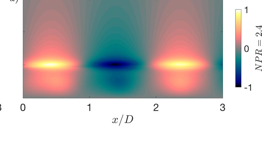
Absolute instability in shock-containing jets                          5
             p
and M = Mj Tj /T∞ is the acoustic Mach number, computed using the ideally expanded
jet Mach number Mj and the temperature ratio. The parameter δ defines the shear layer
thickness of the jet. It is worth noting that the oscillatory part of (2.4) is similar to
the one proposed by Tam & Tanna (1982) and Tam (1995) for the velocity variation
induced by the shock-cell structure. Equations (2.4) and (2.5) are considered as a first
approximation of the shock-cell structure, retaining some of its key characteristics, such
as streamwise dependence and some features of radial shape as derived by Pack (1950), at
least of the dominant term of the series that represents the shock-cell structure. Choice of
other radial shapes are expected to lead to similar results, as the streamwise periodicity
is the key element of this analysis, as will be shown in the next sections. The mean
streamwise velocity (and all other mean flow quantities) have an x-periodicity given by

                                 Ux (x, r) = Ux (x + N λsh , r),                            (2.6)
where N is an integer. Thus, (2.3) becomes a set of partial differential equations (PDEs)
with x-periodic coefficients. Following Herbert (1988) and Brevdo et al. (1996), such
periodicity allows us to use the Floquet ansatz and consider solutions in the shape

                                     q̂(x, r) = q̃(x, r)eiµx ,                              (2.7)
                                                                                   iµλsh
where q̃(x, r) has the same periodicity of the base flow. In this formulation e    is called
the Floquet multiplier, and µ = µr + iµi is the Floquet exponent. It is straightforward
to see that, for the locally parallel case, where q̃(x, r) = q̃(r), the Floquet exponent is
simply reduced to the streamwise wavenumber k in the normal mode ansatz. Due to its
periodicity in x, q̃(x, r) can be expanded as a Fourier series (Herbert 1988),

                                              ∞
                                              X
                                 q̃(x, r) =          q̃n (r)einksh x .                      (2.8)
                                              n=−∞
Thus, solutions related to the Floquet exponent µ+N ksh (with integer N ) can be written
as

                 ∞
                 X                                       ∞ h
                                                         X                       i
                        q̃n (r)einksh x eiµx eiN ksh x =     q̃n (r)ei(n+N )ksh x eiµx ,

    q̂(x, r) =                                                                              (2.9)
                 n=−∞                                    n=−∞

which means that solutions related to µ and µ + N ksh cannot be distinguished, as one
can be obtained from the other by simply reordering the Fourier coefficients.
  By substituting (2.7) into (2.3) we obtain

                                ∂              ∂q̃
                 − iωIq̃ + Lx     + iµ q̃ + Lr     + imLθ q̃ + L0 q̃ = 0,      (2.10)
                               ∂x              ∂r
which allows us to write an eigenvalue problem for the complex Floquet exponent,

                                          Lq̃ = Lµ µq̃.                                    (2.11)
The operators L and Lµ can be found in Appendix A.
  Equation 2.11 has exactly the same form as the locally parallel spatial stability analysis;
in fact, when µ = k both analyses are identical (as the streamwise derivatives in the
operators above can also be neglected in the local analysis). When Ash = 0, the solution
of the eigenvalue problem will give rise to modes following the relation µ = k + N ksh
in the eigenspectrum. However, if Ash > 0, i.e. the flow has a spatial variation within a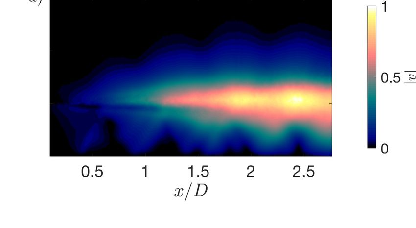
6                                  P. A. S. Nogueira et al.
wavenumber length, such modulation may change both the eigenvalues (related to phase
velocity and growth rate of the different waves supported by the flow), and the shapes
of the modes. Similar to the locally parallel case, downstream-travelling modes with
µi < 0 will be exponentially amplified in space (unstable modes), and all modes can be
classified by continuation from this previous case. The distinction between downstream-
(µ+ ) and upstream-travelling (µ− ) modes can be made by using Briggs’ criterion, as used
for parallel base flows (Briggs 1964; Tam & Hu 1989; Towne et al. 2017).
   The similarities between the present formulation and the locally parallel analysis
were further explored by Brevdo et al. (1996), who showed that the conditions for
absolute instability in spatially periodic flows are similar to the locally parallel case (as
summarised by Huerre & Monkewitz (1990)): the occurrence of a saddle point (related
to the appearance of a double root in the complex µ plane) for positive imaginary
frequency ωi > 0 is a condition for absolute instability. The impulse response of the
spatially periodic base flow at a fixed position x has an exp(−iω0 t) time dependence for
large t, where ω0 = ω0,r + iω0,i is the frequency of the saddle point. As in the locally
parallel case, the two modes involved in the saddle must also move to opposite sides of
the real µ axis for increasingly large ωi , which is the equivalent to the condition that
the saddle should be formed by a k + and a k − mode in this previous case. The saddle
with maximal ω0,i satisfying this condition is the relevant one for the calculation of the
impulse response, as it is the saddle point obtained with a continuous deformation of
the Fourier inversion contour starting from large ωi to ensure causality of the impulse
response (Huerre & Monkewitz 1990; Huerre 2000). This requirement is also equivalent
to the condition that the absolute value of the Floquet multipliers should move external
to the unit circle (|eiµλsh | = 1) for the first mode, and internal to this circle for the second
mode, in the limit ωi → ∞ (Brevdo et al. 1996). Essentially, writing the equations as
a function of the Floquet exponents leads to a linear problem that inherits most of the
characteristics of the locally parallel case (Brancher & Chomaz 1997); for this reason, it
will be analysed in the same fashion. The detection of a saddle point with ω0,i > 0 implies
that the impulse response of a spatially periodic base flow grows in both downstream and
upstream directions, leading to an oscillator behaviour with frequency ω0,r that spreads
throughout the domain. Around a fixed x, the spatial structure of the impulse response
at large t is given by the eigenfunction q̂(x, r) at the saddle point.
   The eigenvalue problem (2.11) is solved numerically by discretising the computational
field in the radial direction using Chebyshev polynomials, and in the streamwise direc-
tion using Fourier modes (Weideman & Reddy 2000). Radial mapping and boundary
conditions were implemented as in Lesshafft & Huerre (2007), and the problem was
solved numerically using the Arnoldi method (eigs in Matlab). For the cases studied
herein (especially for low Ash ), a discretisation of Nr × Nx = 80 × 31 in the radial
and streamwise directions was shown to be sufficient to converge all the relevant modes.
Computation of 400 eigenvalues using this number of points usually takes around 180
seconds on a standard laptop for each choice of parameters.

3. Results
   Depending on how far a jet is operated from its design condition, the shock and
expansion structures within the jet core can vary significantly in strength. Far from
the design condition, such as may be the case in rocket propulsion, the shock cells can
be complex structures, involving normal and oblique shocks, and their associated triple
points (Edgington-Mitchell et al. 2014a). Closer to the design point, where the nozzles of
air-breathing engines are likely to operate and screech is more likely to occur, the shock
Absolute instability in shock-containing jets                     7

Figure 1. Mean streamwise velocity for the N P R = 2.1 case normalised by the ambient sound
                       speed for Ash = 0 (a) and Ash = 0.02 (b).

structures are much weaker, and the compression and expansion may take place near-
isentropically. In the present analysis, we focus on two cases with relatively weak shocks
(nozzle pressure ratio N P R = 2.1 and 2.4 for convergent nozzles). Based on experimental
data at these conditions, a shock amplitude of Ash = 0.02 is selected to approximate the
oscillations observed around the fourth shock cell of these jets. Such shock amplitude
ensures that the entire region where the shocks are found in the flow is supersonic.
                                                                                p      As
in Pack (1950), the shock-cell wavelength is approximated by λsh = π/2.4048 Mj − 1,
where Mj is the ideally expanded jet Mach number. Previous results show that the first
case (N P R = 2.1) is dominated by an m = 0 (A1) screeching mode (Edgington-Mitchell
et al. 2018), and the second (N P R = 2.4) was shown to have a competition between
A2 (m = 0) and B (m = 1) modes (Li et al. 2020). Thus, the azimuthal wavenumbers
of the analysis were chosen as m = 0 for the first case, and m = 1 for the second. For
the absolute stability analysis, the shear-layer thickness was chosen as δ = 0.15 for the
m = 0 case, and δ = 0.25 for the m = 1 case. This is in line with the results of Powell
et al. (1992), who showed that screech B modes are associated with a larger jet spread
angle (see also Tan et al. (2017)). For the analysis of the modulation by the shock-cells,
δ = 0.15 was kept for both cases, in order to provide a fair comparison between the
effects of the shocks on the waves associated with both azimuthal wavenumbers.

                      3.1. Overall characteristics of the modulation
   We start by analysing the effect of the periodic shock-cell structure in the different
waves supported by the flow. Figure 1 shows the mean flows for Ash = 0 (equivalent
to the locally parallel case), and Ash = 0.02. Figure 1(b) exhibits some of the leading
characteristics of a shock-cell structure in an under-expanded jet, though with some
differences in shape when compared with experiments (see, for example, Edgington-
Mitchell et al. (2021a)). As noted by Tam & Tanna (1982), the addition of other shock-
cell wavenumbers may lead to a closer agreement in the shape of this structure with
experiments; here, we consider the leading wavenumber to be sufficient to analyse the
effect of such structure on the different waves in the flow. The only streamwise variations
allowed in the shear-layer are those arising from the presence of the shock-cell structure
in the flow.
   As a first test, the equivalence of the Ash = 0 case with the locally parallel linear
stability analysis (LSA) is demonstrated. To this end, the eigenspectrum for the N P R =
2.1, m = 0 case and Ash = 0 was compared to results from LSA using the same mean
flow and St = 0.7. The comparison between the eigenvalues is shown in figure 2, where
only 400 eigenvalues are shown. As expected, eigenvalues in the spectrum occur with a
ksh periodicity, such that µ = µ + N ksh , with N an integer; this is observed more clearly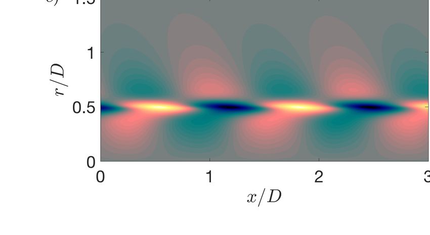
8                                P. A. S. Nogueira et al.

          5

          0

         -5

          -10            -5             0             5             10            15

Figure 2. Eigenspectrum containing 400 converged eigenvalues for N P R = 2.1, Ash = 0,
St = 0.7 (blue ). The eigenspectrum of the locally parallel analysis is also shown for µ = k
(orange +), µ = k − ksh (purple ×), and µ = k + ksh (yellow ×).

in the modes close to the imaginary axis (the acoustic branch), that also appear close to
µr = ksh , and in the unstable Kelvin-Helmholtz mode, now also present in the µr < 0
part of the spectrum due to this periodicity. Figure 2 also shows that the eigenvalues of
the locally parallel stability align perfectly with those from the periodic case, considering
the periodicity of the solution. Most modes could be captured by the LSA using µ = k
and µ = k ± ksh ; the few modes without equivalence seen on the real axis are related
to soft-duct modes of higher wavenumber (Towne et al. 2017). Due to the periodicity
of the solution, all modes from LSA are now observed inside the interval 0 6 µ 6 ksh .
Consequently, the identification of discrete modes and mode branches can be performed
directly by continuation from the locally parallel case.
   The introduction of a small value of Ash = 0.02 does not lead to significant changes
in the eigenvalues for the values of N P R analysed herein (variations in growth rate and
wavenumber are less than 0.01% for real-valued frequencies). However, the eigenfunctions
are non-trivially modified by the introduction of the shock-cell structure. Here, we analyse
this effect on two of the most dynamically significant waves in this flow. The first is the
Kelvin-Helmholtz (KH) mode (Michalke 1965), which is responsible for the appearance
of large scale vortical structures in the flow called wavepackets (Jordan & Colonius 2013),
one of the key structures responsible for sound radiation in turbulent jets (Cavalieri et al.
2019). The second is the upstream-travelling guided jet mode, first identified by Tam &
Hu (1989). Recent works (Gojon et al. 2018; Edgington-Mitchell et al. 2018; Mancinelli
et al. 2019) have shown that screech tones are observed within the frequency bands of
existence of these waves, at least for the axisymmetric mode, suggesting that this wave
might be responsible for closing the resonance loop in screeching jets. The presence of the
guided jet mode was also identified experimentally by Edgington-Mitchell et al. (2018,
2021a), which also highlights the importance of such waves in the dynamics of the jet. The
identification of these waves in the spatially periodic framework is less straightforward
than in the locally parallel case, especially for the guided jet mode. Due to the ksh
periodicity of the spectrum, this mode will now be mixed with critical layer modes and
soft-duct modes (Towne et al. 2017) on the µr axis. Since the eigenvalues for such small
Ash do not change relative to the Ash = 0 case, an auxiliary run of the locally parallel
case was used to identify the modes related to each wave.
   The real part of the streamwise velocity of both the Kelvin-Helmholtz and upstream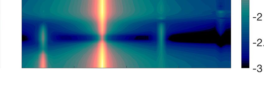
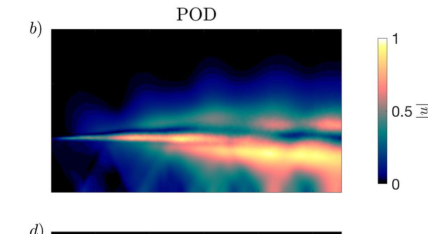
Absolute instability in shock-containing jets                        9

Figure 3. Real part of the streamwise velocity of the different waves analysed. Top:
Kelvin-Helmholtz (a) and upstream (b) modes for m = 0, N P R = 2.1 and St = 0.7. Bottom:
Kelvin-Helmholtz (c) and upstream (d) modes for m = 1, N P R = 2.4 and St = 0.47.
Spatially-periodic linear stability results for Ash = 0.02. The growth rates of the modes were
removed to allow for a better visualisation of the radial structure.

waves for m = 0, 1 and St = 0.7, 0.47 are shown in figure 3. The frequencies were
chosen to be within the frequency range of existence of the neutral guided jet mode
of radial order 2 and 1, respectively, and close to the screech frequencies observed in
these cases (see Edgington-Mitchell et al. (2018); Li et al. (2020)). Here, the modes are
reconstructed spatially using (2.7), and the imaginary part of the Floquet exponent
was ignored to better visualise the oscillatory behaviour of the modes. The shapes
of the Kelvin-Helmholtz modes follow the usual behaviour for m = 0 and m = 1
disturbances: in both cases, this wave is quite concentrated around the shear layer of
the jet (since the instability is driven by shear), and a phase jump around this position
is also observed. The differences between the m = 0 and m = 1 modes are observed
mainly around the centreline, where the helical modes should reach zero amplitude due
to their natural boundary conditions (Batchelor & Gill 1962). Both Kelvin-Helmholtz
modes depicted in figures 3(a,c) are comparable with the structures educed from a
proper orthogonal decomposition (POD) of experimental data, previously presented
in Edgington-Mitchell et al. (2018) (m = 0 dominated) and Edgington-Mitchell et al.
(2014b) (m = 1 dominated). The guided jet modes for the two cases are also shown in
figure 3 (b,d). These modes also follow the expected symmetry, being equivalent to the
ones presented by Gojon et al. (2018), for each azimuthal wavenumber and radial order.
   Figure 3 yields little insight regarding the effect of the shock-cell structure on the
different modes, since the modulation is masked by the phase evolution of the waves.
This effect can be seen more clearly by looking at the absolute value of the velocity for
each case. The locally parallel stability results lead to modes without any streamwise
variation in the absolute value of all flow quantities, while the spatially periodic case
allows the variation following the flow periodicity. This is shown in figures 4 (m = 0)
and 5 (m = 1) for the streamwise and radial velocity components. The changes in the
streamwise velocity of the axisymmetric modes induced by the inclusion of the periodic
10                               P. A. S. Nogueira et al.

Figure 4. Absolute value of the streamwise (a,c) and radial (b,d) velocities of the different
waves analysed for m = 0, N P R = 2.1 and St = 0.7. Kelvin-Helmholtz (a,b) and upstream
(c,d) modes for Ash = 0.02. The growth rates of the modes were removed to allow for a better
visualisation of the radial structure.

shock-cell structure are mainly concentrated around the centreline; the periodic shocks
have little effect around the shear layer. This changes when the radial velocity of the
Kelvin-Helmholtz is considered: modulation for this quantity actually occurs around the
shear layer. The modulation of the radial velocity for the upstream mode occurs between
the centreline and the first node in the radial direction (where the phase shift occurs).
   The behaviour of the modulated helical disturbances is shown in figure 5. For this
case, a slight modulation is observed in the streamwise velocity of the Kelvin-Helmholtz
mode, mostly around the shear layer and in the outer region of the jet. The modulation
is stronger in the radial velocity of the KH wave and in both components of the upstream
wave. Interestingly, different regions of the jet respond differently to the presence of the
periodic structure; while some regions of the jet follow the same oscillatory behaviour as
the shock-cell structure, other regions may follow the periodicity with a phase shift. This
is observed, for example, in figure 5(c), where disturbances around the shear layer follow
an inverse behaviour compared to disturbances at the centreline. Also, for both m = 0
and m = 1 disturbances, the modulation of the upstream-travelling waves is stronger
than for the Kelvin-Helmholtz mode.
   Figure 6(a) shows the modulation in streamwise velocity of both waves studied herein
for N P R = 2.1, m = 0, St = 0.7 and r/D = 0; the mean velocity at the centreline is also
shown for reference. All fields were normalised by their maximum and subtracted from
the initial value at x/D = 0. This plot shows clearly that the shock-cell structure has
opposing effects on the modulation of the different waves in the flow: while a maximum in
the mean velocity is associated with a maximum in the streamwise velocity of the Kelvin-
Helmholtz wave, it is also associated with a minimum of the guided jet mode. Considering
that these waves travel in opposite directions, this difference is possibly associated with
the effect of a wave passing through a shock coming from regions downstream or upstream
of it. Figure 6(a) confirms that the modulation effect is stronger in the upstream-travelling
wave for the m = 0 case. While the modulation of the guided jet mode is rather simple in
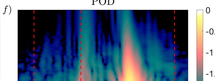
Absolute instability in shock-containing jets                      11

Figure 5. Absolute value of the streamwise (a,c) and radial (b,d) velocities of the different
waves analysed for m = 1, N P R = 2.4 and St = 0.47. Kelvin-Helmholtz (a,b) and upstream
(c,d) modes for Ash = 0.02. The growth rates of the modes were removed to allow for a better
visualisation of the radial structure.

shape, the modulation of the Kelvin-Helmholtz mode is more intricate. A slight oscillation
is observed around the mean point between a maximum and a minimum (or a node) of
the mean velocity, and a much stronger oscillation occurs at the position of minimum
velocity.
   A direct comparison between the present results and experiments is hard to perform.
Usually, the lack of time-resolved data only allows the identification of the structure
related to the resonance process (the screech mode) using proper orthogonal decom-
position or other similar modal decomposition tools (Edgington-Mitchell et al. 2014b,
2018; Li et al. 2020). However, the screech mode is composed of several downstream- and
upstream-travelling waves, which hinders the evaluation of such modulation effects in
the different waves of the flow. Still, considering that the screech mode is dominated by
a Kelvin-Helmholtz wavepacket, it could be expected that some of the trends identified
in the present study should be present in POD modes of experimental data. In order to
evaluate this, a complex mode is built using the two first POD modes, as in Edgington-
Mitchell et al. (2021a) for N P R = 2.1; the details about the experiments and numerical
procedure can be found in the cited paper. The streamwise evolution of the screech
mode at the centreline is shown in figure 6(b), where the mean velocity is also shown as
reference. Comparing figures 6(a) and (b), some similar features can be identified. As in
the spatially-periodic analysis, the POD mode also has maxima in streamwise velocity
aligned with maxima in the mean velocity (maxima of the shock-cell structure). Also,
oscillations following the same pattern are observed around the third shock-cell, both
associated with nodes and minima in the mean velocity. Considering a spatial growth
of the KH mode enhances the comparison, as shown in figure 6(c). However, there is
no reason to expect quantitative agreement in growth rate between an inviscid, linear,
periodic model and the experimental data; indeed, there is a significant difference between
the values. As the purpose of this figure is purely to illustrate similar trends in the
modulation effect, the growth rate of the KH mode is reduced to 20% of its value for the
12                                  P. A. S. Nogueira et al.
     0.2

     0.1

       0

     -0.1

     -0.2
            0   0.2     0.4     0.6          0.8       1       1.2   1.4     1.6       1.8     2

        1

      0.8

      0.6

      0.4

      0.2

        0
            0    1      2       3        4         5       0   0.5   1     1.5     2     2.5

Figure 6. Comparison between the modulation of the different waves in the spatially periodic
linear stability analysis and the POD mode from Edgington-Mitchell et al. (2018) at the
centreline (r/D = 0) and N P R = 2.1. The spatially periodic modes (a) are normalised by
their maximum and subtracted from their value at x/D = 0, and the imaginary part of the
Floquet exponent was ignored in the spatial reconstruction of the modes. In (b), the POD
mode and mean streamwise velocity are normalised by their maximum. The mean velocity and
the spatially growing KH mode (growth rate reduced to 20% of its original value) (c) are also
normalised by their maximum.

purpose of this comparison. Overall, considering that the only spatial evolution allowed
in the present model is the periodic shock-cell structure, the present model captures some
of the experimental trends quite closely, supporting the use of the present tool in the
analysis of shock-containing flows.

                        3.2. Saddle points and absolute instability
  In the previous section, we showed that the spatially periodic linear stability analysis
manages to capture some of the trends identified in experiments. We also showed that
results from this formulation can be analysed in the same fashion as the locally parallel
case, with modes categorised in a very similar manner to this previous method; in fact,
for Ash = 0, the present method recovers the exact same modes as the local analysis.
As mentioned in the previous section, small changes in the growth rates and peak
wavenumber were identified for Ash = 0.02. Thus, one could erroneously think that
the only effect of such flow periodicity is on the shapes of the different waves supported
by the flow. In this section we show that this is not the case. In fact, the periodicity
Absolute instability in shock-containing jets 13
0
Guided jet
mode
-0.5
KH mode
-1
-1.5
6.5 7 7.5 8
Figure 7. Trajectories of the different modes in the complex µ plane, for N P R = 2.1, m = 0,
Ash = 0.02 and St = 0.685, for several values of ωi .
changes the nature of the instability mechanism to which the flow is subject, and this
will have a direct effect on the physical interpretation of the screech phenomenon.
In the present section, we follow the formulation developed by Huerre & Monkewitz
(1985), revised in Huerre & Monkewitz (1990), and extended to spatially periodic base
flows in Brevdo et al. (1996). For a clearer interpretation of the results of Brevdo et al.
(1996), the reader can also refer to Brancher & Chomaz (1997). In summary, an absolute
instability occurs if a saddle in the (ω, µ) plane exists for ω0,i > 0, and this saddle must
be formed between an upstream- and a downstream-travelling mode. Considering that all
waves are now in the same region of the spectrum (between 0 6 µr 6 ksh ), an interaction
between downstream- and upstream-travelling waves is more likely to occur. In order to
evaluate this, the complex frequencies ω in which the complex eigenvalue related to the
Kelvin-Helmholtz mode approaches the eigenvalue of an upstream travelling wave were
sought for the locally parallel case. Then, second and third runs of the spatially periodic
stability were performed for Ash = 0 and Ash = 0.02, in order to evaluate the effect
of the mean flow periodicity, checking if the shock-cell structure leads to an interaction
between the different modes. In the parametric studies, saddles were sought using the
methodology proposed by Monkewitz (1988).
The effect of increasing ωi in the eigenspectrum is exemplified in figure 7. The Kelvin-
Helmholtz mode is directly identified as the only unstable mode (µi < 0) for ωi = 0.
As expected for an unstable downstream-propagating mode, increasing ωi leads to an
increase in the value of µi ; for larger imaginary frequencies, this mode will cross the real
axis and remain in the µi > 0 region of the spectrum. The opposite happens with the
guided jet mode, identified as the discrete mode closest to the continuous neutral acoustic
branch for ωi = 0. Since this mode is upstream propagating, increasing the imaginary
frequency leads to a decrease in µi . The contrasting behaviour of these two modes leads
them to be located quite close to each other for some values of ωi , which could allow for
an interaction between the downstream- and upstream-travelling modes.
The trajectories of the eigenvalues related to Kelvin-Helmholtz (KH) and guided-
jet/upstream (Ups) modes in the complex µ plane for increasing St number are shown
in figure 8. These trajectories were computed for ωi = {0.436, 0.446} (m = 0) and ωi =
{0.180, 0.204} (m = 1), and in the interval 0.682 6 St 6 0.689 and 0.442 6 St 6 0.452
respectively. In both figures 8(a,b), KH modes travel from left to right for increasing St,
and upstream modes move from right to left. For Ash = 0, the trajectories of both modes
approach each other, but continue straight in their original path; considering that the14 P. A. S. Nogueira et al. Ash = 0 case is exactly equivalent to the locally parallel case (except for the periodicity of the modes in the complex µ plane), this is not surprising: no absolute instability is observed between these two modes, as they originally inhabited different regions of the spectrum in the locally parallel case. As the periodicity is included (Ash = 0.02), the trajectories of these modes deform around a given point µs of the spectrum. Close to this point, both modes move towards each following a specific direction, and are repelled in a perpendicular direction for higher St. This is a direct symptom of a double root in the µ(ω) relation, characterising a saddle point. As in the locally parallel case, these two waves move in opposite directions of the real µ-axis for increasingly large ωi , being equivalent to k + (KH mode) and k − (upstream mode) waves (see Huerre & Monkewitz (1990) for more details). In the spatially periodic framework, this also means that for ωi → ∞, one of the modes travels internally to the unit circle for the Floquet multiplier (|eiµλsh | = 1) and the other travels externally to that circle. These two conditions, associated with the fact that the saddles occur for ω0,i > 0, define the absolute instability of a spatially periodic system, as derived by Brevdo et al. (1996). Thus, the impulse response of the spatially periodic shock-cell pattern grows in both downstream and upstream directions, leading to an oscillator behaviour that spreads throughout the domain for large times. Considering that these modes have similar trajectories for several values of ωi , this phenomenon occurs twice for this periodic flow: once when the KH mode is on the bottom part of the spectrum (low ω0,i , figures 8(a,b)), and again when this mode is at the top part of the spectrum (higher ω0,i , figures 8(c,d)). These two saddles are formed by the same modes, and are very close to one another. The spatio-temporal growth rates associated with these are also similar, suggesting that both saddles are representative of the same phenomenon. With that in mind, mode shapes and wavenumber spectra displayed in the remainder of this paper are related to the second saddle (higher ω0,i ), as it dominates the impulse response of the flow for large t. An interaction between the KH mode and a mode from the acoustic continuous spec- trum is also observed in figure 8(c). Given that the upstream component of screech was historically assumed to be characterised by free stream acoustic waves, such interaction may at first seem of significance. However, care must be taken in its interpretation for a number of reasons. Modes from this branch are discrete representations of a continuous branch associated with sound waves radiating in several directions (Gloor et al. 2013), and are related to a branch cut in the Briggs-Bers analysis, as shown by Huerre & Monkewitz (1985). In this previous work, the authors have also shown that the contribution of this continuous branch decays exponentially for large times, and was neglected in the absolute instability analysis. Also, as the KH and guided jet modes switch identities at the saddle, it is hard to determine if the interaction between the discrete mode and the acoustic branch is formed between downstream- and upstream-travelling waves; thus, such interaction may be entirely due to the partial identification of this mode as a guided jet mode, which ejects from the acoustic branch for a given frequency (see Towne et al. (2017)), and may still be able to interact with such branch. No saddle with acoustic modes was found for imaginary frequencies far from the saddles related to the guided jet mode. Figures 8(a-d) show that saddle-points between Kelvin-Helmholtz and guided jet modes can be found in spatially periodic flows, such as shock-containing jets; unlike for the ideally expanded case where an absolute instability is only observed in low-density jets (Monkewitz & Sohn 1988), the presence of a periodic structure, such as the train of shock-cells, can allow for the interaction of modes that could not interact in the locally parallel framework. The connection between the present absolute instability mechanism and screech can be accessed by the analysis of both the frequency of the saddle (or the
Absolute instability in shock-containing jets                               15
                                                         -0.22
  -0.47
                                                         -0.24

  -0.48
                                                         -0.26

  -0.49                                                  -0.28

    -0.5                                                  -0.3
       7.1   7.12    7.14    7.16     7.18         7.2                 4.4          4.45         4.5

                                                         -0.24
  -0.46

                                                         -0.26
  -0.47

                                                         -0.28
  -0.48

                                                          -0.3
  -0.49
                                                         -0.32
      7.1    7.12   7.14    7.16    7.18     7.2                 4.4         4.45          4.5

Figure 8. Trajectories of the Kelvin-Helmholtz (KH) and guided jet (Ups) modes in the complex
µ plane, for both m = 0 (a,c) and m = 1 (b,d) cases, for ωi = 0.436 (a), ωi = 0.180 (b),
ωi = 0.446 (c) and ωi = 0.204 (d). Modes are shown in the interval 0.682 6 St 6 0.689 for the
axisymmetric case, and 0.442 6 St 6 0.452 for the helical case. All modes are named according
to their identity at the lowest Strouhal number in each plot. In (c), the trajectory of a mode
from the continuous acoustic spectrum (Ac) is also shown.

N P R Spatially periodic analysis Experiments/Simulation            Reference
 2.1         St0 ≈ 0.684             Stscreech = 0.67    Edgington-Mitchell et al. (2018)
 2.4         St0 ≈ 0.447            Stscreech = 0.4237           Li et al. (2020)
 Table 1. Approximate frequencies of the saddle in the spatially periodic analysis compared
                 with screech frequencies from simulations/experiments.

frequency of interaction between the two modes), and the shapes of the modes close to
the saddle, keeping in mind the approximations of the current model. Table 1 shows the
comparison between the frequencies of the saddles, reported in terms of the Strouhal
number St0 = ω0,r /(2πM ), for both m = 0 and m = 1 cases, and the experiments
of Edgington-Mitchell et al. (2018) and simulations of Li et al. (2020). Interestingly,
the frequencies predicted by the spatially periodic analysis are quite close to the ones
from these previous works, for both values of N P R and azimuthal wavenumbers. This
agreement supports the hypothesis that the absolute instability mechanism captures
some features of the screech phenomenon, and that the frequency of the resonance loop
is actually given by the frequency where the saddle point is identified.
   The sensitivity of the temporal growth rates and Strouhal number to the shock
16 P. A. S. Nogueira et al.
amplitude is shown in figure 9(a,b). As suggested by the results in figures 8(a,c), the
difference in frequency between the two saddles is small for Ash = 0.02; figures 9(a,b)
show that this difference decrease as Ash is decreased, and the two saddles coalesce for
vanishing values of shock-cell amplitude. No saddle is observed for Ash = 0, which points
to the absence of absolute instability in the locally parallel case. Overall, both temporal
growth rates and Strouhal number of the saddle are fairly insensitive to changes in
shock-cell amplitude, as shown in figures 9(a,b). On the other hand, these quantities are
strongly affected by the shear-layer thickness δ. Figure 9(c) shows a monotonic decrease
in the growth rates of the structures associated with both saddles as δ increases, which
is in line with the decrease in the spatial growth rate of the Kelvin-Helmholtz mode with
increase of shear-layer thickness (Michalke 1984). The Strouhal numbers associated with
the saddle increase slightly with the increase of δ, but these values still remain in the
frequency range where screech is expected to occur for this value of N P R (Mancinelli
et al. 2019).
These results altogether suggest that a pocket of absolute instability, obtained in a
periodic stability analysis using velocity profiles from various x stations, might be present
in real shock-containing flows, where the jet spreading will have a stabilising effect on
the disturbances. This is also similar to the studies of pockets of absolute instability in
wakes (Chomaz et al. 1988). Still, differently from the wake case, the absolute instability
in shock-containing jets is triggered by the periodicity induced by the shock-cells, and no
pocket of absolute instability is observed for such jets in the locally parallel framework.
We emphasise that, contrary to former models that needed empirical inputs, the absolute
instability analysis in the spatially periodic framework predicts the screech frequencies
directly as a function of the jet operating condition. Increasing the shear-layer thickness
leads to small variations on the predictions within the range of frequencies in which
screech is observed. No other input from experiments is needed.
3.3. Comparison of absolute instability eigenfunctions with data
Further analysis of the structure of the modes close to the the resonant condition may
confirm if the absolute instability mechanism is actually representative of the screech
phenomenon. Here, we wish to discern if the large-time response to an impulse applied
to a spatially-periodic shock cell pattern resembles the dominant coherent structures in a
screeching jet. The axisymmetric modes for N P R = 2.1, St = 0.6841 and ωi = 0.4465 are
presented in figure 10(a,c), where the absolute value of streamwise and radial velocities
are shown, respectively. The spatial growth of SP-LSA modes is also included in the
reconstructions. Comparing figures 10(a,c) to figures 4(a-d), it is clear that the effect
of the modulation by the shock-cell structure is minor close to the resonant condition
(which may be related to the spatial distribution of the modes further downstream in
figure 6(b)), and the interference pattern between the two waves involved in the saddle is
now dominant. This interaction leads to strong modulation of the resulting wavepacket
structure throughout the domain (Edgington-Mitchell et al. 2021a). The structure of the
modes close to the saddle can also be compared to the most energetic coherent structure
coming from a POD of experimental data, presented in Edgington-Mitchell et al. (2018)
and Edgington-Mitchell et al. (2021a), shown in figures 10(b,d). Even though the modes
from the spatially periodic analysis do not capture the growth/decay behaviour of the
wavepacket (which is due to the increasing shear-layer thickness, not included in the
model), the overall modulation pattern is quite well reproduced by the modes. Such
agreement can be especially observed close to the centreline and outside the shear layer,
where a wavy pattern is clearly seen. The POD modes are also more radially spread
across the shear layer and potential core, which is also likely due to the jet spreading.Absolute instability in shock-containing jets 17
0.6846
0.446
0.6845
0.444
0.6844
0.442
0.6843
0.44
0.6842
0.438
0.6841
0.436
0.684
0 0.005 0.01 0.015 0.02 0 0.005 0.01 0.015 0.02
0.5 0.7
0.4
0.695
0.3
0.69
0.2
0.685
0.1
0 0.68
0.16 0.18 0.2 0.22 0.16 0.18 0.2 0.22
Figure 9. Imaginary frequency ω0,i (a,c) and Strouhal number St0 (b,d) of the first and second
saddle points for N P R = 2.1 and m = 0 as a function of shock amplitude Ash and shear layer
thickness δ. Results for δ = 0.15 (a,b) and Ash = 0.02 (c,d).
The spatial reconstruction of the m = 1 mode for N P R = 2.4, St = 0.448 and
ωi = 0.204 is shown in figures 11(a,c). As in the axisymmetric case, the interference
pattern formed by the interaction between the two waves is much stronger than the
modulation by the shock-cell structure alone. Compared to the non-resonant condition,
changes in the mode structure are also seen over the entire mode, especially for the radial
velocity; in this velocity component, an alternation of peak velocities around the shear-
layer and centreline is observed as consequence of the regions of the peak of each wave
(as shown in figures 5(b,d)) and the interference pattern. The only modal decomposition
data available for this operating condition are the DMD modes presented by Li et al.
(2020), where only the real part of the modes are shown, hindering the identification
of the modulation. Thus, a comparison with modes from another operating condition
(N P R = 3.4, studied in Edgington-Mitchell et al. (2014b) and Edgington-Mitchell et al.
(2021a)) is performed here. Even though the flow for this higher Mach number case is
slightly more complicated (especially considering the presence of a small Mach disk) it
is also dominated by an m = 1 screeching mode, as in the present case. It is also worth
highlighting that the shock-cell wavelength for this higher N P R case is larger, so the
modulation wavenumber of the mode close to the saddle will differ from the experimental
result; thus, only qualitative comparisons about the structure of the resonant mode may
be performed in this case. The absolute value of the streamwise and radial velocities for
this case are shown in figures 11(b,d). As in the axisymmetric case, a good agreement
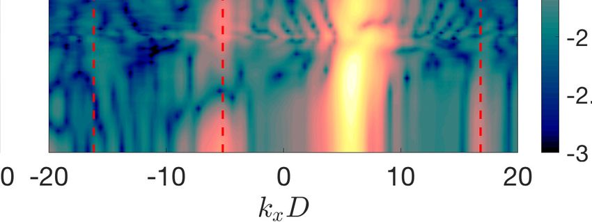
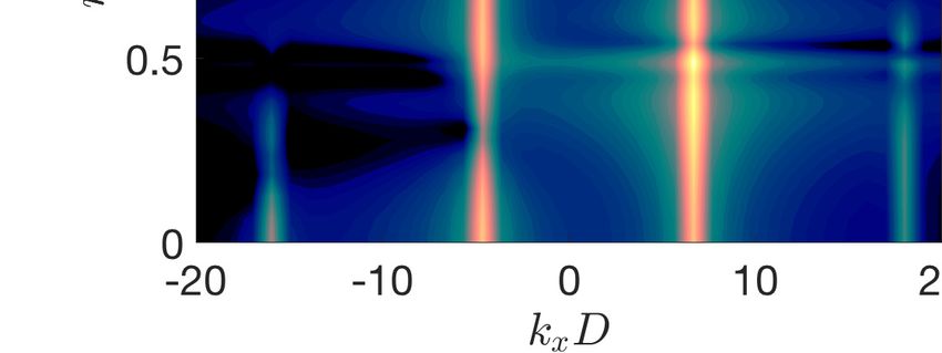
between the structure of the spatially periodic modes and the POD modes is obtained18 P. A. S. Nogueira et al. Figure 10. Comparison between the shapes of the modes close to the saddle and POD modes for N P R = 2.1 and m = 0. The spatial growth rates of the modes (µi ) are now included in the reconstruction. Absolute value of streamwise and radial velocities are shown in (a) and (c) for the spatially periodic stability analysis, and streamwise and lateral velocities of the POD modes (N P R = 2.1) reported in Edgington-Mitchell et al. (2021a) are shown in (b) and (d). All modes are normalised by their maximum. for m = 1 disturbances. The wave-interaction pattern follows the experimental data quite closely, especially in the outer region of the jet, for the streamwise velocity. For this component, the viscous effects and the shear-layer development also lead to modes more radially spread. A remarkable agreement for the radial velocity is observed, with both fields following the particular peak-shift behaviour between the centreline and the shear-layer. The presence of both KH and upstream waves in the mode at the saddle point can be more clearly observed in the analysis of the wavenumber spectrum of this mode. The streamwise velocity of the modes are reconstructed in the first ten shock-cells ignoring the spatial growth rate (µi ), in order to isolate the oscillatory behaviour of the modes. It is desirable to evaluate the streamwise wavenumbers present in the eigenfunctions of each wave as one approaches the saddle; thus, a spatial Fourier transform of the reconstructed mode is performed for different values of ωi . This analysis is equivalent to the one performed by Edgington-Mitchell et al. (2021a) on POD and global stability modes. Considering that only wavenumbers µr + N ksh are allowed in each mode, the spatial spectra provides a good estimate of the relative energy of the different wavenumbers included in each mode, allowing for a clearer identification of the different waves at the saddle point. Figures 12(a-d) show the wavenumber spectra of the modes related to the KH (a,c) and guided jet (b,d) waves for ωi = 0, 0.4. These plots show the energy content of each wavenumber of the reconstructed mode using a fast Fourier transform (fft). The discrete wavenumbers allowed in the eigenfunctions will appear as most energetic; energy in wavenumbers other than µr + N ksh must be disregarded, as it is related to contour interpolation and to the truncation of the domain for the fft, as the wavenumbers λsh and 2π/µr are not multiples of each other. For zero imaginary frequency, both modes have peaks at the expected wavenumbers (positive for the KH, negative subsonic for
Absolute instability in shock-containing jets                         19

Figure 11. Comparison between the shapes of the modes close to the saddle and POD modes
for N P R = 2.4 and m = 1. The spatial growth rates of the modes (µi ) are now included in the
reconstruction. Absolute value of streamwise and radial velocities are shown in (a) and (c) for
the spatially periodic stability analysis, and streamwise and lateral velocities of the POD modes
(N P R = 3.4) reported in Edgington-Mitchell et al. (2021a) are shown in (b) and (d). All modes
are normalised by their maximum.

the guided jet mode), and small energy peaks related to the modulation analysed in
section 3.1 are also observed. As the imaginary frequency is increased to ωi = 0.4, the
energy of wavenumbers related to upstream waves start to increase in the KH mode
(and equivalently in the upstream wave), until both modes become one at the saddle
point. There, it is impossible to separate both waves, and the resulting mode has energy
peaks at the wavenumbers of both waves, as shown in figure 12(e). At this position, both
modes share the same eigenvalue µ, and only wavenumbers k = µr + N ksh are allowed
in the eigenfunction. Hence, the wavenumbers of both waves that compose the saddle
must observe the relationship kkh − ksh = kupstream , where kkh , kupstream are the peak
wavenumbers of the KH and upstream waves (associated with N = 0, −1, respectively),
identified by a continuation of the wavenumber spectra from ωi = 0 to ωi = ω0,i . This
is exactly the wavenumber relation derived by Tam & Tanna (1982), and confirmed
You can also read