Simulating quantum many-body dynamics on a current digital quantum computer - mediaTUM
←
→
Page content transcription
If your browser does not render page correctly, please read the page content below
www.nature.com/npjqi

                  ARTICLE                   OPEN

                  Simulating quantum many-body dynamics on a current digital
                  quantum computer
                                    1,2*
                  Adam Smith               , M. S. Kim1, Frank Pollmann2 and Johannes Knolle1

                     Universal quantum computers are potentially an ideal setting for simulating many-body quantum dynamics that is out of reach for
                     classical digital computers. We use state-of-the-art IBM quantum computers to study paradigmatic examples of condensed matter
                     physics—we simulate the effects of disorder and interactions on quantum particle transport, as well as correlation and
                     entanglement spreading. Our benchmark results show that the quality of the current machines is below what is necessary for
                     quantitatively accurate continuous-time dynamics of observables and reachable system sizes are small comparable to exact
                     diagonalization. Despite this, we are successfully able to demonstrate clear qualitative behaviour associated with localization
                     physics and many-body interaction effects.
                     npj Quantum Information (2019)5:106 ; https://doi.org/10.1038/s41534-019-0217-0
1234567890():,;

                  INTRODUCTION                                                                          example, allowed us to study Hubbard model physics31,35 and
                  Quantum computers are general purpose devices that leverage                           many-body localized systems32–34 in two dimensions. More
                  quantum mechanical behaviour to outperform their classical                            recently, there have also been advances in trapped ion quantum
                  counterparts by reducing the computational time and/or the                            simulators, which have the benefit of being able to implement
                  required physical resources.1 Excitement about quantum compu-                         long range interactions,6,7,37 and have been used to study the
                  tation was initially fuelled by the prime-factorization algorithm                     Schwinger-mechanism of pair production/annihilation in 1D
                  developed by Shor,2 which is most popularly associated with the                       lattice QED7 and Floquet time crystals.38
                  ability to attack currently used cyber security protocols. More                          Universal quantum computers are also increasingly looking like
                  importantly, it provided a paradigmatic example of dramatic                           a feasible setting for simulating quantum dynamics. One of the
                  exponential improvement in computational speed when com-                              biggest advantages of using a quantum computer for this purpose
                  pared with classical algorithms. It has since been realised that the                  is the flexibility it offers. A single quantum device could in
                  potential power of quantum computers could have far reaching                          principle perform simulations that currently require several
                  applications, from quantum chemistry and the associated benefits                       different experiments, using disparate methods. Furthermore, it
                  for medicine and drug discovery,3 to quantum machine learning                         should be possible to access new physics not currently accessible,
                  and artificial intelligence.4 Even before reaching these lofty goals,                  most notably, the simulation of lattice gauge theories with
                  there may also be practical uses for noisy intermediate-scale                         dynamical gauge fields. These are ubiquitous in the theoretical
                  quantum (NISQ) devices.5                                                              study of strongly-correlated quantum matter but require multi-
                     These quantum devices can be implemented in a large number                         body couplings, which have so far proven difficult to achieve in
                  of ways, for example, using ultracold trapped ions6–11 cavity                         experiment.39,40
                  quantum electrodynamics (QED),12–15 photonic circuits,16–18 sili-                        A particularly exciting opportunity has been provided by IBM in
                  con quantum dots,19–21 and theoretically even by braiding, as yet                     the form of an online quantum computing network called IBM Q.
                  unobserved, exotic collective excitations called non-abelian any-                     This consists of a set of small quantum computers of 5 and 16
                  ons.22–24 One of the most promising approaches is using                               qubits that are available freely to the public, two 20 qubit
                  superconducting circuits,25–27 where recent advances have                             machines accessible by IBM Q partners,41 and the qiskit python
                  resulted in devices consisting of up to 72 qubits, pushing us ever                    API42 for programming the devices. The publicly available
                  closer to realising so-called quantum supremacy.28 The apparent                       resources have already resulted in a spread of results, such as
                  proximity of current devices to this milestone makes it timely to                     calculating the ground state of simple molecules,3,43 creating and
                  review the current capabilities and limitations of quantum                            measuring highly entangled many qubit states,44,45 implementing
                  computers.                                                                            quantum algorithms,46–48 and simulating non-equilibrium
                     Richard Feynman’s original idea was to simulate quantum                            dynamics in the transverse-field Ising,49,50 Heisenberg51,52 and
                  many-body dynamics—a notoriously hard problem for a classical                         Schwinger53 models, as just a few examples. Given the infancy of
                  computer—by using another quantum system.29 Over the last                             quantum computing efforts, all these results are understandably
                  couple of decades, this approach of using a purpose built                             small scale and of limited accuracy.
                  quantum simulator has been extremely successful in accessing                             IBM is not alone in their efforts to make quantum computing
                  physics beyond the reach of numerics on a classical computer.                         more mainstream, with Microsoft introducing the Q-sharp
                  Most notable are cold atom experiments with optical lattices30–36                     programming language,54 Google developing the Circq python
                  where the natural evolution of the atoms corresponds to a high                        library,55 and Rigetti providing their own Quantum Cloud Service
                  accuracy to that of a local Hamiltonian of choice. This has, for                      and Forest SDK built on Python.56 Rigetti and IonQ also provide

                  1
                   Blackett Laboratory, Imperial College London, London SW7 2AZ, UK. 2Department of Physics, T42, Technische Universität München, James-Franck-Straße 1, D-85748 Garching,
                  Germany. *email: adam.smith@tum.de

                  Published in partnership with The University of New South Wales
A. Smith et al.
2
selective public access to hardware—based on superconducting
qubits and trapped ions, respectively. All of these resources are
allowing a lot of hands on experience with quantum computers
from researchers and the general public all around the world.
Furthermore, it highlights that there are currently several parallel
efforts of research and development from industry focussed on
quantum computing, quantum programming and cloud-based
services that are flexible and prepared for future hardware.
Given the current stage of development, and the immense
expectation from the public and physics communities, it is timely
to critically assess and benchmark the state-of-the-art. In this
article we consider the far-from-equilibrium dynamics of global
quantum quenches simulated on an IBM 20 qubit quantum
computer. The models that we consider are of central importance
to condensed matter physics and display a wide range of
phenomenologies. By measuring a range of physical correlators, Fig. 1 Schematic of the implementation of Trotterized evolution. a The
procedure of adding more Trotter steps to reach longer times. b, c
we can assess the capabilities and limitations of current quantum are the basic and symmetric Trotter decomposition, respectively, for
computers for simulating quantum dynamics. ^j ¼ eihj σ^j Δt ;
z
^j ¼
the Hamiltonian Eq. (3). In b the operators are A B
^ ^ ^ ^ ^j ¼
z z x x y y
iðU^σ j σ jþ1 Jð^ σ j σjþ1 þ^ σ j σ jþ1 ÞÞΔt ^ zj Δt
ihj σ
e and in c they are Aj ¼ e 2 ; B
^ zjþ1 Jð^ σ j σ^jþ1 ÞÞΔt
^xjþ1 þ^ ^ ^ zjþ1 Jð^
σ xj σ^xjþ1 þ^ ^ jþ1 ÞÞΔt
y y y y
iðU^σ zj σ σ xj σ σzj σ
iðU^ σj σ
RESULTS e 2 ; Cj ¼ e .
Setup
In this article, we study global quantum quenches,57,58 that is we
calculate local observables and correlators of the form These Hamiltonians are perfect testbeds for digital quantum
simulation since they can be directly simulated on a quantum
ψðtÞO^ j ψðtÞ ; ψðtÞO ^ k ψðtÞ ;
^jO
1234567890():,;
(1)
computer – the spins-1/2 of the former correspond directly to the
where O ^ j are local operators and the time-dependent states are qubits of the latter, and the local connectivity of the qubits is
^ suited for the local form of the Hamiltonian.
jψðtÞi ¼ eiHt jψð0Þi; (2) In our simulations we achieve the time evolution using a Trotter
and where jψð0Þi is the initial state, which differs globally from an decomposition66,67 of the unitary time evolution operator
^ ¼ eiHt ^
eigenstate of H. ^ In other words, we can consider jψð0Þi to be the UðtÞ . Our simulation proceeds by the following steps.
ground state of a (time-independent) preparation Hamiltonian, First, we create the initial state, which is done by applying Pauli-X
^0 ¼ H
H ^ hV,
^ where V^ is a global perturbation, and the perturba- operations to the default initial state of the IBM machine,
tion strength h is instantaneously quenched from zero at time j """ i. Second, we discretize time and the evolution
t ¼ 0. becomes a product of discrete evolution operations
^ ¼ UðΔtÞ
UðtÞ ^ ^
UðΔtÞ. Note that in our plots we include
We consider one dimensional spin-1/2 chains, consisting of N
spins, initially prepared in either a domain wall configuration, additional data points by varying δt in the final discrete evolution
j ###""" i, or Néel state, j "#"#" i. Quenches from step. Third, we trotterize the discrete operators UðΔtÞ into a
these initial states are particularly easy to prepare due to the local product of one- and two-qubit unitaries. Finally, we decompose
tensor-product structure of the initial state and have been studied these unitaries into the CNOT and single qubit rotation gates that
in cold atom experiments.32 The time evolution after the quantum can be directly applied on the IBM devices. Please see Fig. 1 for a
quench will be governed by a Hamiltonian of the form schematic of this procedure, and see Methods for more details.
Once we have constructed the state jψðtÞi, we then perform
N1
X X
N1 X
N
^ ¼ J measurements, which allows us to construct the quantities of
H σ^ xj σ^ xjþ1 þ σ^ yj σ^ yjþ1 þ U σ^ zj σ^ zjþ1 þ hj σ^ zj ; (3) interest in Eq. (1). We will only consider correlators of σ^ zj operators,
j¼1 j¼1 j¼1
where we only need to make measurements in a single (z-basis) for
with J > 0, and σ^ αj
are the Pauli matrices with eigenvalues ±1. This the spins. In the following we will use 8192 measurements per data
model can also be written in terms of hard-core boson, or spinless point, which means that the statistical error for these local
fermion Hamiltonian via the Jordan-Wigner transformation. correlators is 0:01, which is too small to be included in our figures.
We will consider four distinct cases for the Hamiltonian We consider three different types of dynamical quantities:
parameters:
● The local magnetization
(i) The XX chain, defined by U ¼ 0 and hj ¼ 0. This is a uniform,
Mj ðtÞ ¼ hψðtÞjσ^ zj jψðtÞi: (4)
non-interacting model.
(ii) Disordered XX chain for U ¼ 0 and hj uniformly randomly In the case of a domain wall initial state, we will also compute
sampled from the interval ½h; h. This is the prototypical
lattice model for Anderson localization.59 X
N=2
^ zj þ 1
σ
Nhalf ðtÞ ¼ hψðtÞj jψðtÞi; (5)
(iii) XXZ spin chain, defined by U ≠ 0 and hj ¼ 0. This is a j¼1
2
particular case of the Heisenberg model for quantum
magnetism. which is equal to zero at t ¼ 0 and grows as the domain wall
(iv) XXZ chain with linear potential, defined by U > 0 and hj ¼ hj, spreads.
● The connected equal-time correlator
i.e., a linearly increasing potential. This model was recently
studied in the context of many-body localization without C jk ðtÞ ¼ hψðtÞjσ^ zj σ^ zk jψðtÞi hψðtÞjσ^ zj jψðtÞihψðtÞjσ^ zk jψðtÞi:
disorder,60,61 where Wannier-Stark localization62 is induced
by the linear potential. (6)
This family of Hamiltonians covers a large range of physics in Note, the connected form of this correlator measures the
condensed matter, from the integrable limit,57 to many-body quantum correlators between distant spins but is not sensitive
quantum magnetism,63 to that of many-body localization.64,65 to the classical correlations in our initial states.
npj Quantum Information (2019) 106 Published in partnership with The University of New South WalesA. Smith et al.
3
Fig. 2 Results for a global quench from a domain wall initial state. a, b The local magnetization of the fourth and sixth spins of the chain with
N ¼ 6, and c is for the sixth spin for longer times. Plotted are the result of exact diagonalization, numerical Trotter evolution, and the
experimental data, both in raw form (IBM) and when the conserved quantities are imposed (IBM constrained), see the main text. d–f The time
and site resolved IBM results for the local magnetisation for N ¼ 6; 8; 10 sites, respectively. g The corresponding numerical symmetric Trotter
evolution for N ¼ 10. Data were obtained on 12 March 2019 for all figures except (c), which were obtained on 3 April 2019.
● The quantum Fisher information (QFI). We will consider a is that the fidelities of these two qubit gates are an order of
particular case of the QFI for a pure state, namely, magnitude worse than the single qubit gates. The CNOTs also take
!2 a longer real-world time to implement than the single qubit gates.
X X The increased implementation time of the circuits increases the
F Q ðtÞ ¼ sj sk hψðtÞjσ^ j σ^ k jψðtÞi
z z
sj hψðtÞjσ^ j jψðtÞi ;
z
jk j
potential for errors due to energy relaxation and dephasing,
parametrized by the T1 and T2 times, as well as other
(7) environmental effects and cross-talk. On the IBM device, we use
where sj ¼ þ1 for left half of the sites j and sj ¼ 1 for the N = 6, 8, 10 of the qubits as our system with 4 or 5 symmetric
right half at t ¼ 0. More generally, the QFI (for a pure state) is Trotter steps. These qubits are chosen as the connected subset
defined as the variance, 4ðhO ^ 2 Þ, where O
^ 2 i hOi ^ is a sum of with the lowest average CNOT errors such that the single qubit
local operators, which each have a spectrum of unit width. In measurement errors and T2 decoherence times do not exceed a
our case we have O ^ ¼ 1 P sj σ^ z . The QFI is an entanglement certain threshold. Please see Methods for more details about the
2 j j quantum device and details of the algorithm used to select the
68–70
witness, and for our chosen definition in Eq. (7) is also qubits.
closely related to the von Neumann entanglement entropy.71–73
Local magnetization
The IBM quantum computers First, we consider results for the uniform XX spin chain
The quantum computer that we use is the latest 20-qubit IBM Hamiltonian with U ¼ 0 and hj ¼ 0 (case (i)), quenched from a
device, codenamed ibmq_poughkeepsie. It consists of a two- domain wall configuration, shown in Fig. 2. Figure 2a–c show a
dimensional array of qubits that have local connectivity. We can comparison of the magnetization of the fourth (middle) and sixth
perform arbitrary single qubit rotations and controlled-NOT (end) spins of the chain as computed by exact diagonalization
(CNOT) gates between connected qubits, see Methods. For the with continuous time evolution, a numerical implementation of
data presented in this paper the average readout errors, CNOT the Trotter decomposition and the corresponding data from the
errors, and T2 (dephasing) times were approximately 4%, 2% IBM machine. The data from the machine is further split into the
and 90 μs, respectively. An important point to note is that the raw data (orange triangles) and constrained data (red squares).
IBM machines are recalibrated on an approximately daily basis, The constrained data only considers those measurement out-
which means the data can vary across days. Crucially, we find comes that have the same total magnetization as the initial state
that the our results are qualitatively reproducible, and we —which is a conserved quantity—that is, we restrict to the
compare data obtained across three consecutive days in the physical Hilbert space of the Hamiltonian we are simulating. We
Methods. discuss this rudimentary error mitigation method further in the
To benchmark the accuracy of the simulation, we compare the context of quantifying the accuracy of the quantum computer (see
data with a numerical implementation of the Trotter evolution, as Fig. 6b), and it will be used in all subsequent figures. See Methods
well as continuous-time exact diagonalization (ED). The errors in for more details.
our results are strongly influenced by the number of CNOT gates The data in Fig. 2a, b show that while all curves show
in the corresponding quantum circuit. One of the reasons for this reasonable agreement at short times—for instance, we have a
Published in partnership with The University of New South Wales npj Quantum Information (2019) 106A. Smith et al.
4
Fig. 3 Results for short time behaviour of Nhalf after a quench from a domain wall initial state. In all subfigures the inset shows the
corresponding results of numerical Trotter evolution. a The disordered XX spin chain with disorder strength controlled by h using a symmetric
Trotter decomposition. b The XXZ spin chain with nearest neighbour interactions parametrized by U with basic trotterization. c The XXZ spin
chain with a linear potential with slope h ¼ 1:5, interaction strength U, and a symmetric Trotter decomposition. a, b were obtained on 12
March 2019 and c on the 10 May 2019.
delayed decay of the magnetization in Fig. 2b—the accuracy of First, we consider the disordered XX chain (case (ii)), which is
the IBM data becomes bad very quickly. For times Jt > 1 the known to exhibit Anderson Localization in 1D for all values of the
magnetization as measured on the machine approaches zero, disorder strength, h.74 As a consequence of increasing the
which is the expected average value if the system thermalizes or if disorder strength, the extent of the spreading of the domain
we were to randomly sample states. The agreement between the wall, and consequently the growth of Nhalf is reduced (indicated
numerical results obtained from exact diagonalization (ED) and by a black arrow). We are able to reproduce this behaviour
trotterization shows that the inaccuracy of the results is due to the qualitatively for short times on the IBM machine as shown in
machine and not our approximation of the evolution. This rapid Fig. 3a. The corresponding numerical Trotter results are shown in
decay in the accuracy with number of Trotter steps was also the inset, which shows that while the accuracy of the results is
observed in ref. 49 for the transverse field Ising model on the 5 and quite low, the qualitative behaviour is still captured. Once again,
16 qubit IBM machines. we see that the data is biased towards the scrambled value as the
In Fig. 2c we consider the evolution over a longer time window, number of Trotter steps is increased, which in the present case
up to Jt ¼ 10, rather than Jt ¼ 2:5. We see that the data very is 1:5.
quickly approaches 0 and remains there, indicating that the Next, we consider the uniform XXZ chain (case (iii)) with U > 0
system has equilibrated. From this figure we can see that due to and hj ¼ 0. In contrast to the previous cases, this Hamiltonian is
the quality of the machine we want to take Δt in our Trotter steps interacting and thus describes true many-body physics. At short
as large as possible so that we can reach longer times without times, the spreading of the domain wall is also hindered by the
thermalizing. However, for the Trotter evolution to be accurate we energy cost of the additional interactions between neighbouring
want Δt as small as possible. The Δt that we use are chosen spins. Once again, we can see this behaviour qualitatively in the
(without much optimization) to maintain a reasonable accuracy in experimental results, shown in Fig. 3b. Note that while the short
both the IBM data and the numerical trotterization. time results are similar to the previous case, it is due to a different
Next, we consider the site dependence of the magnetization physical mechanism and is a many-body effect. The long-time
shown in Fig. 2d–f, for N ¼ 6; 8; 10 sites and compared with the behaviour would be starkly different from that of the Anderson
numerically computed Trotter evolution shown in Fig. 2g. In these localized case, which is, however, beyond the current capabilities
figures we see a clear qualitative agreement between the of the IBM quantum computers.
experimental and numerical results at short times, particularly In the third case we combine features of the previous two
by the presence of a linear light-cone causality structure for the models and include both on-site potential energies and interac-
spreading of the domain wall. This qualitative agreement, tions. We will consider the XXZ spin chain with a linear potential
however, also worsens at longer times, and as we increase the (case (iv)), and both U > 0 and h > 0. If we compare with U ¼ 0,
system size. In particular, in Fig. 2d we can see a marked decrease that is, a linear potential alone, then the eigenstates will be
in accuracy every three time steps. The origin can be explained as localized,60–62 and thus the spreading of the domain wall will be
follows. Each block of three time steps is computed for the same limited. If we have U > 0, then the two energy costs can
number of time steps with Δt varying in the final Trotter steps (as compensate. For instance, consider flipping the middle two spins,
explained earlier). It is when we add an additional time step for then there will be an increase in energy due to the potential but a
the next block—and thus increase the number of gates in the decrease in the interaction energy. Therefore, the presence of
quantum circuit—that we see a drop in the accuracy. This interactions makes it easier for the domain wall to spread resulting
behaviour is also seen in Fig. 6b where we show the number of in an increase of Nhalf as a function of U (see black arrow). This
measurements that are in the physical Hilbert space. There is a simple argument of energetics is confirmed by the numerical
clear decrease in the percentage after the introduction of each results in the inset of Fig. 3c, and is qualitatively reproduced in the
experimental data shown in the main figure. Note, however, that
new Trotter step.
this trend is less pronounced than in the previous two cases. This
is in part due to the small scale of the changes in the exact results,
Short-time many-body physics as well as the bias towards the thermal value of 1.5 at long times.
While the results in Fig. 2 may at first seem discouraging for In this data, the addition of disorder and interactions lead to
quantitative large-scale dynamical simulations, we will show in this similar qualitative behaviour on the time scales that we have
section that we may still observe qualitative behaviour associated considered. However, at longer times there is a clear difference
with non-trivial quantum phenomena. Here, we consider Nhalf ðtÞ, between the two cases. In the former we have localization
defined in Eq. (5), after quenching from the domain wall initial behaviour leading to the long-time persistence of the initial
state for three different cases. imbalance, whereas interactions generically lead to ergodic and
npj Quantum Information (2019) 106 Published in partnership with The University of New South WalesA. Smith et al.
5
state and we are not able to differentiate between the unitary and
non-unitary errors occurring in our circuits.
For non-interacting models (as is the case for the Hamiltonian of
(case (i))), there is a direct relationship between the bipartite von
Neumann entanglement entropy and the magnetization fluctua-
tions.71–73 The former is defined by SvN ¼ Tr ½ρA lnρA , where ρA is
the reduced density matrix for half of the system. The variance of
the half chain magnetization is proportional to our definition of
the QFI and we have the approximate relation
5
SvN FQ; (8)
32
see ref. 73 for details of this cumulant expansion. In MBL systems
the QFI—using instead the staggered magnetization for the
operator O ^ in Eq. (7)—also appears to mimic the bipartite
entanglement entropy and grows logarithmically after a quantum
quench.76
The QFI is also a multi-partite entanglement witness,68,69,77 and
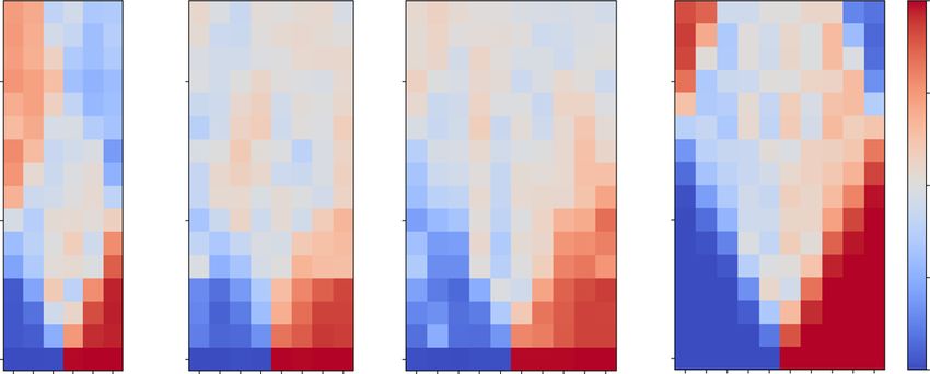
Fig. 4 Results for the connected spin correlator defined in Eq. (6). in particular, if the state is separable then we have that F Q N,
Data are computed using: a exact diagonalization, b numerical which is known as the shot noise limit in quantum metrology.78–80
trotterization, c the IBM quantum device. Data are shown for N ¼ For a general entangled state, however, the QFI is bounded by
6; hj ¼ 0 and U ¼ 0, using a symmetric trotterization, and obtained F Q N2 , and a value of F Q =N m, indicates at least m þ 1-partite
on 12 March 2019. entanglement. Note that the QFI is sensitive to the choice of the
^ and for example, if we choose O ^ /Pσ
j ^ j , the total
z
operator O,
thermalizing behaviour, resulting in the loss of this information in
local observables. With the current devices we are unfortunately
unable to distinguish these two different regimes.
Spreading of correlations—light cone
In the previous section, all the data correspond to some
combination of local average magnetizations. Here, we look at
the correlations between pairs of spatially separated spins, and
how these correlations spread. Lieb and Robinson showed that for
a local Hamiltonian, correlations can spread at most linearly and
display a light-cone causality structure.75 For instance, for tight-
binding spinless fermions, correlations spread with a speed
proportional to their maximum group velocity, v ¼ 4J.57
In Fig. 4 we compare ED, numerical trotterization and
experimental results for the connected spin correlator defined in
Eq. (6), for hj ¼ U ¼ 0. We measure correlations between the first
and the j th spin after a quench from a charge density wave initial
state. The ED results show a clear ballistic spreading of
correlations, which is also qualitatively reproduced by the
numerical trotterization and the IBM data. As with all previous
results, the agreement between the numerical and IBM results is
best at short times, but the IBM data are able to capture the point
where the correlations reach the system size. Furthermore, for this
free model, there are only significant correlations along the light-
cone and not within it, which is also approximately captured by
the experimental data. There does, however, seem to be a slightly
faster light-cone velocity, which is most evident in the shift of the
position of the peak on site 6. This indicates that there is an
effective renormalization of the Hamiltonian parameters, particu-
larly J, due to the errors in the machine.
Quantum fisher information
Finally, we consider the quantum Fisher information defined in
Eq. (7) starting from both the Néel and domain wall initial states,
shown in Fig. 5a, b, respectively. In this section, we will consider
the model of (case (i)), for which the quantum Fisher information Fig. 5 The quantum Fisher information. As computed by ED,
numerical trotterization and using the IBM quantum device for hj ¼
has two important relations to entanglement, which we outline 0 and U ¼ 0 and a symmetric trotterization. Data are compared with
below. Note that the quantum Fisher information has a more the bipartite von Neumann entanglement entropy SvN with an equal
general definition for mixed states, which reduces to our definition left/right partition, scaled by aN1 with a ¼ 32=5, see main text. a
for pure states. We do not consider the more general definition Quench from the Néel initial state. b Quench from the domain wall
since we are simulating unitary evolution from a pure quantum initial state. Data were obtained on 12 March 2019.
Published in partnership with The University of New South Wales npj Quantum Information (2019) 106A. Smith et al.
6
magnetization, then F Q ¼ 0, since our models conserve the total
magnetization.
Let us now consider the IBM results for the QFI, starting with a
quench from a Néel initial state shown in Fig. 5a. We first note that
the numerical results for the QFI (black) closely follow the bipartite
von Neumann entanglement entropy (blue). The results from the
IBM machine are also able to reproduce this behaviour quite
accurately, characterized by the linear growth with a maximum
just after Jt ¼ 1 due finite size effects. The fact that we measure
F Q =N > 1 also implies entanglement in the state on the IBM
quantum computer.
In Fig. 5b, we consider a quench from a domain wall. In this case
both the numerical and experimental simulations have the same
qualitative behaviour but are further off in absolute value, as
compared with Fig. 5a. The QFI computed on the IBM machine
once again is able to reproduce the behaviour of the von
Neummann entanglement entropy.
The entanglement entropy is generally a difficult quantity to
measure. It typically requires some form of state tomography,
which consists of a set of measurements in a number of different Fig. 6 Quantifying the accuracy of the device. a Values of MGHZ
bases that grows exponentially with system size, rendering it defined in Eq. (9) computed on the IBM device for a GHZ state on
impractical for large systems. Furthermore, even with low error three qubits. Values of MGHZ >2 cannot be explained by a classical
rates, the resulting density matrix may be unphysical.45,81 The theory of local realism, see main text. b The percentage of measured
quantum Fisher information may provide an alternative in certain states that are in the physical Hilbert space as a function of time
circumstances because it can be significantly easier to compute – after a quench from a domain
qffiffiffiffiffiffiffiffiffiffiffiffiffiffiffiffiffiffiffiffiffi
ffi wall. c Data for the computation of
for the definition that we consider we only need to measure in a the quantity U ^ 1 ðtÞUðtÞ
^ , as performed on the IBM device, after a
single basis. quench from a Néel state. Data were obtained for N ¼ 6 across four
consecutive days in 2019. Dashed lines indicate the average value
Quantifying the accuracy of the quantum computer for a randomly selected state.
While in the previous sections we showed that the current IBM
device can qualitatively reproduce physical behaviour, it is also the accuracy of the implementation of the unitary UðtÞ. ^ If the
important to develop practical quantitative measures of their implementation is non-unitary then we should expect decay with
accuracy. These measures should allow us to track the evolution of an increasing number of Trotter steps. We should also expect
the quantum computers as they are developed and improved, as
decay of this quantity if there are only unitary errors since this
well as potentially providing further insight into the various
quantity takes the form of a Loschmidt echo, which measures the
sources of error that are present.
sensitivity of the system to perturbations. It does not rely on any
Going beyond the reported gate errors, one of the simplest
^
special properties of UðtÞ, such as the presence and knowledge of
things to measure is the violation of the Mermin inequality,82
conserved quantities. It therefore provides an unbiased measure
MGHZ ¼ X^ Y^ Y^ þ Y^ X^ Y^ þ Y^ Y^ X^ X^ X^ X^ 2; (9) ^ and of the quantum
of the quality of the implementation of UðtÞ
where X;^ Y^ are the x and y Pauli-operators, and we omit the device.
consecutive site labels on the operators. This inequality should We show the computation of the identity performed on the IBM
hold for a classical theory with local realism. If we consider the machine across four consecutive days in Fig. 6c. In an ideal
GHZ state jψi ¼ p1ffiffi2 ðj """i j ###iÞ, then MGHZ ¼ 4 and this machine this quantity should be identically equal to 1 for all times.
However, with each additional Trotter step—corresponding to the
bound is maximally violated and can be used to demonstrate observed plateaux—the accuracy drops significantly. We also note
the "quantumness" of the machine. In Fig. 6a we show the values that the behaviour observed in Fig. 6b, c are very similar, and both
computed across 4 consecutive days for the first three qubits used reflect the accuracy of the simulations in the previous sections.
for the N ¼ 6 simulations. This data shows that we are consistently
able to violate the Mermin inequality.
As can be seen in the methods, the fidelities of individual gates DISCUSSION
do not necessarily reflect the accuracy of a simulation across many Probably the most striking feature of our results from the IBM
qubits. It may, therefore, make sense to consider more practical
machines is the low quantitative accuracy when compared with
measures of quality that more directly relate to the simulations we
exact numerics. Considering the limited system sizes and time
are performing. We use the physical conservation laws of the
scales that we can reach; it highlights the current limitations of
evolution to improve the accuracy of our simulations by throwing
these quantum devices. Most importantly, this shows that whilst
away measurements of unphysical states. The number of
the number of qubits is now reaching limits beyond the
measurements that are kept/thrown away can also be taken as
a quantitative measure of the effective accuracy of the machine capabilities of classical computers, the error rates and/or the
since for a perfect quantum computer we should find that all isolation of these quantum computers is not yet sufficient for
measured states are in the physical Hilbert. In Fig. 6b, we show the useful computations, at least for accurately simulating quantum
percentage of measured states that are physical for 4 consecutive dynamics. Due to the large array of possible error sources, pinning
days, showing the variation in the effective quality of the device. down the most damaging for our simulations is a difficult task,
As an unbiased measure of the quality of our and is an import practical area for future research.
qsimulation
ffiffiffiffiffiffiffiffiffiffiffiffiffiffiffiffiffiffiffiffiffiffi we Despite this unfortunate conclusion, we are still able to access a
suggest to compute the identity in the form ^I ¼ U ^ 1 ðtÞUðtÞ
^ . By range of qualitative physical behaviours demonstrating non-trivial
implementing a circuit to perform the forward and backward time simulations of quantum dynamics. We were able to compute a
evolution, the probability of returning to the initial state measures range of expectation values and two-point correlators, and
npj Quantum Information (2019) 106 Published in partnership with The University of New South WalesA. Smith et al.
7
observe behaviour associated with localization, many-body First, we discretize time, that is, we split the time evolution operator,
^ ¼ eiHt ^ ^ ¼
interactions, and the ballistic spreading of quantum correlations. UðtÞ , into a sequence of discrete operators, i.e., UðtÞ
^
UðΔtÞ ^
UðΔtÞ with fixed Δt. Each application of the discrete operator
We also observed the compensation of different energy costs due
^
UðΔtÞ is called a Trotter step. This is illustrated in Fig. 1a where we apply an
to on-site potentials and neighbouring site interactions and
increasing number of Trotter steps to reach later times.
witnessed the generation of entanglement due to unitary In our simulations we fix Δt to fix the accuracy of our approximation.
evolution through the QFI. However, since we can only implement up to 5 Trotter steps, we add
The goal of using quantum computers for dynamical simula- additional data points by varying Δt in the final Trotter step. More explictly,
tions is to be able to access systems intractable using classical consider Trotter steps M and M þ 1, we can add additional data points by
algorithms. The limitations of the current devices that we have using the evolution operator
observed in our results demonstrate the need for improved ^ ^ M^
eiHt UðΔtÞ UðδtÞ; (10)
quality of the machines and not simply adding more qubits. In this
type of simulation, the number of gates, and thus the real where δt ¼ Δt=r, where r is the number of data points we want between
execution time of the quantum circuits, grows linearly with the t ¼ MΔt and t ¼ ðM þ 1ÞΔt. Since the accuracy of the trotter decomposi-
system size and with the number of Trotter steps. This means that tion UðδtÞ is better than that of UðΔtÞ (see below), these extra data points
will have errors intermediate between that of the Mth and ðM þ 1Þth steps.
we can estimate that we would need at least an order of Second, we perform a Trotter decomposition of (trotterize) the unitary
magnitude improvement in a combination of the gate fidelities evolutions, that is, we approximately decompose the operator UðΔtÞ ^ into a
and/or T1/T2 times to get close to achieving this goal. sequence of unitaries that act on at most two neighbouring qubits. In the
One of the biggest challenges facing the field of quantum following we use either a basic or symmetric Trotter decomposition, shown
computation is how to deal with errors. Although this is primarily in Fig. 1b, c, respectively. For m Trotter steps of length Δt, the error of the
an engineering issue to increase the quality, isolation and control symmetric decomposition is of order OðmðΔtÞ3 Þ, compared with
of the devices, there is also the theoretical contribution of error OðmðΔtÞ2 Þ for the basic decomposition. Note, however, that due to the
symmetric structure, when we apply several Trotter steps we can combine
correction methods.1,83,84 A particularly promising avenue for error
several layers of gates. This means that we only need an extra two layers of
correction is to use surface codes.85,86 One big advantage of these gates compared with the basic decomposition regardless of the number of
methods is the moderately low fidelities required for them to work Trotter steps.
effectively. As the size and quality of the quantum computers Third, we must efficiently decompose these two qubit operators into the
increases, it is hoped that these error correction schemes will gates that can be directly implemented on the quantum device, which are
allow us to rapidly increase their scale, and with it their utility. In the CNOT gate and arbitrary single qubit unitaries. An efficient decomposi-
the meantime, there may also be more room for practical error tion is found in ref. 92, which we summarise below. The result is that if U ≠ 0
then B^ and C^ (defined in the figure caption) can be implemented using three
mitigation schemes, such as the one that we have used, to get the
CNOTs and with U ¼ 0 this can be reduced to only two CNOTs.
most out of NISQ devices.
While we have considered a range of correlation functions and
physical mechanisms, there is still much that can be learnt about Trotter Decomposition
the current quantum computers and how well they can simulate In this paper, we use a Trotter decomposition (commonly known as a
^
^ ¼ eiHt
quantum dynamics for condensed matter systems. In particular, trotterization) of the unitary time evolution operator UðtÞ . That is,
there are physical mechanisms beyond those that we have we want to approximate these operators by a sequence of more easily
implemented operators, namely those that act on at most two qubits.
considered here. For instance, models with gauge coupling to ^¼A
As a starting point, consider a Hamiltonian of the form H ^ þ B,^ where
dynamical gauge fields,7,39,40,53 and the physics of confine- ^ ≠ 0. Then, since these operators do not commute in general, we have
^ B
½A;
ment.87,88 In these settings there is also hope that interesting that
physics can be extracted from the short-time dynamics and thus ^ ^ ^
may be suited to the current machines. The combination of eiHt ¼ eiAt eiBt þ Oðt2 Þ; (11)
disorder and interactions, resulting in the many-body localized which can be naturally extended to Hamiltonians that are sums of more
phase, is also currently a particularly active area of than two terms. To use this fact for trotterized evolution we can use the
research.32,33,64,65 The investigation of the transition between two steps outlined in the main text. We will now go through the details of
MBL and ergodic dynamics may also benefit in the future from these steps in more detail, for the Hamiltonian Eq. (3):
quantum computation. It is notoriously difficult to study N1
X X
N1 X
N
numerically due to the requirement of large systems and/or ^ ¼ J
H σ^ xj σ ^ yj σ
^xjþ1 þ σ ^yjþ1 þ U ^zj σ^zjþ1 þ
σ hj σ^zj ; (12)
long-time simulations.89–91 j¼1 j¼1 j¼1
In conclusion, digital quantum simulation is still in its infancy which we rewrite here for convenience.
and we have shown that it requires an order of magnitude ^
First, we discretize time and split the evolution operator UðtÞ into a
^
improvement in fidelity and coherence until it will realistically product of discrete evolution operators UðΔtÞ, i.e.,
outperform classical computers, at least applied to dynamical M
^ ^
eiHt ¼ eiHΔt ; (13)
problems of interest in condensed matter physics. However, while
it is hard to predict the pace of technological progress, our results where Δt ¼ t=M and M is the number of "Trotter steps". Since the
will serve as a useful benchmark for improvements in the Hamiltonian commutes with itself, Eq. (13) is exact. To perform time
foreseeable future; and in the long run they will provide a evolution, we will typically fix Δt and increase the number of Trotter steps
snapshot of capabilities at the beginning of a new quantum M to reach later times.
simulation era. The second step is to approximate each of these discrete time operators
in a similar manner to Eq. (11). For notational simplicity, let us first define
the operators
^ j ¼ eihj σ^j Δt ; ^ ^ ^ ^
z z x x y y
Bj ¼ eiðU^σj σjþ1 Jð^σj σjþ1 þ^σj σjþ1 ÞÞΔt :
z
METHODS A (14)
Implementation: trotterized evolution
Using these operators, we can make the approximation
For our global quench protocol, we first need to prepare the initial state of ! ! !
our system. Since the IBM quantum computers are initialized in the state ^
Y Y Y
e i HΔt
¼ ^
Aj ^
Bj ^
Bj þ OððΔtÞ2 Þ; (15)
j "" i by default, both of our choices of initial states are tensor product
j j even j odd
states in the z-basis and thus can be created by applications of the Pauli X
gate. Next, we need to implement the time evolution, which proceeds by which corresponds to the schematic quantum circuit show in Fig. 1b in the
three main steps that we will briefly outline here. main text, and which we will refer to as the basic trotterization. If we wish
Published in partnership with The University of New South Wales npj Quantum Information (2019) 106A. Smith et al.
8
to evolve to time t ¼ MΔt, then we find that the error is OðΔtÞ, which is bit-flip errors can become significant and the error mitigation will be
controlled by the size of the Trotter step Δt. We can, therefore, improve the ineffective.
accuracy of the approximation by decreasing Δt, however, this must be In Fig. 6b, we show the percentage of measurements that are within the
balanced against the cost of needing more Trotter steps, as explained in physical Hilbert space, that is, the percentage of measurements that are kept.
the main text. For the first data points, we are simply measuring the initial state, which has
To improve the accuracy of our simulations, we can use better an average measurement fidelity per qubit of 95% leading to a value of
approximations to the discrete evolution operators by way of higher- approximately ð95%Þ6 70%. At long times the number of retained states
order Trotter decompositions.93 The leading error term in Eq. (11) is due to stabilises and approaches a value that corresponds to the percentage of
the non-zero commutator ½A; ^ ^
B. By compensating for this error, we can states in the total Hilbert space that are physical – in other words, the
increase the order of the leading error term. percentage probability that a randomly selected state is in the physical
The only higher-order decomposition that we will consider is the subspace. Once this number of discarded measurements is reached, the
symmetrized Trotter step. Let us again start with the simple case of errors are very large and the error mitigation is no longer effective.
^¼A
H ^ þ ^B. The symmetric decomposition would then be Bit-flips are not the only type of errors that could occur. As an example,
^ t^ ^ t^
there are also phase errors, which do not necessarily change the net
eiHt ¼ ei2A eitB ei2A þ Oðt 3 Þ: (16) magnetization. However, we note that the constrained data does typically
The error in this decomposition is of higher-order due to the symmetry have improved accuracy, and so we use the restriction to the physical
which ensures that UðtÞ ¼ UðtÞy ¼ U1 ðtÞ. This means that the even- Hilbert space for all our subsequent data.
order error terms vanish and the leading error is ðΔtÞ3 . See ref. 93 for
more details and for an iterative method for constructing higher-order Quantum Circuits
decompositions. Here, we will go over some of the details necessary to implement the
For the Hamiltonian Eq. (3) in question, let us again make some trotterized evolution operators on the IBM devices. We will only cover
definitions to simplify notation those elements of direct relevance to this paper and refer the reader to
^j ¼ eihj σ^j Δt2 ;
z
^Bj ¼ eiðU^σj σ^jþ1 Jð^σj σ^jþ1 þ^σj σ^jþ1 ÞÞΔt2 ;
z z x x y y
ref. 1 for an introduction to quantum circuits and quantum computation.
A
(17) We will first introduce the quantum gates that can be implemented on the
^ j ¼ eiðU^σj σ^jþ1 Jð^σj σ^jþ1 þ^σj σ^jþ1 ÞÞΔt ;
z z x x y y
C IBM quantum computers, and then decompose the two qubit unitary
operations that appear in our trotterized evolution operator in terms of the
then the symmetric Trotter decomposition is elementary one and two qubit gates.
! ! ! ! !
Y Y Y Y Y A quantum circuit consists of an array of quantum channels – which
^ ^j ^ ^j ^j ^ j þ OððΔtÞ3 Þ;
eiHΔt ¼ A Bj C B A represent the physical qubits—and a series of quantum gates that are
j j even j odd j even j applied to them. These quantum gates are unitary operators that can be
(18) applied to one or more of the qubits. The IBM quantum devices can
implement the CNOT gate along with an arbitrary single qubit gate,
which is shown schematically in Fig. 1c of the main text. parametrized by three phases. The cobination of these gates forms a
universal set that is, any N qubit gate can be implemented using a
Measurement combination of these gates, and in principle an arbitrary quantum
When making a measurement we will find the system in one of the many- computation can be performed.
body states jλi in this basis, e.g., j "## i or j #"# i. By performing There is a collection of single particle gates that are useful for writing
multiple runs and measurements, we can approximate the probability of quantum circuits. We write down a list of the most frequently used gates
measuring each of the many-body states, that is, we can extract jαλ j2 , and how they are implemented on the IBM machines. Consider the
where αλ is the probability amplitude for the state jλi. These probabilities computational basis to be the tensor product of single qubit states in the
can then be used to construct the observables. To be more concrete, z-basis, i.e., fj "i; j #ig. All matrix forms of the gates are given in this basis
consider the expectation value of the operator σ ^ zj on site j. This is and all measurements are made in this z-basis. It is important to note that
computed as follows, gate multiplication reads left to right, whereas matrix multiplication is right
X X to left, i.e. .
hψðtÞjσ^zj jψðtÞi ¼ jαλ j2 jαλ0 j2 ; (19)
0
Firstly, we have the Pauli matrices, which in the standard quantum
λ:j¼" λ :j¼#
information notation are
where the sums are over all states with the j th spin up or down respectively,
and jαλ j2 is the proportion of measurements for which we found the state λ.
In all the following experiments we will use 8192 measurements per data
point, which means that the statistical error for these local correlators is ð20Þ
0:01, which is too small to be included in our figures.
Error mitigation: physical Hilbert space Secondly, we have the Hadamard and the S and T phase gates,
As we noted in the previous section, due to the presence of conserved
quantities in the Hamiltonian evolution, the Hilbert space of states splits
into those that are physically allowed by the evolution and those that
are not. In particular,
P the models we consider have conserved net ð21Þ
magnetization Sz ¼ j σ^zj . This fact turns out to be advantageous, and
allows us to perform rudimentary error mitigation – a term that we use
to distinguish it from scalable error correction methods, since in this
case we deal only with the lowest order errors. The idea is to simply And finally, we have the X; Y and Z rotation gates,
disregard any measurements for states outside of the physical Hilbert
space. Let use present a simplified argument for why this might be a
good thing to do, where we will first assume that only bit-flips
can occur.
A single bit-flip in the course of the evolution will take us outside of
ð22Þ
the Hilbert space, and let us denote the probability of this happening as
Δ. However, the lowest order of errors within the physical Hilbert space
is Δ2 , i.e., we need at least two bit-flip errors to get back to the same
total magnetization. Hence, by discarding counts outside of the physical
Hilbert space we reduce the leading order error to Δ2 . If the probability,
Δ, is sufficiently small, then we can rely on these perturbative which correspond to rotations of the qubit around the x; y and z axes
arguments. However, if the error rate is large enough, then multiple respectively. All single qubit gates can be written as a product of these
npj Quantum Information (2019) 106 Published in partnership with The University of New South WalesA. Smith et al.
9
rotation gates, up to a phase. This phase is global and is not measurable unitary operators. We, therefore, want to find a way to write a general two
and can therefore be omitted. In the IBM machine, all single qubit gates qubit unitary in terms of the CNOT gate and single qubit gates that can be
can be directly implemented using applied directly on the IBM devices. The optimal decomposition is found in
ref. 92. We briefly review the main results of this paper that are of direct
relevance to us.
ð23Þ The optimal decomposition uses the fact that a general matrix in Uð4Þ
can be decomposed as U ¼ ðA1 A2 Þ Nðα; β; γÞ ðA3 A4 Þ,94 where
Nðα; β; γÞ ¼ exp½i ðασx σx þ βσy σ y þ γσ z σ z Þ: (28)
For slightly less general gates the IBM computer implements either
U2 ðϕ; λÞ ¼ U3 ð0; ϕ; λÞ or U1 ðλÞ ¼ U3 ð0; 0; λÞ, which use fewer physical As a quantum circuit, this can be written as
operations and shorter real time. Before running the circuits, we can
combine all strings of single qubit gates into a single one of these three
single qubit gates, using the functions available in qiskit.42
The most important two qubit gate for our purposes is the CNOT gate ð29Þ
This operator Nðα; β; γÞ is of direct interest to us for quantum dynamics
ð24Þ
since it is already of the form required for our Trotter decomposition. This
gate can be constructed using a minimum of three CNOTs. The optimal
decomposition for Nðα; β; γÞ is given by the quantum circuit
This gate flips the second qubit depending on the state of the first. This
gate allows the two qubits to become entangled, and combined with
general single qubit gates forms a set capable of universal quantum ð30Þ
computation, see ref. 1 for a proof. The CNOT is the only multi-qubit gate
currently that can be directly implemented on the IBM quantum machines.
Also of interest to us is the reversed CNOT gate
where θ ¼ π2 2γ; ϕ ¼ 2α π2, and λ ¼ π2 2β. Note that in ref. 92 they use
a different sign convention for the rotation gates. Despite the apparent
asymmetry of the decomposition, this sequence of gates is symmetric with
ð25Þ respect to swapping the two qubits.
For certain cases of our Hamiltonian, namely when U ¼ 0, the Nðα; β; γÞ
gate is more general than we need. By restricting ourselves to Nðα; 0; γÞ
(plus single qubit basis changes) we can reduce the number of CNOTs
where we differentiate the reversed CNOT from the CNOT because of the required to two. This gives us access to matrices of the form
directionality of the IBM machines, i.e., only CNOTs in a given direction can Nðα; 0; γÞ ¼ exp½iðασx σ x þ γσ z σ z Þ: (31)
be implemented along the qubit connections. If a CNOT is applied
(programmatically) in the wrong directly, the above transformation using We can proceed with the help of the so-called Magic Matrix92,94
Hadamard gates will be applied by qiskit implicitly. Since the single qubit
gate fidelities are an order of magnitude better than that of the CNOTs this
transformation is not costly, and these additional gates will often be ð32Þ
incorporated into other strings of single qubit gates.
Using this matrix we find My Nðα; 0; γÞM ¼ eiγσ
z z
Change of basis eiασ , which in turn
eiασ ÞMy , since M is unitary. As a
z z
When we make a measurement on the quantum machine it is with respect implies that Nðα; 0; γÞ ¼ Mðeiγσ
to a given basis, which we take to be the z-basis. However, we may choose quantum circuit this can be written as
to change the basis for several reasons such as: to measure different
operators, to prepare an initial state, or to apply a gate which is more
efficiently implemented in a different basis.
We will consider only local changes of basis, i.e. a change of basis for the ð33Þ
individual qubits. While a general local change of basis can be
implemented using the general single qubit gates above, the most
frequently used will be those that change from the Z basis to the X or
Y basis. This gate can be further simplified by noting that a product of single qubit
To change to the X basis, we use the Hadamard gate, H. This implements gates is another single qubit gate. Furthermore, ½S; Rz ðθÞ ¼ 0, and
the transformation HRz ðθÞH ¼ Rx ðθÞ which gives
Z ! X; X ! Z; Y ! Y: (26)
Note that this mapping is its own inverse, which is a result of the ð34Þ
Hadamard gate being both unitary and Hermitian.
To change to the Y basis, we use a combination of the Hadamard and S
gates. We can implement the basis change with the combination HSH, where we have arbitrarily flipped the circuit with respect to the two qubits.
which maps
Z ! Y; Y ! Z; X ! X: (27) Choosing the best qubits
Note that this combination of gates is not its own inverse but instead is In all our numerics we used between 6 and 10 of the qubits of the IBM
HSy H. machines, which is only a subset of the available 20 qubits. Hence, we
wish to find the best such subset so that we get the most accurate
results from the machine. We do this by using a simple iterative
Two qubit gates algorithm, which we will outline here. We note that "best" is a matter of
The Trotter decomposition allows us to write the general unitary time definition involving the balance of many different parameters. We define
evolution operator approximately as a product of single and two qubit best to mean the set of qubits that has the lowest average CNOT errors.
Published in partnership with The University of New South Wales npj Quantum Information (2019) 106You can also read