NEEDLES IN HAYSTACKS: ON CLASSIFYING TINY OBJECTS IN LARGE IMAGES
←
→
Page content transcription
If your browser does not render page correctly, please read the page content below
N EEDLES IN H AYSTACKS :
                                        O N C LASSIFYING T INY O BJECTS IN L ARGE I MAGES
                                            Nick Pawlowski1∗            Suvrat Bhooshan2         Nicolas Ballas2
                                            Francesco Ciompi3             Ben Glocker1          Michal Drozdzal2
                                         1
                                             Biomedical Image Analysis Group, Imperial College London, UK
                                         2
                                             Facebook AI Research
                                         3
                                             Department of Pathology, Radboud University Medical Center, Nijmegen, Netherlands
                                         n.pawlowski16@imperial.ac.uk
arXiv:1908.06037v2 [cs.CV] 6 Jan 2020

                                                                                          A BSTRACT

                                                      In some important computer vision domains, such as medical or hyperspectral
                                                      imaging, we care about the classification of tiny objects in large images. However,
                                                      most Convolutional Neural Networks (CNNs) for image classification were de-
                                                      veloped using biased datasets that contain large objects, in mostly central image
                                                      positions. To assess whether classical CNN architectures work well for tiny object
                                                      classification we build a comprehensive testbed containing two datasets: one de-
                                                      rived from MNIST digits and one from histopathology images. This testbed allows
                                                      controlled experiments to stress-test CNN architectures with a broad spectrum of
                                                      signal-to-noise ratios. Our observations indicate that: (1) There exists a limit to
                                                      signal-to-noise below which CNNs fail to generalize and that this limit is affected
                                                      by dataset size — more data leading to better performances; however, the amount
                                                      of training data required for the model to generalize scales rapidly with the inverse
                                                      of the object-to-image ratio (2) in general, higher capacity models exhibit better
                                                      generalization; (3) when knowing the approximate object sizes, adapting receptive
                                                      field is beneficial; and (4) for very small signal-to-noise ratio the choice of global
                                                      pooling operation affects optimization, whereas for relatively large signal-to-noise
                                                      values, all tested global pooling operations exhibit similar performance.

                                        1        I NTRODUCTION

                                        Convolutional Neural Networks (CNNs) are the current state-of-the-art approach for image classifica-
                                        tion (Krizhevsky et al., 2012; Simonyan & Zisserman, 2014; He et al., 2015; Huang et al., 2017). The
                                        goal of image classification is to assign an image-level label to an image. Typically, it is assumed
                                        that an object (or concept) that correlates with the label is clearly visible and occupies a significant
                                        portion of the image (Lecun et al., 1998; Krizhevsky, 2009; Deng et al., 2009). Yet, in a variety of
                                        real-life applications, such as medical image or hyperspectral image analysis, only a small portion of
                                        the input correlates with the label, resulting in low signal-to-noise ratio. We define this input image
                                        signal-to-noise ratio as Object to Image (O2I) ratio. The O2I ratio range for three real-life datasets is
                                        depicted in Figure 1. As can be seen, there exists a distribution shift between standard classification
                                        benchmarks and domain specific datasets. For instance, in the ImageNet dataset (Deng et al., 2009)
                                        objects fill at least 1% of the entire image, while in histopathology slices (Ehteshami Bejnordi et al.,
                                        2017) cancer cells can occupy as little as 10−6 % of the whole image.
                                        Recent works have studied CNNs under different noise scenarios, either by performing random
                                        input-to-label experiments (Zhang et al., 2017; Arpit et al., 2017) or by directly working with noisy
                                        annotations (Mahajan et al., 2018; Jiang et al., 2017; Han et al., 2018). While, it has been shown
                                        that large amounts of label-corruption noise hinders the CNNs generalization (Zhang et al., 2017;
                                        Arpit et al., 2017), it has been further demonstrated that CNNs can mitigate this label-corruption
                                        noise by increasing the size of training data (Mahajan et al., 2018), tuning the optimizer hyperpa-
                                        rameters (Jastrz˛ebski et al., 2017) or weighting input training samples (Jiang et al., 2017; Han et al.,
                                             ∗
                                                 Work done as part of an internship at Facebook AI Research.

                                                                                                 1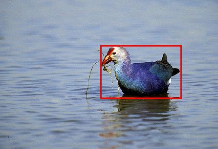
CAMELYON17 MiniMIAS
10−6 10−5 10−4 10−3 10−2 10−1 100 101 102
ImageNet
ImageNet MiniMIAS CAMELYON17
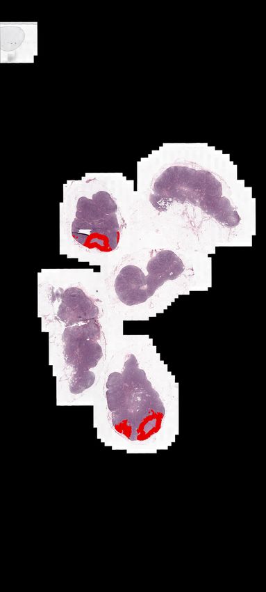
Figure 1: Range of Object to Image (O2I) ratios [%] for two medical imaging datasets (CAME-
LYON17 (Ehteshami Bejnordi et al., 2017) and MiniMIAS (Suckling, 1994)) as well as one standard
computer vision classification dataset (ImageNet (Deng et al., 2009)). The ratio is defined as
Aobject
O2I = Aimage , where Aobject and Aimage denote the area of the object and the image, respectively.
Together with O2I range, we display examples of images jointly with the object area Aobject (in red).
2018). However, all these works focus on input-to-label corruption and do not consider the case of
noiseless input-to-label assignments with low and very low O2I ratios.
In this paper, we build a novel testbed allowing us to specifically study the performance of CNNs
when applied to tiny object classification and to investigate the interplay between input signal-to-noise
ratio and model generalization. We create two synthetic datasets inspired by the children’s puzzle
book Where’s Wally? (Handford, 1987). The first dataset is derived from MNIST digits and allows us
to produce a relatively large number of datapoints with explicit control of the O2I ratio. The second
dataset is extracted from histopathology imaging (Ehteshami Bejnordi et al., 2017) where we crop
images around lesions and obtain small number of datapoints with an approximate control of the O2I
ratio. To the best of our knowledge these datasets are the first ones designed to explicitly stress-test
the behaviour of the CNNs in the low input image signal-to-noise ratio.
We develop a classification framework, based on CNNs, and analyze the effects of different factors
affecting the model optimization and generalization. Throughout an empirical evaluation, we make
the following observations:
– Models can be trained in low O2I regime without using any pixel-level annotations and
generalize if we leverage enough training data. However, the amount of training data
required for the model to generalize scales rapidly with the inverse of the O2I ratio. When
considering datasets with fixed size, we observe an O2I ratio limit in which all tested
scenarios fail to exceed random performance.
– We empirically observe that higher capacity models show better generalization. We hy-
pothesize that high capacity models learn the input noise structure and, as result, achieve
satisfactory generalization.
– We confirm the importance of model inductive bias — in particular, the model’s receptive
field size. Our results suggest that different pooling operations exhibit similar performance,
for larger O2I ratios; however, for very small O2I ratios, the type of pooling operation
affects the optimization ease, with max-pooling leading to fastest convergence.
The code of our testbed will be publicly available at: https://anonymous.url allowing to
reproduce all data and results; we hope this work can serve as a valuable resource facilitating further
research into the understudied problem of low signal-to-noise classification scenarios.
2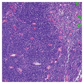
(a) O2I ratio = 0.3%    (b) O2I ratio = 0.075%       (c) O2I ratio ∈ [1 − 10]%   (d) O2I ratio ∈ [0.1 − 1]%

Figure 2: Example images from our nMNIST (a, b) and nCAMELYON (c, d) datasets with different
O2I ratios. The object of interest is marked by red (nMNIST) or green outlines (nCAMELYON).

2      T ESTBED FOR LOW SIGNAL - TO - NOISE CLASSIFICATION SCENARIOS

2.1     DATASETS : I S THERE A WALLY IN AN IMAGE ?

To study the optimization and generalization properties of CNNs, we build two datasets: one derived
from the MNIST (Lecun et al., 1998) dataset and another one produced by cropping large resolution
images from the CAMELYON dataset (Ehteshami Bejnordi et al., 2017). Each dataset allows to
evaluate the behaviour of a CNN-based binary classifier when altering different data-related factors
of variation such as dataset size, object size, image resolution and class balance. In this subsection,
we describe the data generation process.
Digits: needle MNIST (nMNIST). Inspired by the cluttered MNIST dataset (Ba et al., 2015),
we introduce a scaled up, large resolution cluttered MNIST dataset, suitable for binary image
classification. In this dataset, images are obtained by randomly placing a varying number of MNIST
digits on a large resolution image canvas. We keep the original 28 × 28 pixels digit resolution and
control the O2I ratio by increasing the resolution of the canvas 1 . As result, we obtain the following
O2I ratios {19.1, 4.8, 1.2, 0.3, and 0.075}% that correspond to the following canvas resolutions
64 × 64, 128 × 128, 256 × 256, 512 × 512, and 1024 × 1024 pixels, respectively. As object of interest,
we select digit 3. All positive images contain exactly one instance of the digit 3 randomly placed
within the image canvas, while negative instances do not contain any instance. We also include
distractors (clutter digits): any MNIST digit image sampled with replacement from a set of labels
{0, 1, 2, 4, 5, 6, 7, 8, 9}. We maintain approximately constant clutter density over different O2I ratios.
Thus, the following O2I ratios {19.1, 4.8, 1.2, 0.3, and 0.075}% correspond to 2, 5, 25, 100, and 400
clutter objects, respectively. For each value of O2I ratio, we obtain 11276, 1972, 4040 of training,
validation and test images2 . Fig. 2 depicts example images for different O2I ratios. We refer the
interested reader to the supplementary material for details on image generation process as well as
additional dataset visualizations.
Histopathology: needle CAMELYON (nCAMELYON). The CAMELYON (Ehteshami Bejnordi
et al., 2017) dataset contains gigapixel hystopathology images with pixel-level lesion annotations from
5 different acquisition sites. We use the pixel-wise annotations to extract crops with controlled O2I
ratios. Namely, we generate datasets for O2I ratios in the range of (100−50)%, (50−10)%, (10−1)%,
and (1 − 0.1)%, and we crop different image resolutions with the size of 128 × 128, 256 × 256,
and 512 × 512 pixels. This results in training sets of about 20 − 235 unique lesions per dataset
configuration (see supplementary for a detailed list of dataset sizes). More precisely, positive examples
are created by taking 50 random crops from every contiguous lesion annotation and rejecting the
crop if the O2I ratio does not fall within the desired range. Negative images are taken by randomly
cropping healthy images and filtering image crops that mostly contain background. We ensure the
class balance by sampling an equal amount of positive and negative crops. Once the crops were
extracted, no pixel-wise information is used during training. Figure 2 shows examples of extracted
   1
     Alternatively, we could fix canvas image resolution and downscale MNIST digits; however, downscaling
might reduce the object quality.
   2
     We obtain those numbers by using the original MNIST data, we use every digit 3 only once to generate
positive images and we balance the dataset with negative images. See supplementary material for class
imbalanced data scenarios.

                                                     3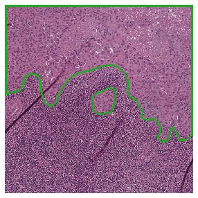
Figure 3: Pipeline. Our pipeline is built of three com-
ponents: (1) a CNN extracting topological embedding,            Figure 4: Image-level annotations.
(2) a global pooling operation and (3) a binary classifier.    Test set accuracy vs. O2I ratio for
See text for details.                                           best models, see text for details.
images used in the nCAMELYON dataset experiments. We refer to the supplementary for more detail
about the data extraction process, the resulting dataset sizes and more visualizations.

2.2   M ODELS

Our classification pipelines follow BagNets (Brendel & Bethge, 2019) backbone, which allows us to
explicitly control for the network receptive field size. Figure 3 shows a schematic of our approach.
As can be seen, the pipelines are built of three components: (1) topological embedding extractor in
which we can control for embedding receptive field, (2) global pooling operation that converts the
topological embedding into a global embedding, and (3) a binary classifier that receives the global
embedding and outputs binary classification probabilities. By varying the embedding extractor and
the pooling operation, we test a set of 48 different architectures.
Topological embedding extractor. The extractor takes as input an image I of size [wimg × himg ×
cimg ] and outputs a topological embedding Et of shape [wenc × henc × cenc ], where w. , h. , and c.
represent width, height and number of channels. Due to the relatively large image sizes, we train
the pipeline with small batch sizes and, thus, we replace BagNet-used BatchNorm operation (Ioffe
& Szegedy, 2015) with Instance Normalization (Ulyanov et al., 2016). In our experiments, we test
12 different extractor architectures obtained by adapting embedding extractor receptive field and
capacity. For model details, please refer to section B.2 in the supplementary material.
Global pooling operation. Global pooling operation takes as an input topological embedding Et of
shape [wenc × henc × cenc ] and outputs global image embedding EI of shape [1 × 1 × cenc ]. In the
paper, we experiment with four different pooling operations, namely: max, logsumexp, average, and
soft attention. In our experiments, we follow the soft attention formulation of (Ilse et al., 2018). The
details about global pooling operations can be found in the supplementary material.

3     E XPERIMENTAL RESULTS

In this section, we experimentally test how CNNs’ optimization and generalization scale with low
and very low O2I ratios. First, we provide details about our experimental setup and then we design
experiments to provide empirical evidence to the following questions: (1) Image-level annotations:
Is it possible to train classification systems that generalize well in low and very low O2I scenarios?
(2) O2I limit vs. dataset size: Is there an O2I ratio limit below which the CNNs will experience
generalization difficulties? Does this O2I limit depend on the dataset size? (3) O2I limit vs. model
capacity: Do higher capacity models generalize better? (4) Inductive bias - receptive field: Is
adjusting receptive field size to match (or exceed) the expected object size beneficial? (5) Global
pooling operations: Does the choice of global pooling operation affect model generalization? Finally,
we inquire about the optimization ease of the models trained on data with very low O2I ratios.
In all our experiments, we used RMSProp (Tieleman & Hinton, 2012) with a learning rate of
η = 5 · 10−5 and decayed the learning rate multiplying it by 0.1 at 80, 120 and 160 epochs 3 . All
   3
     Before committing to a single optimization scheme, we evaluated a variety of optimizers (Adam, RMSprop
and SGD with momentum), learning rates (η ∈ {1, 2, 3, 5, 7, 10} · 10−5 ), and 3 learning rate schedules.

                                                    4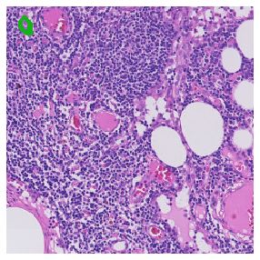
(a) nMNIST                           (b) nMNIST                       (c) nCAMELYON

Figure 5: Testing the O2I limit. Subfigure (a) depicts the test set performance as a function of
training dataset size for the nMNIST dataset, while subfigures (b) and (c) show the test set performance
as a function of model capacity for the nMNIST dataset and the nCAMELYON dataset, respectively.

            (a) nMNIST                                            (b) nMNIST

Figure 6: Testing the O2I limit. (a) mean validation set accuracy heatmap for max pooling operation,
and (b) minimum required training set size to achieve the noted validation accuracy. We test training
set sizes ∈ {1400, 2819, 5638, 7500, 11276, 22552} and report the minimum amount of training
examples that achieve a specific validation performance pooling over different network capacities.

models were trained with cross entropy loss for a maximum of 200 epochs. We used an effective batch
size of 32. If the batch did not fit into memory we used smaller batches with gradient accumulation.
To ensure robustness of our conclusions, we run every experiment with six different random seeds and
report the mean and standard deviation. Throughout the training we monitored validation accuracy,
and reported test set results for the model that achieved best validation set performance.

3.1   R ESULTS

In this subsection, we present and discuss the main results of our analysis. Unless stated otherwise,
the capacity of the ResNet-50 network is about 2.3 · 107 parameters. Additional results and analysis
are presented in the supplementary material.
Image-level annotations: For this experiment, we vary the O2I ratio on nMNIST and nCAMELYON
to test its influence on the generalization of the network. Figure 4 depicts the results for the best
configuration according to the validation performance: we use max-pooling and receptive field
sizes of 33 × 33 and 9 × 9 pixels for the nMNIST and nCAMELYON datasets, respectively. For
the nMNIST dataset, the plot represents the mean over 6 random seeds together with the standard
deviation; while for the nCAMELYON dataset we report an average over both the 6 seeds and the
crop sizes. We find that the tested CNNs achieve reasonable test set accuracies for the O2I ratios
larger than 0.3% for the nMNIST datset and the O2I ratios above 1% for the histopathology dataset.
For both datasets, smaller O2I ratios lead to poor or even random test set accuracies.
O2I limit vs. dataset size: We test the influence of the training set size on model generalization for
the nMNIST data, to understand the CNNs’ generalization problems for very small O2I ratios. We

                                                   5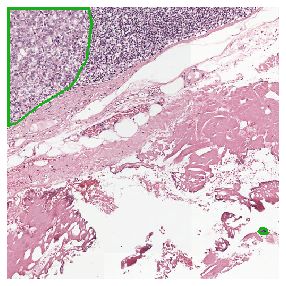
(a) nMNIST                             (a) nMNIST                             (a) nMNIST

       (b) nCAMELYON                          (b) nCAMELYON                             (b) nMNIST
Figure 7: Inductive bias: for          Figure 8: Global pooling op-    Figure 9: nMNIST optimiza-
(a) the nMNIST dataset and             erations: for (a) the nMNIST    tion: (a) number of training
(b) the nCAMELYON dataset.             dataset and (b) the nCAME-      epochs needed to fit the 11k
We report only runs that fit the       LYON datset. We report only     training data and (b) the num-
training data. Otherwise we            runs that fit the training data.ber of successful runs. The
report random accuracy and             Otherwise we report random      textured bars indicate that the
depict it with a texture on the        accuracy and depict it with a   model did not fit the training
bars.                                  texture on the bars.            data for all random seeds.
tested six different dataset sizes (1400, 2819, 5638, 7500, 11276, 22552) 4 . Fig. 5a depicts the results
for max-pooling and a receptive field of 33 × 33 pixels. We observe that larger datasets yield better
generalization and this increment is more pronounced for small O2I ratios. For further insights, we
plot a heatmap representing the mean validation set results 5 for all considered 02Is and training set
sizes (Fig. 6a) as well as the minimum number of training examples to achieve a validation accuracy
of 70% and 85% (Fig. 6b). We observe that in order to achieve good classification generalization the
required training set size rapidly increases with the decrease of the O2I ratio.
O2I limit vs. capacity: In this experiment, we train networks with different capacities — by
uniformly scaling the initial number of filters in convolutional kernels by [ 14 , 12 , 1, and 2]6 . We show
the CNNs test set performances as a function of the O2I ratio and the network capacity in Figures 5b
and 5c for the nMNIST (with 11k training points) and nCAMELYON data, respectively. On nMNIST,
we observe a clear trend, where the model test set performance increases with capacity and this boost
is larger for smaller O2Is. We hypothesize, that this generalization improvement is due to the model
ability to learn-to-ignore the input data noise; with smaller O2I there is more noise to ignore and,
   4
     We allow to reuse each digit 3 for larger training sets and select a subset for smaller training sets.
   5
     More precisely, we plot the mean of all pipeline configurations that surpassed 70% training accuracy.
   6
     We chose the maximum scaling factor so that the largest resolution images still fit in available GPU memory.
For images with O2I ratio of 0.07, the available GPU memory prevents testing networks with higher capacity.

                                                       6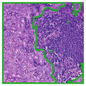
thus, higher network capacity is required to solve the task. However, for the nCAMELYON dataset,
this trend is not so pronounced and we attribute this to the limited dataset size (more precisely to the
small number of unique lesions). These results suggest that collecting a very large histopathology
dataset might enable training of CNN models using only image level annotations.
Inductive bias - receptive field: We report the test accuracy as a function of the O2I ratio and the
receptive field size for nMINIST in Figure 7a and for nCAMELYON in Figure 7b. Both plots depict
results for the global max pooling operation. For nMNIST, we observe that a receptive field that is
bigger than the area occupied by one single digit leads to best performances; for example, receptive
fields of 33 × 33 and 177 × 177 pixels clearly outperform the smallest tested receptive field of 9 × 9
pixels. However, for the nCAMELYON dataset we observe that the smallest receptive field actually
performs best. This suggests that most of the class-relevant information is contained in the texture and
that higher receptive fields pick up more spurious correlations, because the capacity of the networks
is constant.
Global pooling operations: In this experiment, we compare the performance of four different
pooling approaches. We present the relation between test accuracy and pooling function for different
O2I ratios with a receptive field of 33 × 33 pixels for nMNIST in Figure 8a and 9 × 9 pixels for
nCAMELYON in Figure 8b. On the one hand, for the nMNIST dataset, we observe that for the
relatively large O2I ratios, all pooling operations reach similar performance; however, for smaller
O2Is we see that max-pooling is the best choice. We hypothesize that the global max pooling
operation is best suited to remove nMNIST-type of structured input noise. On the other hand, when
using the histopathology dataset, for the smallest O2I mean and soft attention poolings reach best
performances; however, these outcomes might be affected by the relatively small nCAMELYON
dataset used for training.
Optimization: In our large scale nMNIST experiments (when using ≈ 11k datapoints), we observed
that some configurations have problems fitting the training data 7 . In some runs, after significant
efforts put into CNNs hyperparamenter selection, the training accuracy was close to random. To
investigate this issue further, we followed the setup of randomized experiments from (Zhang et al.,
2017; Arpit et al., 2017) and we substituted the nMNIST datapoints with samples from an isotropic
Gaussian distribution. On the one hand, we observed that all the tested setups of our pipeline were able
to memorize the Gaussian samples, while, on the other hand, most setups were failing to memorize
the same-size, nMNIST datataset for small and very small O2I ratios. We argue that the nMNIST
structured noise and its compositionality may be a “harder” type of noise for the CNNs than Gaussian
isotropic noise. To provide further experimental evidence, we depict average time-to-fit the training
data (in epochs) in Fig. 9a as well as number of successful optimizations in Fig. 9b for different
O2I ratios and pooling methods8 . We observe that the optimization gets progressively harder with
decreasing O2I ratio (with max pooling being the most robust). Moreover, we note that the results are
consistent across different random seeds, where all runs either succeed or fail to converge.

4       R ELATED W ORK

4.1       T INY O BJECT C LASSIFICATION

Reasoning about tiny objects is of high interest in many computer vision areas, such as medical
imaging (Ehteshami Bejnordi et al., 2017; Aresta et al., 2018; Setio et al., 2017; Suckling, 1994;
Sudre et al., 2018) and remote sensing (Xia et al., 2018; Pang et al., 2019). To overcome the low
signal-to-noise ratio, most approaches rely on manual dataset “curation” and collect additional
pixel-level annotations such as landmark positions (Borovec et al., 2018), bounding boxes (Wei
et al., 2019; Resta et al., 2011) or segmentation maps (Ehteshami Bejnordi et al., 2017). This
additional annotation allows to transform the original needle-in-a-haystack problem into a less noisy
but imbalanced classification problem (Wei et al., 2019; Lee & Paeng, 2018; Bándi et al., 2019).
However, collecting pixel level annotations has a significant cost and might require expert knowledge,
and as such, is a bottleneck in the data collection process.

    7
        We did not observe optimization problems for small dataset sizes of the nMNIST nor for nCAMELYON.
    8
        We define an optimization to be successful if it the training set accuracy surpassed 99%.

                                                      7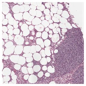
Other approaches leverage the fact that task-relevant information is often not uniformly distributed
across input data, e.g. by using attention mechanisms to process very high-dimensional inputs (Mnih
et al., 2014; Ba et al., 2015; Almahairi et al., 2016; Katharopoulos & Fleuret, 2019). However, those
approaches are mainly motivated from a computational perspective trying to reduce the computational
footprint at inference time.
Some recent research has also studied attention based approaches both in the context of multi-instance
learning (Ilse et al., 2018) and histopathology image classification (Tomita et al., 2018). However,
neither of the works report the exact O2I ratio used in the experiments.

4.2       G ENERALIZATION OF CNN S

In this subsection, we briefly highlight the dimensions of optimization and generalization of CNN
that are handy in low O2I classification scenarios.
Model capacity. For fixed training accuracy, over-parametrized CNNs tend to generalize better (No-
vak et al., 2018). In addition, when properly regularized and given a fixed size dataset, higher capacity
models tend to provide better performance (He et al., 2016; Huang et al., 2017). However, finding
proper regularization is not trivial (Goodfellow et al., 2016).
Dataset size. CNN performance improves logarithmically with dataset size (Sun et al., 2017).
Moreover, in order to fully exploit the data benefit, the model capacity should scale jointly with the
dataset size (Mahajan et al., 2018; Sun et al., 2017).
Model inductive biases. Inductive biases limit the space of possible solutions that a neural network
can learn (Goodfellow et al., 2016). Incorporating these biases is an effective way to include data
(or domain) specific knowledge in the model. Perhaps the most successful inductive bias is the use
of convolutions in CNNs (LeCun & Bengio, 1998). Different CNN architectures (e. g. altering
network connectivity) also lead to improved model performance (He et al., 2016; Huang et al., 2017).
Additionally, it has been shown on the ImageNet dataset that CNN accuracy scales logarithmically
with the size of the receptive field (Brendel & Bethge, 2019).

5       D ISCUSSION AND C ONCLUSIONS
Although low input image signal-to-noise scenarios have been extensively studied in signal processing
field (e.g. in tasks such as image reconstruction), less attention has been devoted to low signal-to-
noise classification scenarios. Thus, in this paper we identified an unexplored machine learning
problem, namely image classification in low and very low signal-to-noise ratios. In order to study such
scenarios, we built two datasets that allowed us to perform controlled experiments by manipulating the
input image signal-to-noise ratio and highlighted that CNNs struggle to show good generalization for
low and very low signal-to-noise ratios even for a relatively elementary MNIST-based dataset. Finally,
we ran a series of controlled experiments9 that explore both a variety of CNNs’ architectural choices
and the importance of training data scale for the low and very low signal-to-noise classification. One
of our main observation was that properly designed CNNs can be trained in low O2I regime without
using any pixel-level annotations and generalize if we leverage enough training data; however, the
amount of training data required for the model to generalize scales rapidly with the inverse of the O2I
ratio. Thus, with our paper (and the code release) we invite the community to work on data-efficient
solutions to low and very low signal-to-noise classification.
Our experimental study exhibits limitations: First, due to the lack of large scale datasets that allow
for explicit control of the input signal-to-noise ratios, we were forced to use the synthetically built
nMNIST dataset for most of our analysis. As a real life dataset, we used crops from the histopathology
CAMELYON dataset; however, due to relatively a small number of unique lesions we were unable
to scale the histopathology experiments to the extent as the nMNIST experiments, and, as result,
some conclusions might be affected by the limited dataset size. Other large scale computer vision
datasets like MS COCO (Lin et al., 2014) exhibit correlations of the object of interest with the image
background. For MS COCO, the smallest O2I ratios are for the object category "sports ball" which
on average occupies between 0.3% and 0.4% of an image and its presence tends to be correlated
with the image background (e. g. presence of sports fields and players). However, future research
    9
        We ran more than 750 experiments each with 6 different seeds.

                                                        8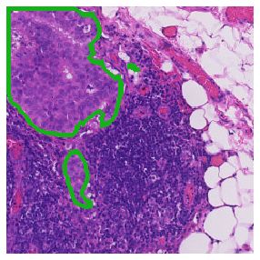
could examine a setup in which negative images contain objects of the categories "person" and
"baseball bat" and positive images also contain "sports ball". Second, all the tested models improve
the generalization with larger dataset sizes; however, scaling datasets such as CAMELYON to tens of
thousands of samples might be prohibitively expensive. Instead, further research should be devoted
to developing computationally-scalable, data-efficient inductive biases that can handle very low
signal-to-noise ratios with limited dataset sizes. Future work, could explore the knowledge of the low
O2I ratio and therefore sparse signal as an inductive bias. Finally, we studied low signal-to-noise
scenarios only for binary classification scenarios 10 ; further investigation should be devoted to multi-
class problems. We hope that this study will stimulate the research in image classification for low
signal-to-noise input scenarios.

R EFERENCES
Amjad Almahairi, Nicolas Ballas, Tim Cooijmans, Yin Zheng, Hugo Larochelle, and Aaron Courville.
 Dynamic capacity networks. In International Conference on Machine Learning, pp. 2549–2558,
 2016.
Guilherme Aresta, Teresa Araújo, Scotty Kwok, Sai Saketh Chennamsetty, Mohammed Safwan K. P.,
  Alex Varghese, Bahram Marami, Marcel Prastawa, Monica Chan, Michael J. Donovan, Gerardo
  Fernandez, Jack Zeineh, Matthias Kohl, Christoph Walz, Florian Ludwig, Stefan Braunewell,
  Maximilian Baust, Quoc Dang Vu, Minh Nguyen Nhat To, Eal Kim, Jin Tae Kwak, Sameh Galal,
  Veronica Sanchez-Freire, Nadia Brancati, Maria Frucci, Daniel Riccio, Yaqi Wang, Lingling Sun,
  Kaiqiang Ma, Jiannan Fang, Ismaël Koné, Lahsen Boulmane, Aurélio Campilho, Catarina Eloy,
  António Polónia, and Paulo Aguiar. BACH: grand challenge on breast cancer histology images.
  CoRR, abs/1808.04277, 2018. URL http://arxiv.org/abs/1808.04277.
Devansh Arpit, Stanislaw K. Jastrzebski, Nicolas Ballas, David Krueger, Emmanuel Bengio, Maxin-
  der S. Kanwal, Tegan Maharaj, Asja Fischer, Aaron C. Courville, Yoshua Bengio, and Simon
  Lacoste-Julien. A closer look at memorization in deep networks. In Proceedings of the 34th Inter-
  national Conference on Machine Learning, ICML 2017, Sydney, NSW, Australia, 6-11 August 2017,
  pp. 233–242, 2017. URL http://proceedings.mlr.press/v70/arpit17a.html.
Jimmy Ba, Volodymyr Mnih, and Koray Kavukcuoglu. Multiple object recognition with visual
  attention. In ICLR, 2015.
Jiri Borovec, Arrate Munoz-Barrutia, and Jan Kybic. Benchmarking of image registration methods
   for differently stained histological slides. 10 2018. doi: 10.1109/icip.2018.8451040.
Wieland Brendel and Matthias Bethge. Approximating CNNs with bag-of-local-features models
 works surprisingly well on imagenet. In International Conference on Learning Representations,
 2019. URL https://openreview.net/forum?id=SkfMWhAqYQ.
P. Bándi, O. Geessink, Q. Manson, M. Van Dijk, M. Balkenhol, M. Hermsen, B. Ehteshami Bejnordi,
   B. Lee, K. Paeng, A. Zhong, Q. Li, F. G. Zanjani, S. Zinger, K. Fukuta, D. Komura, V. Ovtcharov,
   S. Cheng, S. Zeng, J. Thagaard, A. B. Dahl, H. Lin, H. Chen, L. Jacobsson, M. Hedlund, M. Çetin,
   E. Halıcı, H. Jackson, R. Chen, F. Both, J. Franke, H. Küsters-Vandevelde, W. Vreuls, P. Bult, B. van
   Ginneken, J. van der Laak, and G. Litjens. From detection of individual metastases to classification
   of lymph node status at the patient level: The camelyon17 challenge. IEEE Transactions on
   Medical Imaging, 38(2):550–560, Feb 2019. ISSN 0278-0062. doi: 10.1109/TMI.2018.2867350.
J. Deng, W. Dong, R. Socher, L.-J. Li, K. Li, and L. Fei-Fei. ImageNet: A Large-Scale Hierarchical
   Image Database. In CVPR09, 2009.
Babak Ehteshami Bejnordi, Mitko Veta, Paul Johannes van Diest, Bram van Ginneken, Nico
  Karssemeijer, Geert Litjens, Jeroen A. W. M. van der Laak, , and the CAMELYON16 Con-
  sortium. Diagnostic Assessment of Deep Learning Algorithms for Detection of Lymph Node
  Metastases in Women With Breast CancerMachine Learning Detection of Breast Cancer Lymph
  Node MetastasesMachine Learning Detection of Breast Cancer Lymph Node Metastases. JAMA,
  318(22):2199–2210, 12 2017. ISSN 0098-7484. doi: 10.1001/jama.2017.14585. URL
  https://doi.org/10.1001/jama.2017.14585.
  10
       For experiments with unbalanced binary data, see section C.1 of the supplementary material.

                                                        9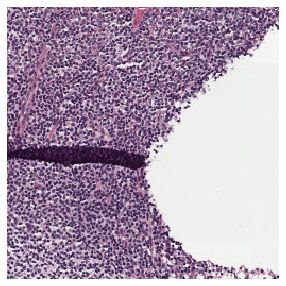
Ian Goodfellow, Yoshua Bengio, and Aaron Courville. Deep Learning. MIT Press, 2016. http:
  //www.deeplearningbook.org.

Bo Han, Quanming Yao, Xingrui Yu, Gang Niu, Miao Xu, Weihua Hu, Ivor Tsang, and Masashi
  Sugiyama. Co-teaching: Robust training of deep neural networks with extremely noisy labels. In
  Advances in Neural Information Processing Systems, pp. 8527–8537, 2018.

Martin Handford. Where’s Wally? Walker, 1987.

Kaiming He, Xiangyu Zhang, Shaoqing Ren, and Jian Sun. Deep residual learning for image
  recognition. CoRR, abs/1512.03385, 2015. URL http://arxiv.org/abs/1512.03385.

Kaiming He, Xiangyu Zhang, Shaoqing Ren, and Jian Sun. Identity mappings in deep residual
  networks. In European conference on computer vision, pp. 630–645. Springer, 2016.

Gao Huang, Zhuang Liu, Laurens Van Der Maaten, and Kilian Q Weinberger. Densely connected
  convolutional networks. In Proceedings of the IEEE conference on computer vision and pattern
  recognition, pp. 4700–4708, 2017.

Maximilian Ilse, Jakub M Tomczak, and Max Welling. Attention-based deep multiple instance
 learning. arXiv preprint arXiv:1802.04712, 2018.

Sergey Ioffe and Christian Szegedy. Batch normalization: Accelerating deep network training
  by reducing internal covariate shift. In Proceedings of the 32Nd International Conference on
  International Conference on Machine Learning - Volume 37, ICML’15, pp. 448–456. JMLR.org,
  2015. URL http://dl.acm.org/citation.cfm?id=3045118.3045167.

Stanisław Jastrz˛ebski, Zachary Kenton, Devansh Arpit, Nicolas Ballas, Asja Fischer, Yoshua Bengio,
  and Amos Storkey. Three factors influencing minima in sgd. arXiv preprint arXiv:1711.04623,
  2017.

Lu Jiang, Zhengyuan Zhou, Thomas Leung, Li-Jia Li, and Li Fei-Fei. Mentornet: Learning
  data-driven curriculum for very deep neural networks on corrupted labels. arXiv preprint
  arXiv:1712.05055, 2017.

Angelos Katharopoulos and François Fleuret. Processing megapixel images with deep attention-
  sampling models. arXiv preprint arXiv:1905.03711, 2019.

Alex Krizhevsky. Learning multiple layers of features from tiny images. Technical report, 2009.

Alex Krizhevsky, Ilya Sutskever, and Geoffrey E Hinton.    Imagenet classification with
  deep convolutional neural networks. In F. Pereira, C. J. C. Burges, L. Bottou, and
  K. Q. Weinberger (eds.), Advances in Neural Information Processing Systems 25, pp.
  1097–1105. Curran Associates, Inc., 2012. URL http://papers.nips.cc/paper/
  4824-imagenet-classification-with-deep-convolutional-neural-networks.
  pdf.

Yann LeCun and Yoshua Bengio. The handbook of brain theory and neural networks. chapter
  Convolutional Networks for Images, Speech, and Time Series, pp. 255–258. MIT Press, Cambridge,
  MA, USA, 1998. ISBN 0-262-51102-9. URL http://dl.acm.org/citation.cfm?id=
  303568.303704.

Yann Lecun, Léon Bottou, Yoshua Bengio, and Patrick Haffner. Gradient-based learning applied to
  document recognition. In Proceedings of the IEEE, pp. 2278–2324, 1998.

Byungjae Lee and Kyunghyun Paeng. A robust and effective approach towards accurate metastasis
  detection and pn-stage classification in breast cancer. CoRR, abs/1805.12067, 2018. URL http:
  //arxiv.org/abs/1805.12067.

Tsung-Yi Lin, Michael Maire, Serge Belongie, James Hays, Pietro Perona, Deva Ramanan, Piotr
  Dollár, and C Lawrence Zitnick. Microsoft COCO: Common objects in context. In European
  conference on computer vision, pp. 740–755. Springer, 2014.

                                                10
Dhruv Mahajan, Ross Girshick, Vignesh Ramanathan, Kaiming He, Manohar Paluri, Yixuan Li,
Ashwin Bharambe, and Laurens van der Maaten. Exploring the limits of weakly supervised
pretraining. In Proceedings of the European Conference on Computer Vision (ECCV), pp. 181–196,
2018.
Volodymyr Mnih, Nicolas Heess, Alex Graves, et al. Recurrent models of visual attention. In
Advances in neural information processing systems, pp. 2204–2212, 2014.
Roman Novak, Yasaman Bahri, Daniel A. Abolafia, Jeffrey Pennington, and Jascha Sohl-Dickstein.
Sensitivity and generalization in neural networks: an empirical study. In International Confer-
ence on Learning Representations, 2018. URL https://openreview.net/forum?id=
HJC2SzZCW.
Maxime Oquab, Léon Bottou, Ivan Laptev, and Josef Sivic. Is object localization for free?-weakly-
supervised learning with convolutional neural networks. In Proceedings of the IEEE Conference
on Computer Vision and Pattern Recognition, pp. 685–694, 2015.
Jiangmiao Pang, Cong Li, Jianping Shi, Zhihai Xu, and Huajun Feng. R2 -cnn: Fast tiny object
detection in large-scale remote sensing images. arXiv preprint arXiv:1902.06042, 2019.
S. Resta, N. Acito, M. Diani, G. Corsini, T. Opsahl, and T. V. Haavardsholm. Detection of small
changes in airborne hyperspectral imagery: Experimental results over urban areas. In 2011 6th
International Workshop on the Analysis of Multi-temporal Remote Sensing Images (Multi-Temp),
pp. 5–8, July 2011. doi: 10.1109/Multi-Temp.2011.6005033.
Arnaud Arindra Adiyoso Setio, Alberto Traverso, Thomas de Bel, Moira S.N. Berens, Cas van den
Bogaard, Piergiorgio Cerello, Hao Chen, Qi Dou, Maria Evelina Fantacci, Bram Geurts, Rob-
bert van der Gugten, Pheng Ann Heng, Bart Jansen, Michael M.J. de Kaste, Valentin Kotov,
Jack Yu-Hung Lin, Jeroen T.M.C. Manders, Alexander Satora-Mengana, Juan Carlos Garca-
Naranjo, Evgenia Papavasileiou, Mathias Prokop, Marco Saletta, Cornelia M Schaefer-Prokop,
Ernst T. Scholten, Luuk Scholten, Miranda M. Snoeren, Ernesto Lopez Torres, Jef Vandemeule-
broucke, Nicole Walasek, Guido C.A. Zuidhof, Bram van Ginneken, and Colin Jacobs. Vali-
dation, comparison, and combination of algorithms for automatic detection of pulmonary nod-
ules in computed tomography images: The luna16 challenge. Medical Image Analysis, 42:1
– 13, 2017. ISSN 1361-8415. doi: https://doi.org/10.1016/j.media.2017.06.015. URL http:
//www.sciencedirect.com/science/article/pii/S1361841517301020.
K. Simonyan and A. Zisserman. Very deep convolutional networks for large-scale image recognition.
CoRR, abs/1409.1556, 2014.
John Suckling. The mammographic image analysis society digital mammogram database”exerpta
medica. Exerpta Medica International Congress Series, 1069, 01 1994.
Carole H Sudre, Beatriz Gomez Anson, Silvia Ingala, Chris D Lane, Daniel Jimenez, Lukas Haider,
Thomas Varsavsky, Lorna Smith, H Rolf Jäger, and M Jorge Cardoso. 3d multirater rcnn for
multimodal multiclass detection and characterisation of extremely small objects. arXiv preprint
arXiv:1812.09046, 2018.
Chen Sun, Abhinav Shrivastava, Saurabh Singh, and Abhinav Gupta. Revisiting unreasonable
effectiveness of data in deep learning era. In Proceedings of the IEEE international conference on
computer vision, pp. 843–852, 2017.
T. Tieleman and G. Hinton. Lecture 6.5—RmsProp: Divide the gradient by a running average of its
recent magnitude. COURSERA: Neural Networks for Machine Learning, 2012.
Naofumi Tomita, Behnaz Abdollahi, Jason Wei, Bing Ren, Arief Suriawinata, and Saeed Hassanpour.
Finding a needle in the haystack: Attention-based classification of high resolution microscopy
images. arXiv preprint arXiv:1811.08513, 2018.
Dmitry Ulyanov, Andrea Vedaldi, and Victor S. Lempitsky. Instance normalization: The missing
ingredient for fast stylization. CoRR, abs/1607.08022, 2016.
11Jason W. Wei, Laura J. Tafe, Yevgeniy A. Linnik, Louis J. Vaickus, Naofumi Tomita, and Saeed
Hassanpour. Pathologist-level classification of histologic patterns on resected lung adenocarcinoma
slides with deep neural networks. CoRR, abs/1901.11489, 2019. URL http://arxiv.org/
abs/1901.11489.
Gui-Song Xia, Xiang Bai, Jian Ding, Zhen Zhu, Serge Belongie, Jiebo Luo, Mihai Datcu, Marcello
Pelillo, and Liangpei Zhang. Dota: A large-scale dataset for object detection in aerial images. In
The IEEE Conference on Computer Vision and Pattern Recognition (CVPR), June 2018.
Chiyuan Zhang, Samy Bengio, Moritz Hardt, Benjamin Recht, and Oriol Vinyals. Understanding
deep learning requires rethinking generalization. 2017. URL https://arxiv.org/abs/
1611.03530.
12Supplementary Material for
Needles in Haystacks: On Classifying Tiny Objects in Large Images
A DATASETS
In this section, we provide additional details about the datasets used in our experiments.
A.1 N EEDLE MNIST
The needle MNIST (nMNIST) dataset is designed as a binary classification problem: Is there a 3 in
this image?’. To generate nMINST, we use the original training, validation and testing splits of the
MNIST dataset and generate different nMINST subsets by varying the object-to-image (O2I) ratio,
resulting in O2I ratios of 19.1%, 4.8%, 1.2%, 0.3%, and 0.075%. We define positive images as the
ones containing exactly one digit 3 and negative images as images without any instance of it. We keep
the original MNIST digit size and place digits randomly onto a clear canvas to generate a sample of
the nMNIST dataset. More precisely, we adapt the O2I ratio by changing the the canvas size, resulting
in nMNIST image resolution being in 64 × 64, 128 × 128, 256 × 256, 512 × 512, and 1024 × 1024
pixels. To assign MNIST digits to canvas, we split the MNIST digits into two subsets: digit-3
versus clutter (any digit from a set of {0, 1, 2, 4, 5, 6, 7, 8, 9}). For the positive nMNIST images, we
sample one digit 3 (without replacement) and n digits (with replacement) from the digit-3 and clutter
subsets, respectively. For the negative nMNIST images, we sample n + 1 instances from the clutter
subset. We adapt n to keep approximately constant object density for all canvas and choose n to be
2, 5, 25, 100, and 400 for canvas resolutions 64 × 64, 128 × 128, 256 × 256, 512 × 512, and 1024 ×
1024, respectively. As result, for each value of O2I ratio, we obtain 11276, 1972, 4040 of training,
validation and testing images, out of which 50% are negative and 50% are positive images. We
present both positive and negative samples for different O2I ratios in Figure 10.
(a) O2I ratio = 19.1% (b) O2I ratio = 4.7% (c) O2I ratio = 1.2% (d) O2I ratio = 0.3% (e) O2I ratio = 0.075%
(f) O2I ratio = 19.1% (g) O2I ratio = 4.7% (h) O2I ratio = 1.2% (i) O2I ratio = 0.3% (j) O2I ratio = 0.075%
Figure 10: Example images from our MNIST dataset with different O2I ratios. Top row images
represent positive examples — digit 3 is present (marked with red rectangle), while bottom row
depicts negative images. Note that for visualization purposes all images have been rescaled to the
same resolution.
A.2 N EEDLE CAMELYON
The needle CAMELYON (nCAMELYON) is designed as a binary classification task: Are there breast
cancer metastases in the image or not?. We rely on the pixel-level annotations within CAMELYON
to extract samples for nCAMELYON. We use downsampling level 3 from the original whole slide
image using the MultiResolution Image interface released with the original CAMELYON dataset.
For positive examples, we identify contiguous regions within the annotations, and take 50 random
crops around each contiguous region ensuring that the full contiguous region is inside the crop, and
13(a) O2IR ∈ [50 − 100]% (b) O2IR ∈ [10 − 50]% (c) O2IR ∈ [1 − 10]% (d) O2IR ∈ [0.1 − 1]% (e) Negative Example
(f) O2IR ∈ [50 − 100]% (g) O2IR ∈ [10 − 50]% (h) O2IR ∈ [1 − 10]% (i) O2IR ∈ [0.1 − 1]% (j) Negative Example
(k) O2IR ∈ [50 − 100]% (l) O2IR ∈ [10 − 50]% (m) O2IR ∈ [1 − 10]% (n) O2IR ∈ [0.1 − 1]% (o) Negative Example
Figure 11: Example images from our CAMELYON dataset for different crop sizes and O2I ratios.
We show crops with size 128 × 128, 256 × 256, and 512 × 512 in the top, middle, and bottom row,
respectively. The green outlines show the cancerous regions. Note that for visualization purposes all
images have been rescaled to same resolution.
total number of lesion pixels inside the crop are in the desired O2I ratio. The negative crops are
taken from healthy images randomly filtering for images that are mostly background using a heuristic
that the average green pixel value in the crop is below 200. Since the CAMELYON dataset contains
images acquired by 5 different centers, we split training, validation and test sets center-wise to avoid
any contamination of data across the three sets. All crops coming from center 3 are part of the
validation set, and all crops coming from center 4 are part of the test set. All images are generated
for resolutions 128 × 128, 256 × 256, 512 × 512, and 1024 × 1024 and are split into 4 different O2I
ratios: (100 − 50)%, (50 − 10)%, (10 − 1)%, and (1 − 0.1)%. Figure 11 shows examples of images
from nCAMELYON dataset, Table 1 presents number of unique lesions in each dataset, and Table 2
depicts number of dataset images stratified for image resolution and O2I ratios. Because center 3 does
not contain lesions of suitable size for crops of with resolution 128 × 128 and O2I ratio (50 − 100)%,
we do not include those training runs in our analysis.
Table 1: Number of unique lesions extracted for each set of the nCAMELYON data for differen O2I
ratios and crop sizes.
Crop Size 128 256 512
O2I ratio Train Val Test Train Val Test Train Val Test
(50 - 100)% 20 0 8 27 2 13 23 5 13
(10 - 50)% 84 12 16 101 16 15 68 15 17
(1 - 10)% 176 17 18 227 17 18 235 21 15
(0.1 - 1)% 33 5 5 93 16 9 173 20 11
14Table 2: Number of crops extracted for each set of the nCAMELYON data for differen O2I ratios and
crop sizes. Note that the dataset is balanced (e. g. 50% are positive images and 50% are negative).
Moreover, for positive images we have relatively small number of unique cancer regions as noted in
Table 1.
Crop Size 128 256 512
O2I ratio Train Val Test Train Val Test Train Val Test
(50 - 100)% 1000 0 400 1350 100 650 1150 250 650
(10 - 50)% 4200 600 800 5050 800 750 3400 750 850
(1 - 10)% 8686 850 900 11270 850 900 11750 1050 750
(0.1 - 1)% 1488 247 207 4255 800 450 8312 965 550
negative 19608 6000 6100 19595 6000 6100 19574 6000 6100
B E XPERIMENTAL S ETUP
In this section, we provide additional details about the pipeline used in the experiments. More
precisely, we formally define global pooling operations and provide detailed description of the
different architectures.
B.1 G LOBAL POOLING OPERATIONS
In our experiments, we are testing four different global pooling functions: max-pooling, mean-
pooling, logsumexp and soft attention. The max pooling operation simply returns the maximum
value per each channel in the topological embedding. This operation can be formally defined
as: EI = maxw maxh Et[w,h] . Note, that we use subscript notation to denote dimensions of the
embedding. The max pooling operation has a spacing effect on gradient backpropagation, during the
backward pass through the model all information will be propagated through the embedding position
that corresponds to the maximal value. In order to improve gradient backpropagation, one could
apply logsumexp pooling, a soft approximation to max pooling. This pooling operation is defined as:
w
Xenc h
Xenc
EI = log exp Et[w,h] . (1)
w=1 h=1
Alternatively, one could use an average pooling operation that computes mean value for each channel
in the topological embedding. This pooling operation can be formally defined as follows:
wenc henc
1 1 X X
EI = Et[w,h] . (2)
wenc henc w=1 h=1
Finally, attention based pooling include additional weighting tensor a of dimension (wenc × henc ×
cenc ) that rescales each topological embedding before averaging them. This operation can be formally
defined as:
w
Xenc h
Xenc
EI = a[w,h] · Et[w,h] (3)
w=1 h=1
w
Xenc h
Xenc
s.t. a[w,h] = 1 (4)
w=1 h=1
In our experiments, following Ilse et al. (2018), we parametrize the soft-attention mechanisms
as a[w,h] = sof tmax(f (Espat ))[w,h] , where f (·) is modelled by two fully connected layers with
tanh-activation and 128 hidden units.
B.2 M ODEL ARCHITECTURE DETAILS
We adapt the BagNet architecture proposed in (Brendel & Bethge, 2019). An overview of the
architectures for the tested three receptive field sizes is shown in Table 3. We depict the layers of
15Figure 12: Impact of the training set balance on model accuracy for different pooling operations and
receptive field sizes.
residual blocks in brackets and perform downsampling using convolutions with stride 2 within the
first residual block. Note that the architectures for different receptive fields differ in the number of
3 × 3 convolutions. The rightmost column shows a regular ResNet-50 model. The receptive field
is decreased by replacing 3 × 3 convolutions with 1 × 1 convolutions. We increase the number of
convolution filters by a factor of 2.5 if the receptive field is reduced to account for the loss of the
trainable parameters. Moreover, when testing different network capacities we evenly scale the number
of convolutional filters by multiplying with a constant factor of s ∈ {1/4, 1/2, 1, 2}.
C A DDITIONAL RESULTS
In this section, we provide additional experimental results as well as additional visualizations of the
experiments presented in the main body of the paper.
C.1 C LASS - IMBALANCED CLASSIFICATION
In many medical imaging datasets, it is common to be faced with class-imbalanced datasets. Therefore,
in this experiment, we use our nMNIST dataset and test CNNs generalization under moderate and
severe class imbalanced scenario. We alter the training set class balance by altering the proportion
of positive images in the training dataset and use the following balance values 0.01, 0.1, 0.25, 0.5,
0.75, 0.9 and 0.99, where a value of 0.01 means almost no positive examples and 0.99 indicates very
low number of negative images available at training time. Moreover, we ensure that the dataset size
is constant (≈ 11k) and only the class-balance is modified. We run the experiments using the O2I
ratio of 1.2%, three receptive field sizes (9 × 9, 33 × 33 and 177 × 177 pixels) and four pooling
operations (mean, max, logsumexp and soft attention). For each balance value, we train 6 models
using 6 random seeds and we oversample the underrepresented class. The results are depicted in
Figure 12. We observe that the model performance drops as the the training data becomes more
unbalanced and that max pooling and logsumexp seem to be the most robust to the class imbalance.
C.2 I NCREASE OF MODEL CAPACITY FOR SMALL DATASET SIZES .
We also tested the effect of model capacity increase while having access only to a small dataset (3k
class-balanced images) and contrast it with a larger dataset of ≈ 11k training images. We run this
experiment on the nMNIST dataset using a network with 2.3 · 107 parameters using global max
pooling operation and there different receptive field sizes: 9 × 9, 33 × 33 and 177 × 177 pixels. The
results are depicted in Figure 13. It can be seen that the model’s capacity increase does not lead to
better generalization, for small size datasets of ≈ 3k.
C.3 O2I LIMIT VS . DATASET SIZE
In this section, we report additional results for all tested global pooling operations on O2I limit vs.
dataset size. We plot a heatmaps representing the validation set results for all considered 02I and
training set sizes (Figure 14) as well as the minimum number of training examples required to achieve
a validation accuracy of 70% and 85% (Figure 15)
16Figure 13: Impact of the network capacity on the generalization performance dependent on the
training set size for nMNIST at O2I ratio = 1.2%. The improvement based on the increased network
capacity shrinks with smaller training set.
Figure 14: Testing the O2I limit. Validation set accuracy heatmap for max, logsumexp, mean and
soft attention poolings. We test training set sizes ∈ {1400, 2819, 5638, 7500, 11276, 22552} and
report the average validation accuracy.
C.4 W EAKLY SUPERVISED OBJECT DETECTION : N MNIST
We test the object localization capabilities of the trained classification models by examining their
saliency maps. Figure 16 shows examples of the nMNIST dataset with the object bounding box in
Figure 15: Testing the O2I limit. Minimum required training set size to achieve the noted valida-
tion accuracy. We test training set sizes ∈ {1400, 2819, 5638, 7500, 11276, 22552} and report the
minimum amount of training examples that achieve a specific validation performance pooling over
different network capacities.
17(a) y = 1, ŷ = 1 (b) y = 0, ŷ = 1 (c) y = 1, ŷ = 0 (d) y = 0, ŷ = 0
(e) y = 1, ŷ = 1 (f) y = 0, ŷ = 1 (g) y = 1, ŷ = 0 (h) y = 0, ŷ = 0
(i) y = 1, ŷ = 1 (j) y = 0, ŷ = 1 (k) y = 1, ŷ = 0 (l) y = 0, ŷ = 0
(m) y = 1, ŷ = 1 (n) y = 0, ŷ = 1 (o) y = 1, ŷ = 0 (p) y = 0, ŷ = 0
Figure 16: Example images from the nMNIST validation set and their corresponding saliency maps
in red. We generate the saliency maps by calculating the absolute of the gradients with respect to the
input image using max-pooling, a receptive field of 33, and ResNet-50 capacity. From top to bottom,
we show random examples for O2I ratios of {19.14, 4.79, 1.20, 0.30}%. We annotate the object of
interest with a blue outline. The captions show the true label y and the prediction ŷ.
18(a) (b)
Figure 17: Average precision for detecting the object of interest using the saliency maps for nMNIST.
We adapt (Oquab et al., 2015) and use the localize an object by the maximum magnitude of the
saliency. We use the magnitude of the saliency as the confidence of the detection. We count wrongly
localised objects both as false positive and false negative. For images without object of interest, the
we increase the false positive count only. We plot results for max-pooling, a receptive field of 33,
a training set with 11276 examples and ResNet-50 capacity. (a) shows the dependence of the AP
on the pooling method using RF = 33 × 33, (b) shows the dependence on the receptive field using
max-pooling.
blue and the magnitude of the saliency in red. We rescale the saliency to [0, 1] for better contrast.
However, this prevents the comparison of absolute saliency values across different images. In samples
containing an object of interest, the models correctly assign high saliency to the regions surrounding
the relevant object. On negative examples, the network assigns homogenous importance to all objects.
We localise an object of interest as the location with maximum saliency. We follow (Oquab et al.,
2015) to quantitatively examine the object detection performance using the saliency maps of the
models. We plot the corresponding average precision in Figure 17. We find that the detection
performance deteriorates for smaller O2I ratios regardless of the method. This is aligned with the
classification accuracy. For small O2I ratios, max-pooling achieves the best detection scores. On
larger O2I ratios, logsumexp achieves the best scores.
C.5 W EAKLY SUPERVISED OBJECT DETECTION : N CAMELYON
We qualitatively show object detection on nCAMELYON in Figures 18 19 20 21, for True Positives,
True Negatives, False Positives and False Negatives. We observe weak correlation between segmenta-
tion maps and saliency maps, signifying that the classifier was able to focus on the object of interest
instead of looking at superficial signals in the data.
19(a) (b)
(c) (d)
(e) (f)
Figure 18: Example True Positive Images of nCAMELYON validation sets and their corresponding
segmentation maps with saliencies overlaid.
20(a) (b)
Figure 19: Example True Negative Image of nCAMELYON validation sets and corresponding
saliency map.
(a) (b)
Figure 20: Example False Negative Image of nCAMELYON validation sets and corresponding
segmentation map with saliency overlaid.
(a) (b)
Figure 21: Example False Positive Image of nCAMELYON validation sets and corresponding saliency
map.
21You can also read