Vehicle Detection of Multi-source Remote Sensing Data Using Active Fine-tuning Network
←
→
Page content transcription
If your browser does not render page correctly, please read the page content below
Vehicle Detection of Multi-source Remote Sensing Data Using
                                                          Active Fine-tuning Network
                                              Xin Wua , Wei Lia *, Danfeng Hongb , Jiaojiao Tianb , Ran Taoa , Qian Duc
                                          a
                                            School of Information and Electronics, Beijing Institute of Technology, 100081 Beijing, China,
                                                and Beijing Key Laboratory of Fractional Signals and Systems, 100081 Beijing, China
                                                                 (*corresponding author, e-mail: liwei089@ieee.org)
                                         b
                                           Remote Sensing Technology Institute (IMF), German Aerospace Center (DLR), 82234 Wessling,
arXiv:2007.08494v1 [cs.CV] 16 Jul 2020

                                                                                     Germany
                                           c
                                             Department of Electrical and Computer Engineering, Mississippi State University, Mississippi
                                                                              State, 39762 MS, USA

                                         Abstract
                                         This is a pre-print of a paper accepted by ISPRS Journal Photogrammetry and Re-
                                         mote Sensing. Please note that compared to the published version, we corrected sev-
                                         eral F1-Scores in Tables (marked in red) due to miscalculation.
                                             Vehicle detection in remote sensing images has attracted increasing interest in
                                         recent years. However, its detection ability is limited due to lack of well-annotated
                                         samples, especially in densely crowded scenes. Furthermore, since a list of remotely
                                         sensed data sources is available, efficient exploitation of useful information from
                                         multi-source data for better vehicle detection is challenging. To solve the above
                                         issues, a multi-source active fine-tuning vehicle detection (Ms-AFt) framework is
                                         proposed, which integrates transfer learning, segmentation, and active classification
                                         into a unified framework for auto-labeling and detection. The proposed Ms-AFt
                                         employs a fine-tuning network to firstly generate a vehicle training set from an unla-
                                         beled dataset. To cope with the diversity of vehicle categories, a multi-source based
                                         segmentation branch is then designed to construct additional candidate object sets.
                                         The separation of high quality vehicles is realized by a designed attentive classifica-
                                         tions network. Finally, all three branches are combined to achieve vehicle detection.
                                         Extensive experimental results conducted on two open ISPRS benchmark datasets,
                                         namely the Vaihingen village and Potsdam city datasets, demonstrate the superior-
                                         ity and effectiveness of the proposed Ms-AFt for vehicle detection. In addition, the
                                         generalization ability of Ms-AFt in dense remote sensing scenes is further verified on
                                         stereo aerial imagery of a large camping site.
                                         Keywords: Multi-source, vehicle detection, optical remote sensing imagery,

                                         Preprint submitted to ISPRS Journal of Photogrammetry and Remote Sensing           July 17, 2020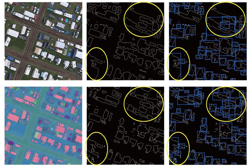
fine-tuning, segmentation, active classification network

1. Introduction
    Recently, vehicle detection in remote sensing has been garnering growing atten-
tion and has been successfully applied in many applications, such as traffic man-
agement (Arivalagan and Venkatachalapathy, 2015; Karim et al., 2014), and urban
planning (Wen et al., 2019; Weng et al., 2018). Visible (VIS) remote sensing im-
agery uses electromagnetic wave imaging at a wavelength of 400 ∼ 760 nm, which
visually reflects the true color and texture of vehicle objects. Inspired by the recent
advancement of deep learning and availability of multi-source remote sensing, such
as RGB, hyperspectral (Hong et al., 2019a), multispectral (Weng et al., 2014), and
synthetic aperture radar (SAR) (Kang et al., 2020), many state-of-the-art vehicle
detection algorithms in remote sensing (Cheng et al., 2018; Yang et al., 2018; Wu
et al., 2019; Kang and Gellert, 2015; Audebert et al., 2017; Gintautas et al., 2009;
Wei et al., 2013; Cheng et al., 2020; Wu et al., 2020) have been developed.
    The success of using VIS images depends on the strong support of large-scale and
accurate annotated datasets, e.g., NWPU VHR-10 dataset (Cheng et al., 2014, 2016;
Cheng and Han, 2016) 1 , DOTA dataset (Xia et al., 2018) 2 , and DIOR dataset (Li
et al., 2020) 3 . However, vehicles in VIS imagery are prone to have more complex
deformation (see Fig. 1), due to its “bird” perspective. This inevitably increases the
cost of manual annotation, thereby yielding a bottleneck. In order to solve this prob-
lem, a series of transfer learning (Chen et al., 2018b), semi-supervised (Chen et al.,
2018a), weakly-supervised (Han et al., 2015) and even unsupervised methods were
successively developed to reduce the cost of annotation. A novel weakly-supervised
framework was proposed based on Bayesian principles for vehicle detection from VIS
images (Han et al., 2015). In (Chen et al., 2018a; Lin et al., 2016), the generative
adversarial network (GAN) has shown its superiority in data augmentation. GAN
was developed to extract data distribution from unlabeled images in order to realize
semi-supervised airplane detection (Chen et al., 2018a). Furthermore, multiple-layer
feature-matching generative adversarial networks (MARTA GANs) were designed to
learn a representation using only unlabeled data to realize object classification (Lin
et al., 2016). Subsequently, with a growing attention in limited or without labels,
considerable work for object detection in remote sensing imagery has been reported

  1
    http://www.escience.cn/people/gongcheng/NWPU-VHR-10.html.
  2
    https://captain-whu.github.io/DOTA/dataset.html.
  3
    http://www.escience.cn/people/gongcheng/DIOR.html.

                                          2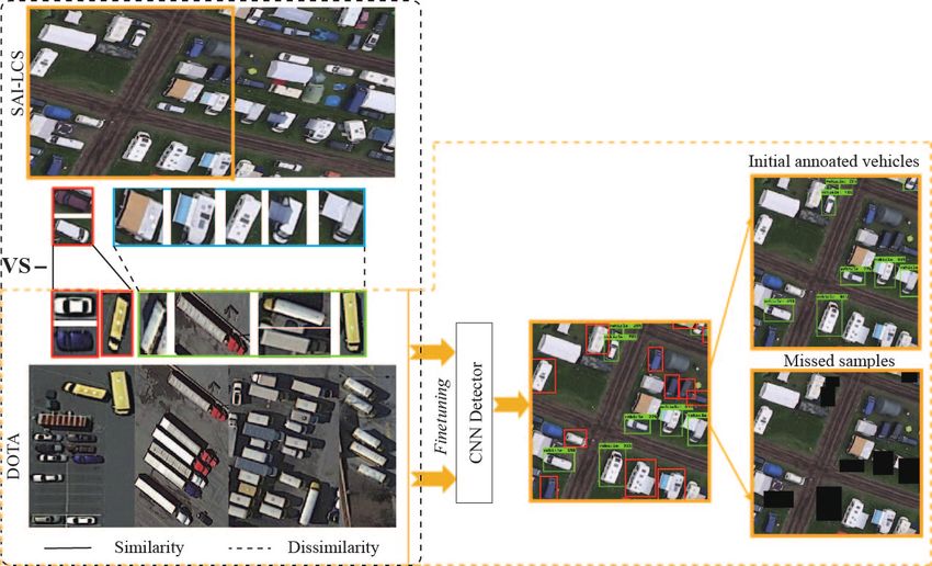
I. Fine-tuning Deep Detection
RGB Image Refine-tuning with Scene-specific detection network
Preliminary Detection Final Detection Result
Non-Maximum Suppression
Detections
Vehicle
Vehicle
II. Segmentation in Merged Image III. Active Classification Network
DSM Image Merge Candidate Objects
High-quality Vehicles
1 2
1.Tent
2.Vehicle
Full Connect
Training
Softmax
Relu
Testing
Segmentation Region Selection Location Binary Clssification
Figure 1: The overall flowchart of the proposed Ms-AFt, including automatic labeling and vehicle
detection in complex remote sensing scene. More specifically, we first use a pre-trained detection
network trained on other data sources (e.g., ImageNet), and the preliminary detection results of
our unlabeled datasets can then be obtained by directly using the network. Next, an unsupervised
object-based segmentation is performed using fused RGB and DSM images and potential objects
can be screened out by the means of height information. Subsequently, these selected objects can be
further classified into vehicles or non-vehicles using the branch III, i.e., active classification network.
Finally, those high-quality vehicles with their location information are re-fed into the deep detection
network to finely tune the network parameters.
in the literature (Aldeborgh et al., 2017; Cao et al., 2016). Despite this, the detection
ability using only a single data source still remains limited, due to the lack of feature
diversity. For this reason, the joint use of multi-source data might be a good solution
(Hong et al., 2019b).
With the development of airborne sensors (Sumbul et al., 2019), the quantity and
quality of remote sensing images have been greatly improved, which can make up,
to some extent, for the limited performance of using a single data source. Some re-
searchers have developed some work using multi-source data to achieve more accurate
vehicle detection (Schilling et al., 2018), but there is still room for improvement. Re-
cently, digital surface models (DSM) have shown great potential in object detection.
They can collect elevation information of objects and truly represents the ground ups
and downs, yielding an effective separation of objects and background. There are
two primary ways to generate DSM, namely LiDAR and photogrammetry. Among
3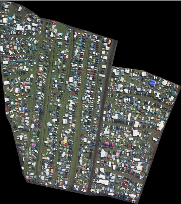
them, DSM obtained by LiDAR (Huang et al., 2020) has uniformity and high pre-
cision, but objects at the same location, especially for moving objects, rarely have
LiDAR and aerial images at the same time. In addition, LiDAR equipment is expen-
sive, so it is difficult to promote it in some practical applications. Thankfully, DSM
obtained by photogrammetry (Chai, 2016), that is reconstructing DSM directly on
multi-view images or video data acquired by manned aircraft or UAV, can greatly
reduce the cost and has been successfully applied in change detection, building ex-
traction, auxiliary vehicle testing and other fields in recent years. A classification
framework by combining morphological profiles, a spatial transformer network (STN)
and a convolutional neural network (CNN) (Rasti et al., 2020) has been proposed
for LiDAR-DSM data classification (He et al., 2019).
    Inspired by the aforementioned investigation, we expect to further improve the
detection performance of VIS images by taking the DSM as an auxiliary data source.
Therefore, we do not extensively rely on the quality of DSM, as long as the used DSM
can provide the performance improvement on the basis of that using VIS images. In
other words, even though the DSM suffers from the effects that lead to the image
degradation, e.g., slight move or missing of certain objects, tiny shift between VIS
and DSM in the process of imaging or alignment, the quality of DSM is acceptable in
our task. We have to admit, however, that the DSM with high quality can improve
the detection results more effectively but also brings greater expense. As a trade-off,
some existing datasets including DSM and VIS images, to a great extent, can meet
our requirements.
    In summary, VIS remote sensing imagery is sensitive to lighting, occlusion, and
weather changes, so its ability to extract distinguishable features is still limited.
DSM can work regardless of natural illumination. In order to effectively overcome
the lack of distinguishability of a single sensor, data fusion is employed to make full
use of the complementary information between multi-source images (Hong et al.,
2019c). Existing multi-source data-based methods (Marmanis et al., 2016; Niessner
et al., 2017; Hendrik et al., 2018) use pre-fusion or post-fusion multiple sensor data
under a supervised framework to improve the network’s ability in feature learning
rather than assisting in object detection. The main purpose of this paper is to
realize vehicles auto-labeling to improve detection performance. Generally, it is very
expensive and time-consuming to construct a large number of training samples for
object detection. Therefore, it is meaningful but challenging to detect vehicles with
an unlabeled training set.
    To overcome these difficulties, a multi-source vehicle detection framework using
an active fine-tuning network, Ms-AFt for short, is proposed. The proposed Ms-
AFt network inherits the advantages of multi-source images, yielding more accurate

                                          4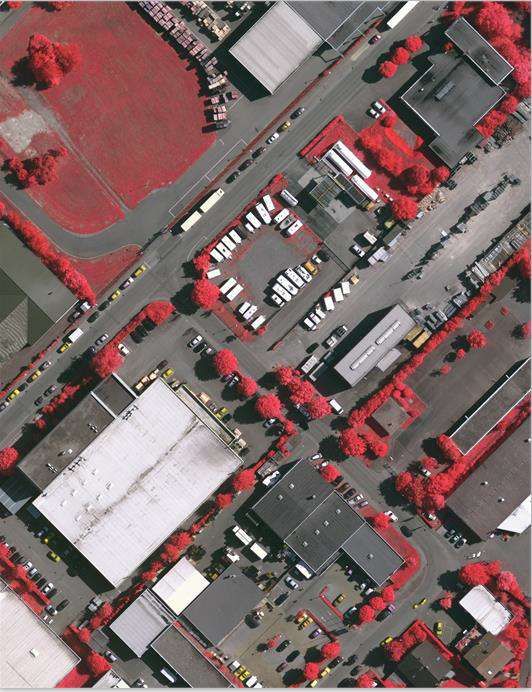
Figure 2: Illustration of the fine-tuning branch. Vehicle samples are shown within the dashed lines
of a DOTA and SAI-LCS.

labels of vehicle objects and higher detection performance. More specifically, the
main contributions of this paper can be summarized as follow:
    • To overcome the disadvantages of a single data source in vehicle detection, a
      strategy of using multi-source data is developed. Specially, DSM data with-
      out any label information are used to assist in locating ground objects in the
      segmentation branch to construct a vehicle candidate set.
    • Around multi-source data, the proposed Ms-AFt subtly integrates transfer
      learning, objects segmentation and active classification into a unified frame-
      work, ensuring vehicle auto-labeling with complementary information.
    • In the proposed Ms-AFt, an active classification network is designed, which can
      effectively screen high quality vehicles to increase the diversity and number of
      training sets with progressive improvement in vehicle detection.
   The remainder of this paper is organized as follows. Section 2 describes the three
branches of the proposed unlabeled vehicle detection framework, including transfer

                                                5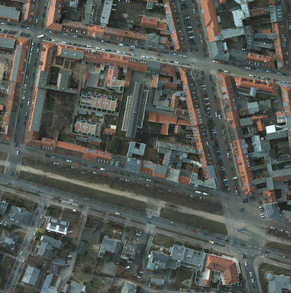
learning, object segmentation and active classification. Section 3 validates the pro-
posed framework and reports detection results, as compared with six competitive
networks. Section 4 draws the conclusions and briefly discusses future work.

2. Proposed Vehicle Detection Framework
    As illustrated in Fig. 1, the proposed Ms-AFt network consists of three branches.
They are the fine-tuning branch, segmentation branch, and active classification
branch. In the first branch, VIS images are fed into a pre-trained network to gen-
erate the first part of the vehicles training sets. To enrich the diversity of vehicle
categories, the multi-source based segmentation branch is designed to generate addi-
tional candidate object sets. Then, an active classification network with the classic
ResNet18 architecture is used to classify different objects, e.g., buildings, tents, ve-
hicles, and further screen out the high-quality vehicles from candidate object sets.
These selected candidates can be augmented to the vehicle training set and used to
finely tune the designed detection network for the final vehicle detection.

2.1. Fine-tuning Branch
    As the data used in practice are usually unlabeled, we attempt to answer the
following question: How can we implement vehicle detection similar to world-class
images? In transfer learning, a reference dataset and a target dataset are sufficiently
similar, and the reference dataset is often much larger than the target dataset. There-
fore, a pre-training network is introduced and fine-tuned - only the Dataset for Object
deTection in Aerial (DOTA) images with the annotation information containing at
least one vehicle object while keeping the other configurations of the network the
same, yielding a detection result for the unlabeled dataset. DOTA is an aerial image
dataset with 15 categories of objects collected by Wuhan University, Huazhong Uni-
versity of Science, and Technology and the German Aerospace Center. This dataset
contains 2806 aerial images from different sensors and platforms and 188,282 fully
annotated objects. Each image is of size about 4000 × 4000 pixels. So far, it is
the largest open-sourced labeling dataset in the field of remote sensing for object
detection.
    In terms of limited datasets, computing resources, and time, using a pre-trained
model is the best choice. Existing work (Lin et al., 2016) has confirmed experimen-
tally that a model trained from scratch cannot surpass the fine-tuned model based
on a pre-trained network. Some representative pre-trained networks, which are listed
in Section 3.3 and used in this paper are mainly trained by a large visual dataset
(e.g., Imagenet, COCO). For the network fine-tuning, we first separate the vehicles

                                           6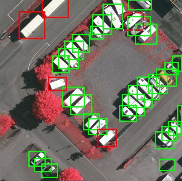
from the DOTA dataset and build a small DOTA vehicle dataset, and then the above
pre-trained networks are fine-tuned. Except that the output class number and the
learning rate are adjusted to 2 and 0.001, respectively, other network parameters
remain unchanged during network fine-tuning. For simplicity, all the layers, rather
than freezing several layers or redesigning the network, are retrained. In addition,
the final training set of the detected dataset includes all DOTA vehicle samples in
order to prevent overfitting.
    However, detection performance is closely related to the similarity between dif-
ferent datasets, which limits the generalization performance. Fig. 2 takes the Stereo
Aerial Imagery of a Large Camping Site (SAI-LCS) dataset constructed by the Ger-
man Aerospace Center as an example to show this dataset and DOTA containing
vehicle samples. As we can see, the SAI-LCS has a more complex background and a
wider variety of vehicles than DOTA. The background of the images in SAI-LCS is a
grass lawn, which greatly reduces the difference between objects and background. In
addition, there are many types of vehicles in the SAI-LCS, including recreational ve-
hicles (RVs), suspected RVs, etc, which are not in DOTA, and the objects are densely
arranged and even have adhesions. The large-scale missed alarm in the detection re-
sults as shown in Fig. 2 also confirms the above statement, so it is not sufficient for
effective vehicle detection in the SAI-LCS by simply using DOTA vehicle images for
fine-tuning.

2.2. Object Segmentation Branch
    In view of the limitations of network fine-tuning, a feasible solution to improve
vehicle detection performance for unlabeled datasets is to automatically increase the
diversity of vehicles while expanding the number of training sets. In other words,
we firstly separate objects from ground in the image, construct non-similar vehicle
candidate sets, and then use the active vehicle classification network to select high
quality vehicles. Among them, object separation is discussed in this section, and the
active classification will be discussed in Section 2.3.
    The segmentation-based method is one of the most effective methods to separate
objects from the ground. The classic pixel-based segmentation method (Zanotta
et al., 2018) is suitable for VIS images, which are disturbed by illumination, occlu-
sion, shadow, background clutter, and other factors. In addition, excessive reliance
on spectral information can also result in a large number of fractured areas, which
inevitably reduces the quality of segmentation, especially for long-range aerial im-
ages. Here, DSM is considered to compensate for the disadvantages of VIS. It covers
the terrain and other surface information except for the ground, expressing the fluc-
tuation of the ground most realistically.

                                          7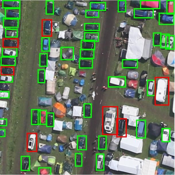
In order to make full use of multi-source image information to improve the ac-
curacy of ground object positioning, a scalar weighted fusion strategy, especially for
both sensors with high quality, is employed. For the segmentation method, object
rigid structure and adopt superpixel segmentation (Hong et al., 2020) are utilized
to achieve separation of dense ground objects. Superpixel can remove redundant
information and fit edges and its processing speed is more than ten times faster, so it
is more suitable for positioning densely arranged objects. Fig. 1 (see part II) shows
the flowchart of object segmentation. The main steps are summarized as follows.
     1) Superpixel Segmentation and Clustering: simple linear iterative clustering
(SLIC) (Achanta et al., 2012) is chosen for image superpixel segmentation. The
superpixel has good compactness and boundary fit with fast computation speed,
which well maintains the object contour (Hong et al., 2020). SLIC iterates around
distance measurement. Note that the number of superpixels in SLIC is a to-be-set
hyperparameter. In our case, the parameter is empirically and experimentally deter-
mined to be around 2000. If D between the two cluster centers is less than a certain
threshold, superpixels and corresponding adjacency matrices of each cluster can be
returned. As for the spatial aggregation, density-based spatial clustering of applica-
tions with noise (DBSCAN) (Ester et al., 1996) is considered, which does not need
to specify the number of clusters. Given the neighborhood parameters (ε, M inP ts),
the clustering result is deterministic, and it can also solve the special situation of
data distribution.
     2) Region Selection and Localization of Ground Objects: to effectively eliminate
the impact of objects with higher elevation information in the image (e.g., trees, high-
rise buildings, etc.) for the final vehicle separation, the DSM image is thresholded
to keep it within a certain height interval, and each cluster value in this image is
defined as its average height. In detail, given the to-be-selected candidates, denoted
as zi , i = 1, ...., p, from the step 1), we expect to screen out the regions (Rj (zi ), j =
1, ..., q, where p  q) with a proper size via a hard threshold (th), e.g.,
                                           (
                                            1, if area(zi ) < th,
                                Rj (zi ) =                                                (1)
                                            0, otherwise,
where the symbol area(•) is defined as the area computation of the • candidate.
Using Eq. (1), these candidates can be effectively categorized into two groups by a
given threshold, according to the order of the area size. Once the selected ground
objects are determined, the morphological filtering with dilation and erosion is used
to further smooth their edges.
    3) Vehicle Candidate Set Generation: the purpose of vehicle detection is classi-

                                             8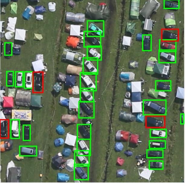
Discarded vehicles
CNN No
Vehicle (0.95)
Whether
high quality vehicles? Annotated vehicles
Vehicle (0.1)
Yes
Additional vehicle labels
Refine-tuning deep detection
Scene images
Figure 3: Illustration of the designed active classification branch. The pipeline includes CNN and
model initialization, detection training set updating, picking high-confidence samples selection and
labeling, where the arrows indicate the workflow.
3 × 3 conv, 512, /2
3 × 3 conv, 128, /2
3 × 3 conv, 256, /2
3 × 3 conv, 64
3 × 3 conv, 64
3 × 3 conv, 64
3 × 3 conv, 64
3 × 3 conv, 64
3 × 3 conv, 512
3 × 3 conv, 512
3 × 3 conv, 128
3 × 3 conv, 256
3 × 3 conv, 128
3 × 3 conv, 256
3 × 3 conv, 512
3 × 3 conv, 128
3 × 3 conv, 256
GAP
Figure 4: The detailed framework of CNN for active classification network.
fication and positioning, but the diversity of vehicle types in aerial image datasets
inevitably increases the complexity of strict vehicle positioning. Here, the smallest
circumscribed rectangle of the selected region is constructed, then a corner detector
is employed to obtain the diagonal location information of objects in each selected
region, and the horizontal bounding box location of the object is implemented.
2.3. Actively Classification Branch
As the vehicle categories are more than one, effective selection of high quality
vehicles from the vehicle candidate set are discussed in Section 2.3. An active classi-
fication network inspired by active learning is employed. Different from the classical
9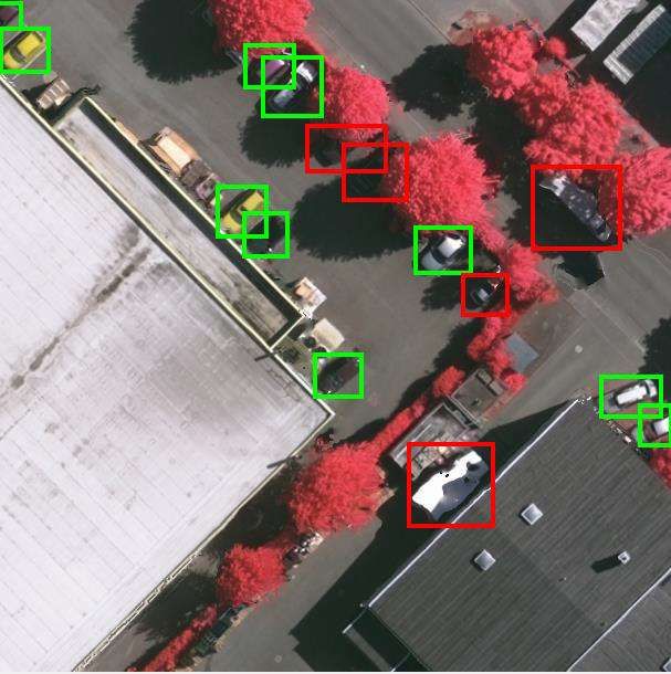
Table 1: Classification performance comparisons of four different classifiers. The best results are
highlighted in bold.
                     Dataset          Method         Precion   Recall   F1-Score
                                      VGG-19          0.93      0.67      0.78
                                     GoogleNet        0.95      0.76      0.84
                 ISPRS Vaihigen
                                    Cascadenet18      0.95      0.74      0.83
                                     ResNet18         0.96     0.86      0.91
                                      VGG-19          0.95      0.78      0.86
                                     GoogleNet        0.97      0.85      0.91
                 ISPRS Potsdam
                                    Cascadenet18      0.96      0.82      0.88
                                     ResNet18         0.99     0.90      0.94
                                      VGG-19          0.92      0.52      0.66
                                     GoogleNet        0.96      0.70      0.81
                  DLR SAI-LCS
                                    Cascadenet18      0.96      0.58      0.72
                                     ResNet18         0.97     0.76      0.86

active learning method with manual labeling by related experts, the active classi-
fication branch appoints the ResNet18 network as the active selection strategy to
automatically learn the high quality vehicles from candidate objects. This process
is called “active classification”. Fig. 3 shows the flowchart for this branch, and its
detailed steps are as follow.
    Step1: Classification Training Set Construction
    There are three parts of vehicle samples in the classification network, namely
the vehicles in DOTA, the detected vehicles in target dataset by Section 2.1, and
the manually labeled vehicles in this section. In comparison, the third part of the
classification training set plays a decisive role in the whole classification branch. It
mainly focuses on the characteristics of vehicles, including various scales, directions,
shapes, and so on, which can greatly improve the vehicle classification performance.
In the experiments, it is necessary to know the average size of vehicles (objects) for
better training the classification network.
    Step2: High Quality Vehicles Selection
    Four pre-trained classification networks are compared, namely, VGG-19 (Simonyan
and Zisserman, 2014), GoogleNet (Szegedy et al., 2017), Cascadenet18 (Pang et al.,
2017), and ResNet18 (He et al., 2016). Table 1 lists the performance of these four
classification networks. For a fair comparison, the parameters of each network are
optimized. Overall, the classification performance of ResNet18 is the best. The
possible reason is that each layer of the ResNet with shortcut connection has a sur-
vival probability, and would be discarded according to actual needs, which makes
the ResNet always yield the best performance, but the other three networks are not

                                                10
adjustable. In addition, ResNet can ease the speed of performance descent when
the resolution of the input image is fine enough. Specifically, the recall of the ISPRS
dataset is much higher than that of the DLR data set because the vehicle types of the
ISPRS dataset are more general and the existing public vehicle samples are sufficient
to cover.
By following the above analysis, ResNet18 is selected as the classification net-
work due to the fact that the resolution of vehicles is relatively small. The de-
tailed architecture of the classification network is shown in Fig. 4. Among them,
the GAP in the network is the global average pooling layer. Given a training set
S = {(x1 , y1 ) , · · · , (xN , yN )} with N samples and K categories, where xi and yi
denote the i-th sample and its corresponding label, respectively, we then define the
following cross-entropy loss LC for a binary classification task.
N
−1 X
LC = [yi logaSofti + (1 − yi )log(1 − aSofti )], (2)
N i=1
where aSoft denotes the feature outputs after going through the softmax layer.
2.4. Analysis on Proposed Ms-AFt
The recent success of CNN-based architecture brings the power in vehicle detec-
tion, owing to sufficient well-annotated samples (Yang et al., 2018; Ji et al., 2019;
Mandal et al., 2019; Schilling et al., 2018). However, costly manual labeling makes it
difficult to acquire a large number of labeled samples in practice, leading to the poor
detection performance of the previous network-based methods, e.g., FCN (Schilling
et al., 2018). Therefore, it is a feasible solution to build an effective auto-labeling
method to expand the number and categories of training samples. Also, the intro-
duction of multi-source data, e.g., DSM with height information can roughly locate
and label the ground objects inferred, can further improve the accuracy of object
auto-labeling and finally detection performance.
The proposed Ms-AFt framework mainly focuses on vehicle auto-labeling. Except
for the detection class and learning rate, the classic network architecture used in this
paper is not revisted or updated. Fig. 5 illustrates a visual example of the auto-
labeling process. The joint use of three branches in the proposed Ms-AFt network
can effectively improve the detection performance of vehicles by means of multi-
source data. In the first branch, VIS images are sent to a pre-trained network to
generate the first part of the vehicle training sets for an unlabeled dataset. To
cope with the diversity of vehicle categories, the multi-source based segmentation
branch is designed to generate additional candidate object sets. Then, an active
11Figure 5: Visualization of our vehicle auto-labeling workflow for the SAI-LCS dataset. First column:
VIS data (up) and DSM image (down). Second column: the auto-labeling results of fine-tuning
branch (up) and segmentation branch (down). Third column: the auto-labeling objects mask (up)
and high quality vehicles results (down).
classification network with the classic ResNet18 network as an automatic selection
strategy is constructed to confirm the valid category of unknown high quality vehicles
from candidate object sets, and to augment the vehicle training sample set for final
vehicle detection. In addition, the Ms-AFt framework is based on the constraint
that: 1) the labeled reference vehicle dataset is complex enough; in other words, it
can approximate the real world reflection; 2) the VIS and DSM are acquired at the
same time. Specifically, the multi-source data used in the segmentation branch is
mainly to improve the accuracy of ground objects positioning, rather than improving
the discriminability of the network. The DSM does not participate in the comparison
because it inevitably results in poor edge segmentation due to the impact of filling.
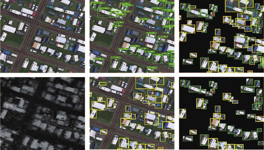
Fig. 6 illustrates an example of segmentation results. In the yellow ellipse area, it
can be visually seen that the multi-source image helps to reduce adhesion between
regions. In addition, the DSM of dark vehicles can effectively make up insufficient
contrast between vehicles and ground in the VIS image, improving the accuracy of
its positioning.
12Figure 6: An example image for auto-labeling in the segmentation branch. The first row and
second row shows the results of VIS and merged image, respectively. The yellow ellipse points to
two distinct discrimination in the visualization.
To reduce the complexity of ground object positioning, a generalized bounding
boxes positioning method, named horizontal bounding boxes (HBB), is utilized. A
common description of HBB is (xc , yc , w, h), where (xc , yc ) is the center location, w, h
are the width and height of the bounding box, respectively. In addition, regional
connectivity is examined to ensure that only one object is included in each selected
area.
3. Experimental Results and Analysis
3.1. Data Description
The performance of the proposed active fine-tuning network are quantitatively
and qualitatively evaluated on three representative multi-source datasets: two from
the ISPRS 2-D semantic segmentation baseline dataset (Vailingen village dataset4
4
http://www2.isprs.org/commissions/comm3/wg4/2d-sem-label-vaihingen.html.
13and Potsdam city dataset5 ) and the Stereo Aerial Imagery of a Large Camping Site
(SAI-LCS) dataset (Gstaiger et al., 2018). It should be noted that this paper aims at
improving the detection performance using multi-source remote sensing data, e.g.,
VIS and DSM images. Therefore, this requires a good alignment between multi-
source data. The three used datasets are generated by the photogrammetric way.
This means that the two products (VIS and DSM) are actually produced from a
single data source, e.g., aerial imagery. Such method, to a great extent, can meet the
alignment requirement. More details regarding these datasets are given as follows.
3.1.1. ISPRS 2-D Semantic Segmentation Baseline Dataset
DSM Generation Process: DSMs for ISPRS 2-D Semantic dataset is by pho-
togrammetry. This dataset consists of very high resolution orthophoto (TOP) tiles
and the corresponding DSM derived from dense image-matching techniques. Both
areas cover urban scenes. Among them, the TOP image is generated using Trim-
ble INPHO OrthoVista, and the DSM is produced by dense image matching using
Trimble INPHO 5.3 software.
Experiment Data Introduction: 1) Vaihingen Village Dataset: Vaihingen
dataset consists of 33 differently sized areas and its ground sampling distance is
9 cm. The TOP of this dataset is an 8-bit TIFF file with three bands (near in-
frared, red and green channels available). There are occlusions and shadows in the
vehicle parked area for each image. These areas constitute an opaque wall, which
greatly increases the difficulty of vehicle detection, especially for dark vehicles. In
the following experiment, the vehicle training set contains 28 aligned VIS and DSM
scene images with approximately 700 vehicles. The testing set has 5 VIS scene im-
ages with 148 manually labeled vehicle samples; 2) Potsdam City Dataset: this
dataset includes 38 differently sized areas and its ground sampling distance is 5cm.
The TOP of this dataset is an 12-bit TIFF file with four bands (near infrared, red,
green and blue channels available). Overall, there are few overlapped objects (or
occlusion) in the parking area of the image scene. Compared with the other two
data sets, vehicle detection from this image is relatively simple. In the experiment,
about 6,000 vehicles contained in 33 aligned VIS and DSM scene images are used as
the training set. The testing set has 5 VIS scene images with 1874 manually labeled
vehicle samples.
Since the main focus of this paper is to realize vehicles auto-labeling for vehicle
detection, the ground truth in this dataset is only used for testing.
5
http://www2.isprs.org/commissions/comm3/wg4/2d-sem-label-potsdam.html.
143.1.2. SAI-LCS Dataset
DSM Generation Process: DSMs for SAI-LCS dataset were collected by pho-
togrammetry. Firstly, optical imagery was collected, acquired by the optical 4K
camera system on the German Aerospace Center (Deutsches Zentrum fr Luft- und
Raumfahrt, DLR) research helicopter BO 105 (DLR (CC-BY 3.0)) at a height of
600m above the ground. The ground sampling distance (GSD) of images was around
11 cm. With three cameras on board, the 4K camera system is able to capture
the multi-view imagery with 90% overlap along-track and 60% overlap across the
track. DSMs were reconstructed by a Structure from Motion (SfM) technique, and
literature (Gstaiger et al., 2018) described these in detail.
Experiment Data Introduction: This SAI-LCS dataset is a subset from the aerial
imagery of a large camping site in northern Germany, which comprised an area of
1.0km × 1.5km. In the experiment, the vehicle training set contains 40 aligned VIS
and DSM scene images with about 900 vehicles. The testing set has 60 VIS scene
images with 2313 manually labeled vehicle samples.
3.2. Experimental Setup
In the experiment, the input image of detection is always resized to a fixed shape
of 608 × 608 pixels. For avoiding object splitting, the step size is set to 304 and
the testing result only retains IOU (Intersection over Union) >0.7. In the active
deep classification network, the resolution of the image in the vehicle candidate set
is rescaled and resampled to 60 × 60 pixels. To prevent over-fitting classification, all
the images in the training set are rotated from 0◦ to 270◦ in steps of 90◦ . In addition,
images are transformed to the HSV color space to improve the network’s robustness
to change of illumination.
Five commonly-used criteria, Precision-Recall Curve (PRC), Average Precision
(AP ), Precision (P), Recall (R), and F1-score are adopted to quantify detection
accuracy. Among them, AP is a global indicator measured by the area under the
PRC. The higher the AP value, the better the performance. The Precision (P) is
computed by T PT+FP
P
, and the Recall (R) rate is T PT+F
P
N
, TP, FP, and FN denote true
positive, false positive, and false negative, respectively. Moreover, the F1-score and
AP can be computed by using the following equations
2∗P ∗R
F1 = , (3)
(P + R)
and n
X
AP = P (k)∆R(k), (4)
k=1
15ISPRS dataset
SAI-LCS dataset
(a) Original ground truth (b) Vehicle ground truth (c) detection result
Figure 7: Qualitative evaluation of the experimental datasets. (a) is the given original ground truth
of the scene including different categories. (b) is the corresponding vehicle ground truth selected
from (a). (c) shows our vehicle detection results, where a green box denotes correct detection, a
red box denotes the leak detection.
where P (k) and ∆R(k) = R(k) − R(k − 1) denote the precision and recall difference,
respectively, when using the k-th threshold.
All the deep learning experiments are implemented with the Tensorflow frame-
work and carried out by a PC with an Intel single Core i7 CPU, NVIDIA GeForce
GTX-1080 GPU (24 GB memory), and 8 GB RAM. The PC operating system is
Ubuntu 16.04.
3.3. Experimental Results and Discussion
In the experiment, Ms-AFt has been embedded into six detection networks,
namely FRCNN ResNet101 (FRCNN-A)(Dai et al., 2016), FRCNN ResNet101 receptionV2
(FRCNN-B) (Szegedy et al., 2017), SSD (Ning et al., 2017), YOLO1 (Joseph et al.,
2016), YOLO2 (Joseph and Ali, 2017), and R-FCN ResNet101 (Dai et al., 2016), to
evaluate its detection performance. For a fair comparison, each network uses optimal
parameter settings. Fig. 7 shows the examples of vehicle reference labels selected
from the original ground truth and the corresponding detection results on two dif-
16SSD FRCNN-B FRCNN-A YOLO1 YOLO2 RFCN Thr=0.6
0.80 0.80
0.78 0.78
0.76 0.76
Precision
Precision
0.74 0.74
0.72 0.72
0.70 0.70
0.35 0.40 0.45 0.50 0.60 0.65 0.35 0.40 0.45 0.50 0.60 0.65
Recall Recall
(a) VIS Fintuning (b) Ms-AFt
Figure 8: PRCs of the proposed framework on the six example networks for the ISPRS Vaihingen
dataset.
Table 2: Performance comparisons of six networks structure for the ISPRS Vaihingen dataset. The
best results are highlighted in bold.
thr=0.6
Method Ground Truth AP Costs/s
Recall Precision F1-Score
SSD-Ft 148 0.5632 0.4005 0.6925 0.5075 0.14
YOLO1-Ft 148 0.5927 0.4126 0.7025 0.5199 0.13
YOLO2-Ft 148 0.6012 0.4258 0.7200 0.5351 0.15
VIS Images
FRCNN-A-Ft 148 0.6000 0.4089 0.7130 0.5198 5.54
FRCNN-B-Ft 148 0.5725 0.4051 0.7039 0.5142 5.98
R-FCN-Ft 148 0.6500 0.4328 0.7525 0.5495 0.32
SSD-Ms-AFt 148 0.5812 0.4221 0.7358 0.5365 0.14
YOLO1-Ms-AFt 148 0.6575 0.4225 0.7528 0.5413 0.13
YOLO2-Ms-AFt 148 0.6600 0.4521 0.7712 0.5700 0.15
Multi-source Images (VIS+DSM)
FRCNN-A-Ms-AFt 148 0.6823 0.4448 0.7821 0.5671 5.54
FRCNN-B-Ms-AFt 148 0.6455 0.4341 0.7525 0.5506 5.98
R-FCN-Ms-AFt 148 0.7277 0.4759 0.8012 0.5971 0.32
ferent datasets. The final quantified result is calculated by the overlap rate of the
reference labels and detection results.
Tables 2 - 4 provide the quantitative results for three experimental datasets,
namely AP and running cost. The objective of this paper is to achieve vehicle auto-
labeling by multi-source data while improving its detection performance. So the
threshold in PR curves should be chosen to weigh the accuracy and quantity of auto-
labeling vehicles, Tables 2 - 4 also provide the Recall, Precision, and F1-score of all
17Figure 9: Visual detection results of part areas of the ISPRS Vaihingen dataset. A green box
denotes correct detection, a red box denotes leak detection.
networks when the threshold is 0.6. Overall, the results of the three datasets are
similar. One-stage based SSD yields the worst performance. The possible reason is
that there is a serious positive and negative sample imbalance problem in the one-
stage network. Most of the anchors that the network finally learns are not conducive
to the final network learning. While in the two-stage network architecture, e.g.,
FRCNN, the number of final training anchors is only hundreds or thousands and is
useful, which can ensure the network learning optimal to the maximum. YOLO1 is a
real-time object detection framework and its detection time is about 0.14s on images
with 608 × 608 resolution; however, it is sensitive to the object with a large range of
scales and directions. Although YOLO2 improves the scale robustness of the network
by introducing the multi-scale feature map, its generalization ability still needs to be
improved for small objects. The detection performance of FRCNN with Resnet101
is better than inception resnet v2 atrous, our interpretation for this is the atrous
18SSD FRCNN-B FRCNN-A YOLO1 YOLO2 RFCN Thr=0.6
0.90 0.90
0.88 0.88
0.86 0.86
Precision
Precision
0.84 0.84
0.82 0.82
0.80 0.80
0.35 0.40 0.45 0.50 0.60 0.65 0.35 0.40 0.45 0.50 0.60 0.65
Recall Recall
(a) VIS Fintuning (b) Ms-AFt
Figure 10: PRCs of the proposed framework on the six example networks for the ISPRS Potsdam
dataset.
Table 3: Performance comparisons of six networks structure for the ISPRS Potsdam dataset. The
best results are highlighted in bold.
thr=0.6
Method Ground Truth AP Costs/s
Recall Precision F1-Score
SSD-Ft 1874 0.6458 0.4920 0.7928 0.6072 0.15
YOLO1-Ft 1874 0.7143 0.5008 0.8225 0.6225 0.14
YOLO2-Ft 1874 0.7839 0.5121 0.8488 0.6387 0.16
VIS Images
FRCNN-A-Ft 1874 0.7498 0.5230 0.8512 0.6479 6.34
FRCNN-B-Ft 1874 0.6832 0.5091 0.8376 0.6333 5.98
R-FCN-Ft 1874 0.7577 0.5359 0.8478 0.6567 0.36
SSD-Ms-AFt 1874 0.6825 0.5214 0.8378 0.6428 0.15
YOLO1-Ms-AFt 1874 0.7705 0.5028 0.8459 0.6307 0.14
YOLO2-Ms-AFt 1874 0.8025 0.5212 0.8788 0.6543 0.16
Multi-source Images (VIS+DSM)
FRCNN-A-Ms-AFt 1874 0.8100 0.5630 0.8799 0.6866 5.98
FRCNN-B-Ms-AFt 1874 0.7687 0.5155 0.8964 0.6546 6.34
R-FCN-Ms-AFt 1874 0.8434 0.5779 0.9106 0.7071 0.36
convolution could not be reconstructed well in small objects. However, under the
same Resnet101 backbone architecture, R-FCN holds a slightly higher precision but
lower recall and F1-score than FRCNN. Therefore, for vehicle detection in optical
remote sensing images, the two-stage based R-FCN and FRCNN methods are more
suitable.
1) Vaihingen ISPRS Dataset: Fig. 9 shows the visual detection results of part
regions in the ISPRS Vaihingen dataset. Overall, the Vaihingen dataset has the
19Figure 11: Visual detection results of part areas of ISPRS Potsdam dataset. A green box denotes
correct detection, a red box denotes leak detection.
worst detection performance. The possible reason is that this dataset is mainly
about complex urban scenes. The dense trees around the building make the parking
area have serious occlusion, shadow, etc. These areas constitute an opaque wall,
reducing the detection performance of vehicles, especially the black vehicle marked
in the yellow circle (e.g., the upper left corner of Fig. 9). Specifically, the number of
vehicle training samples is only hundreds. Once there is a certain degree of blurring
at the edge of vehicles in DSM, the merged image cannot accurately acquire the
part vehicle location, especially for vehicles with serious occlusion. In addition, some
vehicles, e.g., the white vehicle is marked in the yellow circle as shown in the lower
left corner of Fig. 9, have unknown distortions, and its corresponding merged images
inevitably have a fault, which causes the vehicle to be separated into multiple noise-
like regions. To some extent, these problems result in a reduction in the number of
high quality vehicle samples, making the model under-fitting. Accordingly, we also
20give the PRCs of VIS fine-tuning and our Ms-AFt networks (see Fig. 8).
2) Potsdam ISPRS Dataset: Fig. 11 shows the visual detection results of part
regions in the ISPRS Potsdam dataset. Overall, the Potsdam dataset offers the
highest precision when the threshold is 0.6 than others due to the fact that vehicles
in Potsdam have great similarities with the “small-vehicle” in the DOTA dataset,
thus its auto-labeling results are better in the transfer learning stage than the others.
Image resolution in this dataset is higher and only part of the vehicles are covered by
tree branches (the white vehicle in the upper right corner of Fig. 11). This enables
the merged image to maximize the advantages of each sensor, improving the accuracy
of vehicle location and ultimately enhancing the detection performance of the model.
The number of vehicles is at least thousands, and the inter-class distance of vehicles
is small, which can alleviate the difficulty of vehicle detection to a certain extent.
Fig. 10 draws the corresponding PRCs with six different networks.
3) SAI-LCS DLR Dataset: Fig. 13 shows the visual detection results of part
regions in the DLR SAI-LCS dataset. Different from the reference DOTA data, the
vehicles in the parking area and background of this dataset are more difficult to
be detected, which inevitably brings a greater challenge. More specifically, there
exists highly cross-mixing or close arrangements between the tents and vehicles in
this datasets, while in the DOTA data only vehicles are available. Some residential
tents are mistakenly identified as vehicles. For vehicles with low scores, they can
be removed by changing the threshold, but those with high scores can be used to
optimize training data. There are some false and missing vehicles for pseudo-cars
(private car-attached tents), especially white vehicles. The possible reason is that
there is a high similarity between this part of the vehicle and the active tent and it
is necessary to increase the diversity of vehicles or to refine the vehicles according
to its shape. Besides, overcrowded parking can also cause edge blurring, affecting
auto-labeling and matching. Similarly, Fig. 12 makes a performance comparison
between the proposed network and other competitors in the form of PRCs.
3.4. Ablation Analysis
There are three branches in our framework, namely the fine-tuning, object seg-
mentation and active attention branches. As a result, we perform the ablation analy-
sis on the three datasets to investigate the effectiveness of Ms-AFt. Table 5 takes the
R-FCN network as an example, and lists the performance gain by integrating three
branches under this network. In view of the contribution of multi-source data to the
vehicles auto-labeling in the object segmentation branch, and even for the proposed
framework, we list the vehicle detection performance in case of multi-source data and
without DSM. It can be seen that multi-source data results are much better than
21SSD FRCNN-B FRCNN-A YOLO1 YOLO2 RFCN Thr=0.6
0.90 0.90
0.88 0.88
0.86 0.86
Precision
Precision
0.84 0.84
0.82 0.82
0.80 0.80
0.78 0.78
0.50 0.60 0.70 0.80 0.90 1.0 0.50 0.60 0.70 0.80 0.90 1.0
Recall Recall
(a) VIS Fintuning (b) Ms-AFt
Figure 12: PRCs of the proposed framework on the six example networks for the DLR SAI-LCS
dataset.
Table 4: Performance comparisons of six networks structure for the DLR SAI-LCS dataset. The
best results are highlighted in bold.
thr=0.6
Method Ground Truth AP Costs/s
Recall Precision F1-Score
SSD-Ft 2313 0.7334 0.5162 0.7804 0.6214 0.18
YOLO1-Ft 2313 0.7515 0.5879 0.8007 0.6780 0.16
YOLO2-Ft 2313 0.7809 0.6423 0.8221 0.7212 0.18
VIS Images
FRCNN-A-Ft 2313 0.8000 0.6597 0.8380 0.7383 6.36
FRCNN-B-Ft 2313 0.7600 0.6342 0.8225 0.7162 6.68
R-FCN-Ft 2313 0.8065 0.7518 0.8164 0.7828 0.40
SSD-Ms-AFt 2313 0.7803 0.6373 0.8385 0.7241 0.18
YOLO1-Ms-AFt 2313 0.7900 0.7012 0.8225 0.7570 0.16
YOLO2-Ms-AFt 2313 0.8354 0.7423 0.8575 0.7985 0.18
Multi-source Images (VIS+DSM)
FRCNN-A-Ms-AFt 2313 0.8312 0.7300 0.8601 0.7871 6.36
FRCNN-B-Ms-AFt 2313 0.7978 0.7013 0.8422 0.7653 6.68
R-FCN-Ms-AFt 2313 0.8525 0.8313 0.8612 0.8463 0.40
those without DSM. The possible reason is that single VIS images cannot effectively
separate and label vehicles with occluded, background clutter, illumination, shadow,
especially extreme adhesion. However, it should be noted that Segmentation & At-
tention can locate vehicles in unlabeled images but is time consuming. Therefore,
the performance of Segmentation & Attention on the three datasets is relatively infe-
rior to that of the fine-tuning branch due to insufficient high quality vehicle training
samples. Finally, the proposed Ms-AFt outperforms single branch detection dramat-
22Figure 13: Visual detection results of part areas of the DLR SAI-LCS dataset. A green box denotes
correct detection, a red box denotes the leak detection.
ically. Across three datasets, Vaihingen in terms of vehicles severely occluded results
in only 0.05 F1-score improvement. For Potsdam, enough vehicle samples make the
precision have 0.2 improvements, and incomplete vehicle types make the recall have
only 0.03 improvements. For SAI-LCS, there is an obvious improvement in recall,
owing to the diversity of vehicles.
3.5. Influence of Resolution
We experimentally analyze and discuss the potential influences under the differ-
ent resolutions of the DSM images. The original image is sequentially downsampled
and upsampled, which reduces the image resolution while adapting to the input of
the detection network. Fig. 14 shows the detection performance with different GSD
resolutions. Overall, the F1-score is significantly reduced when the GSD in three
datasets drops to three times the initial GSD, with a maximum loss of about 20%.
Specifically, the F1-score of the Vaihingen dataset loss the most, the resolution of
23Table 5: Performance comparisons of ablation studies for three datasets. The best results are
highlighted in bold.
Dataset DataSource Branch Recall Precion F1-Score
VIS Fine-tuning 0.4328 0.7525 0.5495
VIS Segmentation & Attention 0.2000 0.5034 0.2863
ISPRS Vaihingen VIS VIS-AFt 0.3434 0.6489 0.4491
VIS+DSM Segmentation & Attention 0.3214 0.6128 0.4217
VIS+DSM Ms-AFt 0.4759 0.8012 0.5971
VIS Fine-tuning 0.5559 0.7378 0.6341
VIS Segmentation & Attention 0.3170 0.5343 0.3979
ISPRS Potsdam VIS VIS-AFt 0.4078 0.7349 0.5245
VIS+DSM Segmentation & Attention 0.4225 0.6170 0.5016
VIS+DSM Ms-AFt 0.5779 0.9106 0.7071
VIS Fine-tuning 0.5260 0.8429 0.6477
VIS Segmentation & Attention 0.3388 0.4000 0.3669
DLR SAI-LCS VIS VIS-AFt 0.5565 0.6109 0.5824
VIS+DSM Segmentation & Attention 0.4695 0.5480 0.5057
VIS+DSM Ms-AFt 0.8313 0.8612 0.8463
GSD is reduced by half each time, and the performance is lost by more than 10%.
This is due to the vehicles in vision images having serious occlusion problems (in-
cluding shadows and trees), and some vehicles are densely arranged. The resolution
reduction of GSD not only reduces shadowed vehicle positioning but also the fuzzy
elevation information is not conducive to assist densely arranged vehicle positioning.
For Potsdam in terms of more dark vehicles, their reduced detachability when GSD
resolution decreased. Compared with the Vaihingen dataset, vehicle detection in
Potsdam has less performance degradation under the sparse arrangement in a simple
background. The SAI-LCS image contains two object types, namely vehicles and
tents. They are similar in shape and densely arranged. In the absence of a large
number of reference labeled complex vehicles, e.g., RVs and campers, the resolu-
tion reduction of GSD have seriously affected the refinement of ground object areas
and the screening of high quality vehicles. Fortunately, there is no high building
and lighting shadows occlusion in this dataset; vehicle detection performance loss is
about 8% when the resolution of GSD is reduced by half.
4. Conclusion
Considering the complexity and inconsistency of manual labeling for objects with
complex changes in airborne optical remote sensing images, a vehicle auto-labeling
24(a) ISPRS Vaihingen Dataset (b) ISPRS Potsdam Dataset
(c) DLR SAI-LSC Dataset
Figure 14: Image resolutions analysis of the proposed AFts in respect to three competitive datasets.
Detection performance analysis of active fine-tuning networks with different resolutions of three
datasets
and detection framework of multi-source data using active fine-tuning network (Ms-
AFt) was developed. Based on multi-source data, the proposed method attempted
to automatically label and detect vehicles using a labeled but task-independent ref-
erence dataset.
The experiments employed HBB-based labeling to verify the effectiveness of Ms-
AFt in two public datasets and one non-public dataset. Considering HBB is sen-
sitive to objects with direction variation, we will focus on the oriented bounding
boxes (OBB) based labeling by designing direction-insensitive or direction-robust
25auto-labeling method, further resolving severe adhesions between objects and im-
proving the label quality of vehicles or other direction variation objects in future
work. Besides, we will investigate other state-of-the-art networks, e.g., YOLO3, and
lightweight networks, e.g., shufflenet V2, GhostNet, in balancing accuracy and speed
requirements of object detection in practical applications. Also, we will integrate
contextual semantic information and multi-class object detection to further distin-
guish between different types of vehicles, such as private cars, transport vehicles,
motor homes, and camping trailers.
Acknowledgement
This work was supported, in part by the National Natural Science Foundation of
China under Grant 61922013, 61421001, and U1833203, and partly by the Funda-
mental Research Funds for the Central Universities under Grant 3052019116.
References
Achanta, R., Shaji, A., Smith, K., Lucchi, A., Fua, P., Süsstrunk, S., 2012. Slic
superpixels compared to state-of-the-art superpixel methods. IEEE Trans. Pattern
Anal. Mach. Intell 34 (11), 2274–2282.
Aldeborgh, N., Ouzounis, G., Stamatiou, K., 2017. Unsupervised object detection on
remote sensing imagery using hierarchical image representations and deep learning.
In: Proc. Int. Conf. IBig Data from Space (BiDS). pp. 255–258.
Arivalagan, S., Venkatachalapathy, K., 2015. Vehicle detection in traffic videos using
differential evolution algorithm trained neural network. Int. J. Applied Engineering
Research 10 (6), 14691–14702.
Audebert, N., Bertrand, L., Sbastien, L., 2017. Segment-before-detect: Vehicle de-
tection and classification through semantic segmentation of aerial images. Remote
sens. 9 (4), 368.
Cao, L., Luo, F., Chen, L., Sheng, Y., Wang, H., Wang, C., Ji, R., 2016. Weakly
supervised vehicle detection in satellite images via multi-instance discriminative
learning. Pattern Recogn. 64, 417–424.
Chai, D., 2016. A probabilistic framework for building extraction from airborne color
image and dsm. IEEE J. Sel. Topics Appl. Earth Observ. Remote Sens. 10 (3),
948–959.
26Chen, G., Liu, L., Hu, W., Pan, Z., 2018a. Semi-supervised object detection in
remote sensing images using generative adversarial networks. In: Proc. IEEE. Int.
Conf. Geoscience and Remote Sensing Symposium (IGARSS). pp. 2503–2506.
Chen, Z., Zhang, T., Ouyang, C., 2018b. End-to-end airplane detection using transfer
learning in remote sensing images. Remote sens. 10 (1), 139.
Cheng, G., Han, J., 2016. A survey on object detection in optical remote sensing
images. ISPRS J. Photogramm. Remote Sens. 117, 11–28.
Cheng, G., Han, J., Zhou, P., Guo, L., 2014. Multi-class geospatial object detection
and geographic image classification based on collection of part detectors. ISPRS
J. Photogramm. Remote Sens. 98 (1), 119–132.
Cheng, G., Han, J., Zhou, P., Xu, D., 2018. Learning rotation-invariant and fisher
discriminative convolutional neural networks for object detection. IEEE Trans. on
Image Processing 28 (1), 265–278.
Cheng, G., Si, Y., Hong, H., Yao, X., Guo, L., 2020. Cross-scale feature fusion for
object detection in optical remote sensing images. IEEE Geosci. Remote Sens.
Lett.
Cheng, G., Zhou, P., Han, J., 2016. Learning rotation-invariant convolutional neural
networks for object detection in vhr optical remote sensing images. IEEE Trans.
Geosci. Remote Sens. 54 (12), 7405–7415.
Dai, J., Li, Y., He, K., Sun, J., 2016. R-fcn: object detection via region-based fully
convolutional networks. In: Proc. IEEE Int. Conf. on Computer Vision and Pattern
Recognition (CVPR). pp. 379–387.
Ester, M., Kriegel, H., Sander, J., Xu, X., 1996. A density-based algorithm for
discovering clusters in large spatial databases with noise. In: Proc. KDD. Vol. 96.
pp. 226–231.
Gintautas, P., Franz, K., Peter, R., 2009. Detection of traffic congestion in optical
remote sensing imagery. In: Proc. IEEE. Int. Conf. Geoscience and Remote Sensing
Symposium (IGARSS). Vol. 2. pp. II–426.
Gstaiger, V., Tian, J., Kiefl, R., Kurz., F., 2018. 2d vs. 3d change detection using
aerial imagery to support crisis management of large-scale events. Remote Sens.
10 (12), 2054.
27Han, J., Zhang, D., Cheng, G., Guo, L., Ren, J., 2015. Object detection in optical
remote sensing images based on weakly supervised learning and high-level feature
learning. IEEE Trans. Geosci. Remote Sens. 53 (6), 3325–3337.
He, K., Zhang, X., Ren, S., Sun, J., 2016. Deep residual learning for image recog-
nition. In: Proceedings of the IEEE conference on computer vision and pattern
recognition. pp. 770–778.
He, X., Wang, A., Ghamisi, P., Li, G., Chen, Y., 2019. Lidar data classification using
spatial transformation and cnn. IEEE Geosci. Remote Sens. Lett. 16 (1), 125–129.
Hendrik, S., Dimitri, B., Wolfgang, M., 2018. Object-based detection of vehicles
using combined optical and elevation data. ISPRS J. Photogramm. Remote Sens.
136, 85–105.
Hong, D., Wu, X., Ghamisi, P., Chanussot, J., Yokoya, N., Zhu, X. X., 2020. Invariant
attribute profiles: A spatial-frequency joint feature extractor for hyperspectral
image classification. IEEE Trans. Geosci. Remote Sens. 58 (6), 3791–3808.
Hong, D., Yokoya, N., Chanussot, J., Zhu, X. X., 2019a. An augmented linear mixing
model to address spectral variability for hyperspectral unmixing. IEEE Trans.
Image Process. 28 (4), 1923–1938.
Hong, D., Yokoya, N., Chanussot, J., Zhu, X. X., 2019b. CoSpace: Common subspace
learning from hyperspectral-multispectral correspondences. IEEE Trans. Geosci.
Remote Sens. 57 (7), 4349–4359.
Hong, D., Yokoya, N., Ge, N., Chanussot, J., Zhu, X., 2019c. Learnable manifold
alignment (LeMA): A semi-supervised cross-modality learning framework for land
cover and land use classification. ISPRS J. Photogramm. Remote Sens. 147, 193–
205.
Huang, R., Hong, D., Xu, Y., Yao, W., Stilla, U., 2020. Multi-scale local context
embedding for lidar point cloud classification. IEEE Geosci. Remote Sens. Lett.
17 (4), 721–725.
Ji, H., Gao, Z., Mei, T., Li, Y., 2019. Improved faster r-cnn with multiscale fea-
ture fusion and homography augmentation for vehicle detection in remote sensing
images. IEEE Geosci. Remote Sens. Lett. 16 (11), 1761–1765.
Joseph, R., Ali, F., 2017. Yolo9000: Better, faster, stronger. In: Proc. IEEE Int.
Conf. on Computer Vision and Pattern Recognition (CVPR). pp. 6517–6525.
28Joseph, R., Santosh, D., Ross, G., Ali, F., 2016. You only look once: Unified, real-
time object detection. In: Proc. IEEE Int. Conf. on Computer Vision and Pattern
Recognition (CVPR). p. 779788.
Kang, J., Hong, D., Liu, J., Baier, G., Yokoya, N., Demir, B., 2020. Learning con-
volutional sparse coding on complex domain for interferometric phase restoration.
IEEE Trans. Neural Netw. Learn. Syst.DOI: 10.1109/TNNLS.2020.2979546.
Kang, L., Gellert, M., 2015. Fast multiclass vehicle detection on aerial images. IEEE
Geosci. Remote Sens. Lett. 12 (9), 1938–1942.
Karim, A., Moutakki, Z., Ayaou, T., Amghar, A., 2014. Prototype of an embedded
system using stratix iii fpga for vehicle detection and traffic management. In: Proc.
Int. Conf. Multimedia Computing and Systems (ICMCS). pp. 141–146.
Li, K., Wan, G., Cheng, G., Meng, L., Han, J., 2020. Object detection in optical
remote sensing images: A survey and a new benchmark. ISPRS J. Photogramm.
Remote Sens. 159, 296–307.
Lin, D., Fu, K., Wang, Y., Xu, G., Sun, X., 2016. Marta gans: Unsupervised rep-
resentation learning for remote sensing image classification. IEEE Geosci. Remote
Sens. Lett. 14 (11), 2092–2096.
Mandal, M., Shah, M., Meena, P., Devi, S., Vipparthi, S. K., 2019. Avdnet: A small-
sized vehicle detection network for aerial visual data. IEEE Geosci. Remote Sens.
Lett. 17 (3), 494–498.
Marmanis, D., Schindler, K., Wegner, J., Galliani, S., Datcu, M., Stilla, U., 2016.
Classification with an edge: Improving semantic image segmentation with bound-
ary detection. ISPRS J. Photogramm. Remote Sens. 135, 158–172.
Niessner, R., Schilling, H., Jutzi, B., 2017. Investigations on the potential of con-
volutional neural networks for vehicle classification based on rgb and lidar data.
ISPRS Annals of the Photogrammetry, Remote Sensing and Spatial Information
Sciences 4, 115.
Ning, C., Zhou, H., Song, Y., Tang, J., 2017. Inception single shot multibox detector
for object detection. In: Proc. IEEE Int. Conf. on Multimedia Expo Workshops
(ICMEW). pp. 549–554.
29You can also read