Joint Use of PROSAIL and DART for Fast LUT Building: Application to Gap Fraction and Leaf Biochemistry Estimations over Sparse Oak Stands
←
→
Page content transcription
If your browser does not render page correctly, please read the page content below
remote sensing
Article
Joint Use of PROSAIL and DART for Fast LUT
Building: Application to Gap Fraction and Leaf
Biochemistry Estimations over Sparse Oak Stands
Thomas Miraglio 1,2, *, Karine Adeline 1 , Margarita Huesca 3 , Susan Ustin 3
and Xavier Briottet 1
 1    Office National d’Études et de Recherches Aérospatiales (ONERA), 2 Avenue Edouard Belin,
      31055 Toulouse, France; karine.adeline@onera.fr (K.A.); Xavier.Briottet@onera.fr (X.B.)
 2    Université Fédérale Toulouse Midi-Pyrénées, 41 Allées Jules Guesde, 31013 Toulouse, France
 3    John Muir Institute of the Environment, University of California, Davis, One Shield Avenue,
      Davis, CA 95616, USA; mhuescamartinez@ucdavis.edu (M.H.); slustin@ucdavis.edu (S.U.)
 *    Correspondence: thomas.miraglio@onera.fr

 Received: 16 July 2020; Accepted: 7 September 2020; Published: 9 September 2020

 Abstract: Gap Fraction, leaf pigment contents (content of chlorophylls a and b (Cab ) and carotenoids
 content (Car)), Leaf Mass per Area (LMA), and Equivalent Water Thickness (EWT) are considered
 relevant indicators of forests’ health status, influencing many biological and physical processes.
 Various methods exist to estimate these variables, often relying on the extensive use of Radiation
 Transfer Models (RTMs). While 3D RTMs are more realistic to model open canopies, their complexity
 leads to important computation times that limit the number of simulations that can be considered;
 1D RTMs, although less realistic, are also less computationally expensive. We investigated the
 possibility to approximate the outputs of a 3D RTM (DART) from a 1D RTM (PROSAIL) to generate in
 very short time numerous extensive Look-Up Tables (LUTs). The intrinsic error of the approximation
 model was evaluated through comparison with DART reference values. The model was then used to
 generate LUTs used to estimate Gap Fraction, Cab , Car, EWT, and LMA of Blue Oak-dominant stands
 in a woodland savanna from AVIRIS-C data. Performances of the approximation model for estimation
 purposes compared to DART were evaluated using Wilmott’s index of agreement (dr ), and estimation
 accuracy was measured with coefficients of determination (R2 ) and Root Mean Squared Error (RMSE).
 The low approximation error of the proposed model demonstrated that the model could be considered
 for canopy covers as low as 30%. Gap Fraction estimations presented similar performances with either
 DART or the approximation (dr 0.78 and 0.77, respectively), while Cab and Car showed improved
 performances (dr increasing from 0.65 to 0.77 and 0.34 to 0.65, respectively). No satisfying estimation
 methods were found for LMA and EWT using either models, probably due to the high sensitivity of
 the scene’s reflectance to Gap Fraction and soil modeling at such low LAI. Overall, estimations using
 the approximated reflectances presented either similar or improved accuracy. Our findings show that
 it is possible to approximate DART reflectances from PROSAIL using a minimal number of DART
 outputs for calibration purposes, drastically reducing computation times to generate reflectance
 databases: 300,000 entries could be generated in 1.5 h, compared to the 12,666 total CPU hours
 necessary to generate the 21,840 calibration entries with DART.

 Keywords: leaf mass per area; equivalent water thickness; chlorophylls; carotenoids; open canopy

1. Introduction
    Several structural and biochemical parameters of plants, such as Gap Fraction, leaf chlorophylls
a+b and carotenoids contents (Cab and Car), leaf mass per area (LMA), or leaf equivalent water

Remote Sens. 2020, 12, 2925; doi:10.3390/rs12182925                        www.mdpi.com/journal/remotesensing
Remote Sens. 2020, 12, 2925                                                                          2 of 19

thickness (EWT), are recognized indicators of plants’ health status [1–4]. They influence many
biological and physical processes such as photosynthetic activity, nutrient cycles, gross primary
production, rainfall interception, and heat fluxes [5–7].
      While field and laboratory measurements can only provide limited information on these indicators
in both time and space, multispectral and hyperspectral remote sensing data have been extensively used
to estimate canopy structural and biochemical parameters over large areas and can allow for recurrent
measurements of the study sites [8–10]. Hyperspectral sensors measure forest canopy reflectance using
numerous spectral bands over the solar spectrum, so that slight variations of the reflected radiation
can be detected. Common estimation methods of Gap Fraction and leaf biochemical properties belong
to three main families: empirical-statistical methods calibrate a model to validation data acquired
in-field, physical approaches rely on the inversion of radiation transfer models (RTMs) that simulate
canopy reflectance, and hybrid methods bring together the fine-tuning of physically-based approaches
with the flexibility of empirical-statistical methods. Baret and Buis [11] and Verrelst et al. [12] provide
reviews of the various estimation methods, their respective difficulties, and the current solutions to try
to overcome them.
      In many cases, data are insufficiently available to calibrate an empirical-statistical method, and it
is necessary to turn to physical or hybrid approaches and rely on RTMs. This can prove to be
computationally demanding, as a consequent number of simulations could be necessary so that
acceptable accuracy in variable retrieval is achieved. An important number of RTMs, either using
homogeneous or heterogeneous scenes (hereafter designated as "1D" and "3D" RTMs), are available
and several took part in the RAdiation transfer Model Intercomparison (RAMI) experiments [13–16].
1D RTMs are adapted to homogeneous scenes and are by design limited in the number of possible
variable parameters. While not very realistic, this makes for very short computation time and overall
easier inversions for ecosystems with medium to high canopy covers. On the contrary, 3D RTMs
provide a detailed description of the canopy layers and components through many variables that
can be either fixed by the user (using a priori knowledge) or kept as variable parameters. This is
of prime importance in particular for the modeling of sparse forests and tree–grass ecosystems that
are widely distributed on Earth [17], as the spectral contribution of the canopy to the total scene
reflectance is limited and ground and shadows are more visible to the sensors. However, they most
commonly rely on ray tracing methods and this added complexity can lead to a dramatic increase in
computation times, which limits the sampling schemes that can realistically be considered for each
variable of interest.
      Unfortunately, no single best sampling scheme has been identified so far: Ali et al. [18] considered
a uniform distribution of the variables over their respective ground-truth ranges when working with
INFORM [19]; Weiss et al. [20] drew each parameter’s values according to a distribution law which
was proportional to the reflectance’s sensitivity to the parameter; Ali et al. [21] used multivariate
normal distributions and covariance matrices produced from ground truth data with INFORM;
Hernández-Clemente et al. [22] used both monovariate and multivariate random samplings with
DART [23]. Due to the computation times of 3D RTMs, testing multiple sampling schemes when
building Look-Up Tables (LUTs) with tens of thousands of entries is not realistically feasible. Being able
to consistently optimize the LUT sampling scheme at low time cost, either for direct LUT-based
inversion or subsequent training of a machine-learning model, could therefore prove beneficial.
      The aim of this study was to combine the realism of 3D RTM with the speed of 1D RTM to
be able to quickly generate LUTs with several variable parameters and arbitrary sampling. To do
so, the PROSAIL [24] (1D) and DART (3D) canopy RTMs were considered. Both PROSAIL and
DART were used to calibrate a model that approximates DART reflectance outputs from PROSAIL’s.
The performances of this model (named PROSAIL2DART) were assessed by comparing its outputs
with DART reference values. PROSAIL2DART was then used to estimate Gap Fraction, oak leaf
pigment content, and oak LMA and leaf EWT over a woodland savanna. Estimations accuracies were
assessed by confronting estimations with field measurements done at various stands and dates.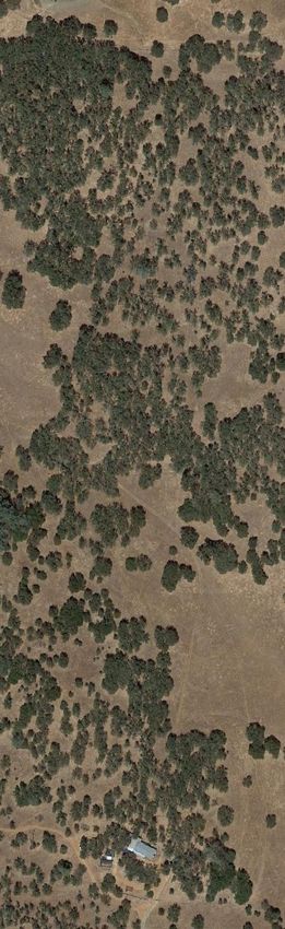
Remote Sens. 2020, 12, 2925                                                                                       3 of 19

2. Materials and Methods

2.1. Study Site
      The study site is an oak woodland savanna located in the lower foothills of the Sierra Nevada
Mountains (Tonzi Ranch, latitude: 38.431◦ N; longitude: 120.966◦ W; altitude: 177 m; average slope: 1.5◦ ).
It has a Mediterranean climate alternating between mild, wet winters and hot, dry summers.
Ninety percent of the overstory are Blue Oak (Quercus douglasii—QUDO), the remaining 10% being
mostly Grey Pine (Pinus sabiniana—PISA). Blue oaks are deciduous, their leaves start to sprout in April
and have been shed by November. The mean canopy cover (CC) of the site is 47%, and the mean LAI
is 0.8. The understory is composed of cool season annual C3 grass species active from December to
May and dry during summer and autumn. Both oak trees and grasses are active in April and May.
The soil is an Auburn very rocky silt loam (Lithic haploxerepts). More detailed site information can be
found in previous studies [25–27].
      As PISA only represent 10% of the overstory, the present study Gap Fraction plots contained either
only QUDO or a QUDO-PISA mix with a QUDO majority (Section 2.2.1). Leaf collection for EWT,
LMA and leaf pigment content estimation were done in a pure-QUDO part of the site (Section 2.2.2).
Only QUDO were modeled in the RTM, as correctly modeling coniferous trees in 3D RTMs can be
challenging [28] and no PISA-dominant plots were included in the study (three stands are mixed and
PISA canopy cover represents only 37% of the total canopy cover in the most mixed stand).
      Figure 1 shows an aerial view of the site and the locations of the various plots used in this study.
Picture of both QUDO and PISA as well as average dimensions of QUDO are shown in Figure 2a,b.

                                                                                                              4256000N

                                                                                                              4256000N

                                          677200E             677600E            678000E            678400E
                               WGS 84 / UTM Zone 10N

                                    Leaf collection trees
                                    Gap677200E
                                         Fraction plots (60x60677600E
                                                               m²)               678000E            678400E
                               WGS 84 / UTM Zone 10N

      Figure 1. Aerial view (right) of the study site and zoom-in on the leaf collection trees (left).
      Different Gap Fraction plots and leaf collection trees are identified with different colors.

                                                                         5.8 m

                                                                                            7.5 m

                                                                                   0.26 m   1.9 m

                                    (a)                                       (b)
      Figure 2. Panel (a), a picture of both a Blue Oak (foreground) and a Grey Pine (background). Panel (b),
      average dimensions of Blue Oaks at Tonzi Ranch.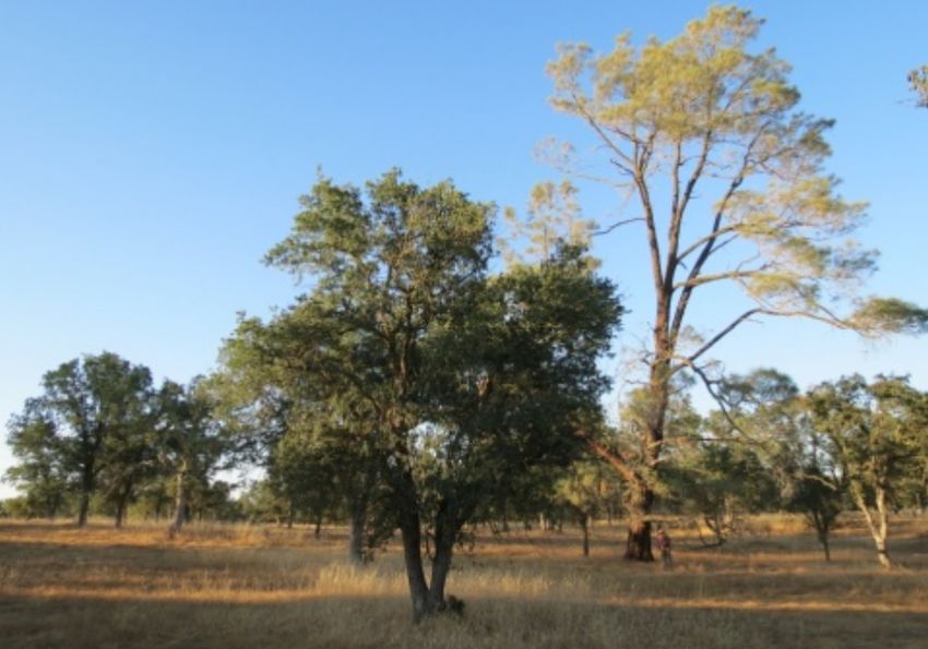
Remote Sens. 2020, 12, 2925                                                                                    4 of 19

2.2. Field Data

2.2.1. Gap Fraction
      Field data were collected coincident with the NASA Hyperspectral Infrared Imager (HyspIRI)
Mission Study Airborne Campaigns that took place in September 2013 and June 2014 and 2016
(https://hyspiri.jpl.nasa.gov/). Several digital hemispherical photographs (DHP) were collected over
multiple 60 m × 60 m plots across the study site covering all vegetation cover fractions and species
composition. These plots were selected to span the full variation in species composition and canopy
density. Information concerning the number of plots for each date is given in Table 1.
      From each 60 m × 60 m plot, nine DHP were taken using a Nikon Coolpix 4300 camera post
sunset when no direct sunlight was visible. The DHP were taken according to the sampling patterns
shown in Figure 3. DHP were processed using CAN-EYE (https://www6.paca.inrae.fr/can-eye).
CAN-EYE calculated the Gap Fraction with azimutal and zenithal resolutions of 2.5◦ , using a circle of
interest of 65◦ . The theory behind CAN-EYE estimations is described by Weiss et al. [29] and is also
available at https://www6.paca.inrae.fr/can-eye/Documentation/Documentation. As the LAI of the
site is very low, there is no significant risk of Gap Fraction saturation as this phenomenon happens for
LAI higher than 5.
                                              fresh weight − dry weight
                                     EWT =                                                           (1)
                                                       leaf area
                                                         dry weight
                                               LMA =                                                               (2)
                                                          leaf area

                              20 m

      Figure 3. Possible sampling patterns of the Gap Fraction plots. For each plot, three digital hemispherical
      photographs (DHP) (black dots) were taken in a North–South East–Southwest pattern 10 m apart in
      each of the three randomly selected 20 m × 20 m subplots (shaded in gray).

      Table 1. Field data used in this study for Gap Fraction and leaf biochemistry and associated dates of
      collection. In bold, data used for validation in the present study.

                                                               Field Data
                                       Date          Gap Fraction     Biochemistry
                                                        Plots             Trees
                                    June 2013                               3
                                 September 2013            2                5
                                   April 2014                               5
                                    June 2014              8                5
                                  October 2014                              5
                                    June 2016              7
                                 Validation data          17                13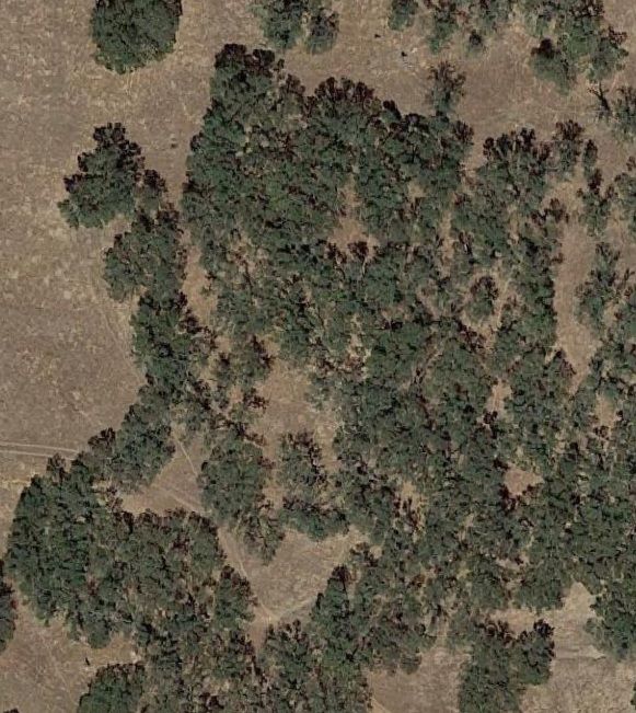
Remote Sens. 2020, 12, 2925                                                                        5 of 19

2.2.2. Equivalent Water Thickness, Leaf Mass Per Area, and Leaf Biochemistry Measurements
      To retrieve EWT, LMA, and leaf biochemistry, a set of fully expanded leaves was collected five
healthy QUDO individuals presenting a structure typical of the site. Leaves were collected from
the upper, sunlit portion of the canopy. Sampling started within an hour of the timing of the overflight.
Leaf samples were collected from open grown trees that were in full sunlight, as high into the canopy
as possible, and from branches on the east and west sides of the tree. Attention was paid to ensure
that collected leaves were healthy, and collection always occurred during dry days. Leaves were
placed in a plastic bag and stored on blue ice (or in a lab refrigerator) until lab measurements could be
made (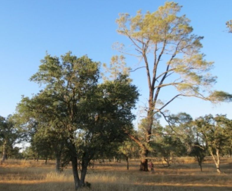
Remote Sens. 2020, 12, 2925                                                                                                    6 of 19

2.3. PROSAIL2DART

2.3.1. Methodology
     Both PROSAIL and DART were used to compute scene reflectances over a calibration (LAI, Cab ,
                                                                                   ρ
Car, LMA, EWT) grid hereafter designated as cal. Band reflectance ratios ρ DART were computed for
                                                                                  PROSAIL
each point of the grid and used to calibrate linear 5-D interpolators. These interpolators are used to
transform any reflectance obtained with PROSAIL into a reflectance similar to what DART would
have obtained. For each date, one 5-D interpolator was computed for each (CC, understory reflectance,
Anthocyanins content (Cant )) triplet as these parameters were either not possible to model in PROSAIL
(CC) or to limit the uncertainties (understory reflectance, Cant ). This calibration/transformation method
is hereafter called PROSAIL2DART (P2D). A diagram of the methodology is shown in Figure 4.

                                                           PROSAIL2DART

                   PROSAIL reflectance                                                                     corresponding
                   spectra at arbitrary                       transformation                              DART-approximated
                   (LAI, Cab, Car, LMA, EWT)                                                              reflectance spectra

                                                                         transformation ratios at any
                                                                         location within cal boundaries

                                                              Generalization

                                                                         reflectance ratios with
                                                                         a discrete sampling

                                                    for every (LAI, Cab, Car, LMA, EWT)
                   DART and PROSAIL                 of the cal grid:
                   reflectance spectra ρ
                   over the calibration
                   grid cal

                                               Figure 4. PROSAIL2DART methodology.

2.3.2. RTM Parametrization

DART
     DART version 5.7.3v1078 was used to simulate canopy reflectances. DART is a radiation
transfer model able to simulate light interactions and multiple scattering effects within a
3D scene, including the topography and the atmosphere. DART includes PROSPECT to
model leaf reflectance and transmittance. A precise description of the DART model can
be found in Gastellu-Etchegorry et al. [32] and Gastellu-Etchegorry et al. [23]. Trees are defined by
structural parameters such as the shape and size of their crown or the distribution and optical properties
of their leaves.
     The scene modeling done in this study is based on the same simplified forest representation as
the one done in Miraglio et al. [30]: canopy is represented with 4 lollipop trees and the ground is
modeled as a lambertian surface, the reflectance of which was extracted from AVIRIS-C images, as this
previously proved sufficient to estimate both LAI and leaf pigment content at the AVIRIS-C spatial
resolution. Different soil reflectance were considered: from the sets of pure soil pixels extracted from
open parts of the site, mean and mean ± standard deviation reflectances were used to build the LUTs
in order to better take into account possible ground reflectance variations over the site. For simplicity
purposes and to ensure that (i) the (LAI, Cab , Car, LMA, EWT) space that could be covered by P2D was
an hyperrectangle and (ii) the density of calibration samples was uniform over this space, cal followed
a regular sampling scheme. Tables 3 and 4 describe the various inputs used to create the DART scenes.
     The Gap Fractions of the DART scenes were computed for all combinations of CC and LAI.
It was retrieved using the DART 3D Radiative Budget tool, by considering the percentage of diffuse
illumination intercepted by the ground. The specific DART parameters to obtain these results are
Remote Sens. 2020, 12, 2925 7 of 19
• illumination using a single wavelength,
• no radiative transfer in the atmosphere,
• SKYL (atmospheric scattering of sun radiance) set to 1,
• number of iterations set to 0, and
• smaller mesh size of irradiance sources set to 0.005 m
Gap Fraction can be considered a function of CC an LAI, i.e., Gap Fraction = f (CC, LAI).
Therefore, when generating the P2D, fine LUTs Gap Fractions were derived from the (CC, LAI) values
by linear interpolation, using the test and cal values as reference.
Table 3. DART-fixed scene parameters used in this study for the calibration and test Look-Up Tables
(LUTs). PROSAIL used the same LAD and sun zenith/azimuth as DART.
Parameter Value
Voxel size x, y, z (m) 0.4, 0.4, 0.4
Tree height (m) 9.4
Crown shape ellipsoidal
Crown diameter (m) 5.8
Crown height (m) 7.5
Trunk height (m) 6.63
Trunk dbh (m) 0.26
LAD spherical
Sun zenith/azimut according to acquisition date
Table 4. DART, PROSAIL, and PROSPECT variable parameters used for the calibration (cal) and test
(test) LUTs. For Cant , values between parentheses concern the September 2013 LUT, other values
concern all June LUTs.
Values/Range Step
Parameter cal test cal test
CC (%) 10–90 10–90 20
LAI (m2 /m2 ) 0.1–1.9 0.25–1.75 0.3
Cab (µg/cm2 ) 10–60 15–55 10
Car (µg/cm2 ) 2–14 4–12 4
LMA (g/cm2 ) 7–16 × 10−3 8.5–14.5 × 10⁻³ 3× 10⁻³
EWT (cm) 5–17 × 10−3 7–15 × 10−3 4 × 10⁻³
Cant (µg/cm2 ) 0(0–2) 0 0(2) 0
Ground Reflec. mean, mean ± Std June 2016 mean
PROSAIL
The 4SAIL version of PROSAIL was used in the present study, using a Python wrapper (https:
//github.com/jgomezdans/prosail, DOI: 10.5281/zenodo.2574925). PROSAIL combines the leaf
model PROSPECT with the 1-D turbid canopy RTM SAIL. A thorough description and history of the
PROSAIL model can be found in Berger et al. [33]. Leaf angle distribution (LAD) is not a direct input of
PROSAIL and both the average leaf slope LIDFa and the associated distribution bimodality LIDFb must
be given. A spherical LAD is obtained with LIDFa = −0.35 and LIDFb = −0.15. Ground reflectance was
the same reflectance as that given to DART, as were the solar zenith and azimuth angles. LAI variations
were the same as those given to DART.
PROSPECT
Leaf optical properties were simulated using the PROSPECT model, which is implemented in
DART and PROSAIL. PROSPECT-D [34] was used in this study, and a small Cant was introduced as a
possible case for September to take into account possible leaf senescence. The leaf structure parameter
N was set to 1.8. The PROSPECT specific parameters considered in this study are given in Table 4.Remote Sens. 2020, 12, 2925 8 of 19
2.3.3. Error Assessment
As the P2D linear interpolators were calibrated on a regular grid, the maximum differences
between P2D and DART reflectances are located at the centers of the hypercubes defined by the cal
grid. The P2D approach will be validated if the difference between P2D and DART reflectances at the
hypercube center are negligible.
Let test designate the set of the hypercubes centers, which correspond to the test grid.
Let P2D test and D test be the reflectances computed by P2D and DART on test points and D cal the
reflectances computed by DART on cal points, which correspond to the hypercubes corners. The P2D
approximation was evaluated using the E ratio, computed as
P2Ditest − Ditest
E = median × 100 (3)
i min Ditest − Di,j
cal
j >0.001
with i the hypercube identifier and j the hypercube corner identifier. This ratio was designed to
compare the reflectance distance between P2D and DART at the hypercube center (maximum error)
with the reflectance distance between the hypercube center and corners obtained through DART.
A value close to 100 indicates that the P2D error is similar to the smallest difference between the
hypercube’s center and corners, while a value close to 0 indicates that the P2D error is negligible.
An illustration of the P2D validation methodology is presented Figure 5. An E value lower than
50 indicates that the P2D approximation is closer to the hypercube center than the corners. A condition
that Ditest − Di,j
cal should be non-negligible (>0.001 when reflectance range is 0 to 1) was used as
variables do not necessarily have an influence at all wavelengths, which could lead to close to zero
differences between some corners and the center and make E diverge erroneously.
Reflectance absolute
difference
LAI- LAI+
EWT- LAI
EWT+
EWT
|Dtest - Dcal |>0.001 |Dtest - Dcal |≤0.001
min |Dtest - Dcal |>0.001
|Dtest - P2Dtest |
LAI+ hypercube i corners
Figure 5. Illustration of the P2D validation methodology on a 2D grid, with calculation of the various
differences necessary to compute E for one hypercube.
2.4. Fine Lut Building
P2D was subsequently used to generate a fine DART-like LUT for each AVIRIS-C image, following
a Latin Hypercube sampling. The correlation between Cab and Car visible in the field data was takenRemote Sens. 2020, 12, 2925 9 of 19
into account by constraining the Car values around 2.5 times the standard deviation between field
data and the regression line (see Figure 6). For LAI, Cab , LMA and EWT are the boundaries of the
Latin Hypercube corresponding to those of the calibration LUTs presented in Table 4. Only CC 30 to
90% were considered, and for every ground reflectance and Cant value, 50,000 cases were generated
and distributed equally among the CC. Therefore, June 2013, 2014, and 2016 fine LUTs each have
150,000 entries, and September 2013 LUT has 300,000 entries.
Figure 6. Relationship between Car and Cab in the field data (dots) and as implemented (shaded area)
with the Latin Hypercube sampling.
2.5. Lut-Based Inversions
To assess the performance improvement when using P2D instead of simply using DART with a
regular sampling scheme, both DART cal and P2D fine LUTs were used to retrieve Gap Fraction and
leaf biochemistry. LUT-based approaches consist in finding the simulated reflectance ŷ that is the most
similar to the measured one, y, according to a cost function. Several cost functions were selected for
this study: root mean square error (RMSE; Equation (4)), spectral angle mapper (SAM; Equation (5)),
and vegetation index (VI) differences (DV I ; Equation (6)).
r
1 N
RMSE(y, ŷ) = Σ (y − ŷi )2 (4)
N i =1 i
−1 q ΣiN=1 yi ŷi
SAM(y, ŷ) = cos q (5)
ΣiN=1 ŷi ŷi ΣiN=1 yi yi
DV I (y, ŷ) = abs (V I (y) − V I (ŷ)) (6)
RMSE and SAM were computed using variable-specific spectral intervals. The Gap Fraction
interval covered the near-infrared (NIR) and short wavelength infrared (SWIR) (INT GAP, 0.8–2.45 µm).
Intervals for Cab and Car were parts of the visible range (INT CAB, 0.5–0.75; INT CAR, 0.5–0.55 µm),
while those used for LMA and EWT were parts of the NIR and SWIR (INT LMA, 0.8–1.3; INT EWT,
1.3–2.45 µm). The spectral intervals were chosen based on their sensitivity to the variables of interest
according to the results of a Sobol sensitivity analysis on the DART cal LUTs (not shown).
Before LUT-based inversion, VI capabilities to estimate the variables of interest were assessed by
fitting a function between VI and variables (V I = v a + b for biochemistry and V I = a × v + b for Gap
Fraction, with v the variable’s value). If no relationship could be found, the VI was not considered for
the inversion.Remote Sens. 2020, 12, 2925 10 of 19
Table 5 shows all the cost functions tested for this study for each variable of interest, as well as
the goodness of the fit of each VI when applicable. Estimation results were computed as the mean of
multiple best solutions. The number of solutions considered for each LUT was 0.5% of the LUT size.
Table 5. Cost functions used in this study, best R2 obtained across all LUTs for the vegetation index
(VI) and associated performances for the LUT-based (DART and P2D) inversions (when applicable).
dr
VI Source VI R2
DART cal P2D fine LUT
Gap fraction
RMSE INT GAP 0.75 0.75
SAM INT GAP 0.76 0.76
D NDV I Tucker [35] 0.96 0.78 0.77
D MSAV I2 Qi et al. [36] 0.9 0.76 0.74
Cab
RMSE INT CAB 0.49 0.31
SAM INT CAB 0.12 0.23
DTCARI/OSAV I Haboudane et al. [37] 0.81 0.25 0.23
D Maccioni Maccioni et al. [38] 0.91 0.57 0.69
DgNDV I Smith et al. [39] 0.76 0.65 0.75
DGM_94b Gitelson and Merzlyak [40] 0.6 0.65 0.77
D MCARI2 Haboudane et al. [41] 0.01
Car
RMSE INT CAR −0.08 0.2
SAM INT CAR −0.37 0.53
DR515_R570 Hernández-Clemente et al. [22] 0.29
DCRI550 Gitelson et al. [42] 0.09
DTCARI/OSAV I Haboudane et al. [37] 0.72 0.04 0.27
D Maccioni Maccioni et al. [38] 0.81 0.12 0.59
DgNDV I Smith et al. [39] 0.68 0.11 0.64
DGM_94b Gitelson and Merzlyak [40] 0.61 0.34 0.65
D MCARI2 Haboudane et al. [41] 0.01
LMA
RMSE INT LMA 0.03 0.19
SAM INT LMA 0.29 0.24
Dlma_ND le Maire et al. [43] 0
Dlma_D le Maire et al. [43] 0.5 −0.34 0.1
D NDN I Serrano et al. [44] 0
D NDLI Serrano et al. [44] 0
EWT
RMSE INT EWT −0.32 0.04
SAM INT EWT −0.49 0.29
DEV I Huete et al. [45] 0
D NDW I Gao [46] 0.01
DSIWSI Fensholt and Sandholt [47] 0.02
D NDI7 Trombetti et al. [48] 0.01
D NDI I Hardisky et al. [49] 0
DSRW I Zarco-Tejada et al. [50] 0.01
D MSI Hunt and Rock [51] 0
DSW IRR Trombetti et al. [48] 0.01
DW I Penuelas et al. [52] 0.01Remote Sens. 2020, 12, 2925 11 of 19
2.6. Validation Metrics
Gap fraction, leaf pigments content, EWT, and LMA estimates were compared with the field
measurements available using the following criteria; total RMSE, systematic and unsystematic RMSE
(Willmott [53]), the model performance index dr (Willmott et al. [54]), and R2 of the predicted vs.
measured regression line.
Concerning Gap Fraction, each validation point was the average of Gap Fraction values derived
from hemispherical pictures taken within a 60 m × 60 m plot (see Section 2.2.1). Direct comparison
between pixel-estimated value and validation data can be inappropriate as the area covered by the
DHP of a plot is wider than the AVIRIS-C pixel (18 m × 18 m). Therefore, validation values were
compared to the average of the Gap Fractions estimated over a 3 × 3 pixels windows centered on the
pixel corresponding to the plot center, similarly to the method employed in Miraglio et al. [30].
Biochemistry validation data were obtained at the leaf scale, for one tree in each validation pixel.
It was assumed that biochemistry estimations could be directly extracted from the pixels associated
with the acquisition positions.
3. Results
3.1. Comparison between Aviris-C and Dart Reflectances
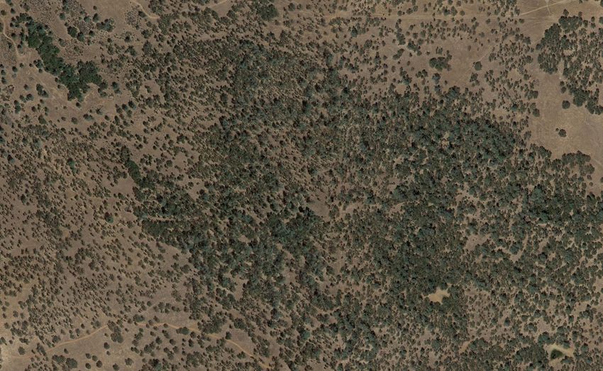
Figure 7 shows the validation pixels’ reflectances and compares them to the reflectance extrema
found in their corresponding LUT. For June 2013, September 2013 and June 2016, all pure pixel
reflectances fall within the extrema of the LUTs whatever the wavelength. One reflectance from a
mixed plot is severely out of the boundaries of the LUT, while up to 8 other mixed plot reflectances
are slightly below the LUT minima between 0.9 and 1.6 µm, for a total of at most 9 reflectances below
the LUT minima at some wavelengths out of 63 for June 2016. For June 2014, almost all reflectances
including those from mixed pixels also fall within the extrema: of the 68 pixel reflectances, 6 are below
the LUT minima around 1.24 µm and 1.6 µm, with a maximum difference of 0.02.
Figure 7. LUT reflectances and AVIRIS-C reflectances at validation pixels for each date (from left
to right: June 2013, September 2013, June 2014, June 2016). In red, reflectance boundaries of the
associated LUT, in gray, AVIRIS-C reflectances. In blue, AVIRIS-C reflectances from mixed QUDO-PISA
validation pixels.
3.2. PROSAIL2DART Errors
Figure 8 and Table 6 show the evolution of the E ratio over the CC and wavelengths. In the visible,
all wavelengths are well approximated by P2D for CC ≥ 30%, with the highest E value being 21% at
0.68 µm and 30% CC. While for 10% CC, the green and NIR are also well approximated (E < 50%),
this is not the case for the blue and red regions where E can be above 50%. In the SWIR, for 10% CC
E values are considerably below 50% for λ < 1.8 µm. However, higher values are found at higher
wavelengths and the maximum, 46%, is obtained at 1.49 µm. Estimations with either DART cal or P2D
LUTs only used the CC ≥ 30% cases to avoid uncertainties.Remote Sens. 2020, 12, 2925 12 of 19
100
10
10
80
30
30
60
E (%)
CC
50
CC
50
40
70
70
20
90
90
0
0.8
0.9
1.0
1.1
1.2
1.3
1.4
1.5
1.6
1.7
1.8
1.9
2.0
2.11
2.21
2.31
2.41
0.46 0.57 0.68 0.79
Wavelength ( m) Wavelength ( m)
(a) (b)
Figure 8. P2D error for each wavelength and CC over the (a) visible and (b) near-infrared (NIR) spectral
regions. Panels (a,b) share the same color bar.
Table 6. Maximum value of the E ratio and associated wavelength for each CC over the visible (VIS)
and NIR spectral ranges.
Maximum E (%) Wavelength (µm)
CC
VIS NIR VIS NIR
10 87 46 0.68 1.49
30 21 21 0.68 2.45
50 9 13 0.73 1.13
70 8 10 0.73 1.10
90 6 8 0.76 0.88
3.3. PROSAIL2DART Fine Lut Generation
It took 12,666 h (total CPU time of a server equipped with Broadwell Intel R Xeon R CPU E5-2650
v4 @ 2.20 GHz) to generate the 21,840 reflectances required to build the DART cal LUT dedicated
to September 2013 (the most extensive LUT, as two values of anthocyanins are also considered).
For comparison, once P2D was calibrated (the calibration time is negligible), it took 1.5 h (total CPU
time on a computer equipped with an Intel R CoreTM i5-6300HQ CPU @ 2.30 GHz) to generate the
300,000 entries of the P2D fine LUT.
3.4. Estimation Performances
Table 5 shows the best R2 achieved by the various VI when fitted over each LUT. Gap Fraction
was very well measured by its VI, and overall so were Cab and Car, with only MCARI2, R515_570,
and CRI550 presenting no relation with the estimates’ values. Concerning LMA and EWT, no satisfying
relation could be found, and only lma_D could find a slight relation with a R2 of 0.5. Only the inversion
methods with R2 higher than 0.5 were considered suitable candidates for LUT-based inversions.
Concerning Gap Fraction, both LUTs perform in equivalent manner, with good performances
whatever the method (maximum dr is 0.78 for D NDV I applied on DART cal and 0.77 when applied on
the P2D LUT). Cab estimations show improved performances with the P2D LUTs for all cost functions
except RMSE INT CAB and DTCARI/OSAV I , which have slightly lower dr . DGM_94b offers the best
performances, with dr = 0.77 when applied on the P2D LUTs. For Car, the best dr is also obtained
with the P2D LUTs with DGM_94b , and P2D consistently improved the dr . Concerning LMA and
EWT, the P2D fine LUTs appear to slightly improve performances for the selected cost functions
(at the exception of SAM INT LMA that decreases slightly); however, dr remains low. Their respective
best-performing cost functions are SAM INT LMA with DART cal and SAM INT EWT with P2D.Remote Sens. 2020, 12, 2925 13 of 19
3.5. Estimation Plots
Figure 9 compares estimated and field values for the various estimates of this study when using
the best performing methods identified in Section 3.4. Gap Fraction estimations present both a high
R2 and a low RMSE (0.78 and 0.1, respectively). While it appears that one of the June 2014 mixed
plots (yellow) was overestimated, other mixed plots present a similar behavior as pure QUDO plots.
Similar behaviors are found for Cab and Car: most of the points seem to follow the first bisector, and the
point with the highest Cab and Car values is slightly underestimated. RMSE errors in both cases remain
low (4.14 and 1.05 µg/cm2 , respectively). No trend between estimations and field data could be found
for either LMA and EWT (their respective R2 are 0.14 and 0.01) and RMSE of 2.2 × 10⁻³ g/cm2 and
2 × 10⁻³ cm are obtained.
(a) (b) (c)
(d) (e)
Figure 9. Comparison between estimated and measured parameters using the best-performing methods
identified in Table 5. Panels (b–e) were obtained with the P2D fine LUTs, and panels (a,d) were obtained
with the DART calibration LUTs. Marker color identifies the location within the study site, and for Gap
Fraction QUDO-PISA mixed stands are identified with bicolored markers.
4. Discussion
4.1. PROSAIL2DART Performances
Choosing a sampling method for the variables’ space for LUT generation, either for LUT-based
inversions or calibration of machine-learning methods, is a critical step. No ideal sampling has yet be
determined: Darvishzadeh et al. [55] and Hernández-Clemente et al. [22] used uniform distributions
over the variables’ intervals; Malenovsky et al. [56] and Leonenko et al. [57] considered a regular grid
for LAI; and Richter et al. [58] and Verrelst et al. [59] used both uniform and Gaussian distribution
for the parameters of interest. These methods can lead to different estimation accuracies, as they may
put an emphasis on unadapted ranges or allow for the existence of duplicate or near-duplicate cases.
However, as LUT-building is very time-consuming when using 3D RTMs, it is difficult to test different
sampling methods.
As shown in Figure 5, the intrinsic error of the P2D approximation is very low for all wavelengths
at CC 30% and gets lower when the CC increases, as the higher the CC the closer a DART scene is
to a completely turbid medium. The error E calculated in this study is also relative to the cal LUT’s
sampling, so lower absolute errors could be obtained by simply refining the calibration sampling.Remote Sens. 2020, 12, 2925 14 of 19
This low intrinsic error made it possible to approximate with minimal error DART outputs using the
PROSAIL model, which has considerably shorter computation times. Each interpolator necessitated
a total of 784 (672 in the visible and 112 in the NIR and SWIR) DART reflectances. As specified in
Section 3.3, the most extensive calibration LUT, encompassing 21,840 cases, necessitated 12,666 CPU
hours to generate with DART 5.7.3v1078 and allowed for calculating 300,000 entries in 1.5 h, which is a
significant decrease of the computation time. Even though the latest DART versions are significantly
faster than the version used in this study, the execution time remains considerably longer than P2D as
P2D is basically as fast as PROSAIL.
This short execution time makes it possible to test various sampling schemes and either use the
output reflectances as is, as the P2D error is small, or determine an optimal sampling scheme to use for
final LUT generation with the 3D RTM.
4.2. Gap Fraction Estimations
Table 5 and Figure 9a show that Gap Fraction estimations are good, with high dr and low RMSE,
and that this is true no matter the estimation strategy. Indeed, all methods presented a dr higher than
0.7, a RMSE lower than 0.11, and a R2 higher than 0.73 (not shown), and using the P2D LUTs did
not lead to significant improvement of the estimations. The method presenting the highest dr was
D NDV I . When estimating scene LAI over the site, Miraglio et al. [30] also identified this method as the
best performing. The LAI had been obtained from the same DHP pictures, with the assumption that
effective plant area index (PAI) was equivalent to true LAI [60]. As effective PAI is derived from the
DHP Gap Fraction, the fact that the same inversion strategy yielded good estimation results for both
Gap Fraction and true LAI may confirm that true LAI can be considered equivalent to effective PAI for
sparse broad-leaved forests.
4.3. Pigment Estimations
Cab and Car estimations (RMSE 4.14 and 1.85 µg/cm2 and R2 of 0.73 and 0.52, respectively) are in
line with what can be found in the literature: Zarco-Tejada et al. [61] obtained a RMSE of 8.1 µg/cm2
for Cab over open-canopy tree crops; le Maire et al. [43] obtained a RMSE of 8.2 µg/cm2 estimating
leaf Cab of broadleaved forests; Darvishzadeh et al. [62] had an RMSE of 8.6 µg/cm2 when estimating
leaf Cab of spruce stands; Zarco-Tejada et al. [63] obtained a 1.3 µg/cm2 RMSE for Car estimation in
vineyards with high-resolution imagery; Huang et al. [64] had a 2.02 µg/cm2 RMSE when monitoring
crop Car.
While final Cab estimation performances obtained in this study are similar or better than those
obtained by Miraglio et al. [30], there are two main differences between the two methodologies:
The first one is that the previous study used PROSPECT-5 and not PROSPECT-D: the principal
differences between PROSPECT-D and -5 are the introduction of anthocyanins and the modification
of the pigments specific absorption coefficients (SAC) at various wavelengths [34]: the chlorophylls
SAC were lowered over the 0.45–0.65 µm interval and increased over 0.65–0.7 µm, and the carotenoids
SAC were increased over the 0.45–0.55 µm interval. The second difference is the sampling scheme,
which was previously a regular grid over the variables’ variation ranges, meaning that no correlation
between Cab and Car, such as the one visible Figure 6, could be modeled. While this was not critical for
Cab estimations, as the high dr values in Table 5 show, this limited the number of possible VI to use for
Car estimations. Introducing the relationship between Cab and Car when building the LUTs allowed
to use Cab VI for Car estimations, which proved to be more adequate. This relationship also helps to
reduce the unnecessary cases in the LUTs, as low Cab -high Car cases (and vice versa) are unrealistic
and could bring confusion when doing the inversions.Remote Sens. 2020, 12, 2925 15 of 19
4.4. LMA and EWT Estimations
The RMSE obtained for LMA was 0.0022 g/cm2 , more than two times higher than the
9.1 × 10⁻⁴ g/cm2 value obtained by le Maire et al. [43] over a higher LAI broadleaved forest.
EWT estimations present a 0.002 cm RMSE. Neither LMA nor EWT present good R2 . As visible
in Table 5, almost none of the VI tested for these variables showed a relationship with them. This is in
line with the results found by Yanfang Xiao et al. [65], who showed using PROSAIL that for LAI lower
than 3 it was not possible to estimate EWT as its contribution to the signal was too low in comparison
to LAI’s and ground’s. It is possible that higher resolution hyperspectral images would be needed for
EWT and LMA estimation, as this would make it possible to locate pure-vegetation pixels where EWT
and LMA spectral signature would be more visible.
5. Conclusions
The results obtained in this study demonstrated the possibility to approximate with minimal
error the reflectance outputs of DART with those of PROSAIL even at low (30%) CC. For higher CC,
it was shown that approximation errors were negligible. The approximation model was further used
to generate extensive LUTs to estimate Gap Fraction of mixed oak and pine stands as well as leaf
Cab , Car, EWT, and LMA of oak stands in a low-foliage woodland savanna. Gap Fraction and leaf
pigment content estimations presented similar or improved performances when taking advantage of
the proposed model instead of only relying on DART. EWT and LMA could not be retrieved using
either models.
In summary, the findings show that acceptably approximating DART results from PROSAIL is
possible and that the subsequent reflectances can be successfully used for estimation purposes of even
very sparse oak stands, although conclusions should also applicable to other broadleaved stands due
to the elementary modeling used in the 3D RTM. This is valuable, as 1D RTMs are dramatically faster
than 3D RTMs. In the exploration phase, this allows for the testing of various sampling schemes at
a negligible cost for either the training of machine learning methods, that require extensive training
databases, or the generation of more complex LUTs. Approximated reflectances can also directly be
used as is to retrieve canopy structural and biochemical parameters with acceptable accuracy.
Due to the tree distribution within the study site and the ground sampling distance of AVIRIS-C,
no pine-dominant stands could be considered for Gap Fraction and leaf biochemistry estimations
and this study focused mainly on pure-oak stands. Further work is necessary to extend them to
coniferous trees or mixed stands. More work is also necessary to acceptably estimate EWT and LMA
of tree–grass ecosystems, possibly by improving the soil realism by modeling the grass layer [66] or
the tree representation with the inclusion of detailed trunk structures [16] within the 3D RTM.
Author Contributions: Conceptualization, T.M., S.U. and X.B.; Data curation, T.M., K.A. and M.H.;
Formal analysis, T.M.; Funding acquisition, K.A., S.U. and X.B.; Investigation, T.M.; Methodology, T.M. and
X.B.; Project administration, S.U. and X.B.; Resources, K.A., M.H. and S.U.; Software, T.M.; Supervision, S.U. and
X.B.; Validation, T.M.; Visualization, T.M.; Writing—original draft, T.M. and M.H.; Writing—review and editing,
K.A., M.H., S.U. and X.B. All authors have read and agreed to the published version of the manuscript.
Funding: This research was funded by the Office Nationale d’Études et de Recherches Aérospatiales (ONERA)
and by Région Occitanie.
Acknowledgments: The authors are grateful to the CSTARS team for collecting and processing the field data,
and to NASA JPL from providing AVIRIS-C data (NASA grant No. NNX12AP08G). They also thank Jean-Philippe
Gastellu-Etchegorry from CESBIO for his insight and help concerning the DART simulations.
Conflicts of Interest: The authors declare no conflicts of interest. The funders had no role in the design of the
study; in the collection, analyses, or interpretation of data; in the writing of the manuscript; or in the decision to
publish the results.Remote Sens. 2020, 12, 2925 16 of 19
References
1. Pereira, H.M.; Ferrier, S.; Walters, M.; Geller, G.N.; Jongman, R.H.; Scholes, R.J.; Bruford, M.W.; Brummitt, N.;
Butchart, S.H.; Cardoso, A.C.; et al. Essential biodiversity variables. Science 2013, 339, 277–278. [CrossRef]
[PubMed]
2. Paz-Kagan, T.; Asner, G.P. Drivers of woody canopy water content responses to drought in a
Mediterranean-type ecosystem. Ecol. Appl. 2017, 27, 2220–2233. [CrossRef] [PubMed]
3. Féret, J.B.; le Maire, G.; Jay, S.; Berveiller, D.; Bendoula, R.; Hmimina, G.; Cheraiet, A.; Oliveira, J.C.;
Ponzoni, F.J.; Solanki, T.; et al. Estimating leaf mass per area and equivalent water thickness based on leaf
optical properties: Potential and limitations of physical modeling and machine learning. Remote Sens. Environ.
2018, 231, 110959. [CrossRef]
4. Jetz, W.; McGeoch, M.A.; Guralnick, R.; Ferrier, S.; Beck, J.; Costello, M.J.; Fernandez, M.; Geller, G.N.;
Keil, P.; Merow, C.; et al. Essential biodiversity variables for mapping and monitoring species populations.
Nat. Ecol. Evol. 2019, 3, 539–551. [CrossRef]
5. Xu, L.; Baldocchi, D.D. Seasonal trends in photosynthetic parameters and stomatal conductance of blue oak
(Quercus douglasii) under prolonged summer drought and high temperature. Tree Physiol. 2003, 23, 865–877.
[CrossRef]
6. Krinner, G.; Viovy, N.; de Noblet-Ducoudré, N.; Ogée, J.; Polcher, J.; Friedlingstein, P.; Ciais, P.; Sitch, S.;
Prentice, I.C. A dynamic global vegetation model for studies of the coupled atmosphere-biosphere system.
Glob. Biogeochem. Cycles 2005, 19, 1–33. [CrossRef]
7. Ma, S.; Baldocchi, D.D.; Mambelli, S.; Dawson, T.E. Are temporal variations of leaf traits responsible for
seasonal and inter-annual variability in ecosystem CO2 exchange? Funct. Ecol. 2011, 25, 258–270. [CrossRef]
8. Ustin, S.L.; Roberts, D.A.; Gamon, J.A.; Asner, G.P.; Green, R.O. Using Imaging Spectroscopy to Study
Ecosystem Processes and Properties. BioScience 2004, 54, 523. [CrossRef]
9. Cheng, Y.B.; Zarco-Tejada, P.J.; Riaño, D.; Rueda, C.A.; Ustin, S.L. Estimating vegetation water content
with hyperspectral data for different canopy scenarios: Relationships between AVIRIS and MODIS indexes.
Remote Sens. Environ. 2006. [CrossRef]
10. Zarco-Tejada, P.J.; Hornero, A.; Beck, P.S.; Kattenborn, T.; Kempeneers, P.; Hernández-Clemente, R.
Chlorophyll content estimation in an open-canopy conifer forest with Sentinel-2A and hyperspectral imagery
in the context of forest decline. Remote Sens. Environ. 2019, 223, 320–335. [CrossRef]
11. Baret, F.; Buis, S. Estimating Canopy Characteristics from Remote Sensing Observations: Review of Methods
and Associated Problems. In Advances in Land Remote Sensing: System, Modeling, Inversion and Application;
Liang, S., Ed.; Springer: Dordrecht, The Netherlands, 2008; pp. 173–201. [CrossRef]
12. Verrelst, J.; Camps-Valls, G.; Muñoz-Marí, J.; Rivera, J.P.; Veroustraete, F.; Clevers, J.G.; Moreno, J.
Optical remote sensing and the retrieval of terrestrial vegetation bio-geophysical properties—A review.
ISPRS J. Photogramm. Remote Sens. 2015, 108, 273–290. [CrossRef]
13. Pinty, B.; Gobron, N.; Widlowski, J.L.; Gerstl, S.A.; Verstraete, M.M.; Antunes, M.; Bacour, C.; Gascon, F.;
Gastellu, J.P.; Goel, N.; et al. Radiation transfer model intercomparison (RAMI) exercise. J. Geophys.
Res. Atmos. 2001, 106, 11937–11956. [CrossRef]
14. Pinty, B.; Widlowski, J.L.; Taberner, M.; Gobron, N.; Verstraete, M.M.; Disney, M.; Gascon, F.; Gastellu, J.P.;
Jiang, L.; Kuusk, A.; et al. Radiation Transfer Model Intercomparison (RAMI) exercise: Results from the
second phase. J. Geophys. Res. Atmos. 2004, 109. [CrossRef]
15. Widlowski, J.L.; Taberner, M.; Pinty, B.; Bruniquel-Pinel, V.; Disney, M.; Fernandes, R.;
Gastellu-Etchegorry, J.P.; Gobron, N.; Kuusk, A.; Lavergne, T.; et al. Third Radiation Transfer Model
Intercomparison (RAMI) exercise: Documenting progress in canopy reflectance models. J. Geophys.
Res. Atmos. 2007, 112. [CrossRef]
16. Widlowski, J.L.; Pinty, B.; Lopatka, M.; Atzberger, C.; Buzica, D.; Chelle, M.; Disney, M.;
Gastellu-Etchegorry, J.P.; Gerboles, M.; Gobron, N.; et al. The fourth radiation transfer model intercomparison
(RAMI-IV): Proficiency testing of canopy reflectance models with ISO-13528. J. Geophys. Res. Atmos. 2013,
118, 6869–6890. [CrossRef]
17. Hanan, N.; Hill, M.J. Savannas in a Changing Earth System: The NASA Terrestrial Ecology Tree-Grass Project;
Earth Science Division: Washington, DC, USA, 2012; p. 56.Remote Sens. 2020, 12, 2925 17 of 19
18. Ali, A.M.; Darvishzadeh, R.; Skidmore, A.K.; Duren, I.V. Effects of Canopy Structural Variables on Retrieval
of Leaf Dry Matter Content and Specific Leaf Area from Remotely Sensed Data. IEEE J. Sel. Top. Appl. Earth
Obs. Remote Sens. 2016. [CrossRef]
19. Atzberger, C. Development of an invertible forest reflectance model: The INFORM-Model. In A Decade
of Trans-European Remote Sensing Cooperation, Proceedings of the 20th EARSeL Symposium, Dresden, Germany,
14–16 June 2000; Buchrointher, M.F., Ed.; CRC Press: Boca Raton, FL, USA, 2000; pp. 39–44.
20. Weiss, M.; Baret, F.; Myneni, R.B.; Pragnère, A.; Knyazikhin, Y. Investigation of a model inversion technique
to estimate canopy biophysical variables from spectral and directional reflectance data. Agronomie 2000.
[CrossRef]
21. Ali, A.M.; Skidmore, A.K.; Darvishzadeh, R.; van Duren, I.; Holzwarth, S.; Mueller, J. Retrieval of forest leaf
functional traits from HySpex imagery using radiative transfer models and continuous wavelet analysis.
ISPRS J. Photogramm. Remote Sens. 2016. [CrossRef]
22. Hernández-Clemente, R.; Navarro-Cerrillo, R.M.; Zarco-Tejada, P.J. Carotenoid content estimation
in a heterogeneous conifer forest using narrow-band indices and PROSPECT+DART simulations.
Remote Sens. Environ. 2012. [CrossRef]
23. Gastellu-Etchegorry, J.P.; Yin, T.; Lauret, N.; Cajgfinger, T.; Gregoire, T.; Grau, E.; Feret, J.B.; Lopes, M.;
Guilleux, J.; Dedieu, G.; et al. Discrete anisotropic radiative transfer (DART 5) for modeling airborne and
satellite spectroradiometer and LIDAR acquisitions of natural and urban landscapes. Remote Sens. 2015.
[CrossRef]
24. Jacquemoud, S.; Verhoef, W.; Baret, F.; Bacour, C.; Zarco-Tejada, P.J.; Asner, G.P.; François, C.; Ustin, S.L.
PROSPECT + SAIL models: A review of use for vegetation characterization. Remote Sens. Environ. 2009, 113.
[CrossRef]
25. Baldocchi, D.D.; Xu, L.; Kiang, N. How plant functional-type, weather, seasonal drought, and soil physical
properties alter water and energy fluxes of an oak-grass savanna and an annual grassland. Agric. For. Meteorol.
2004, 123, 13–39. [CrossRef]
26. Chen, Q.; Baldocchi, D.; Gong, P.; Dawson, T. Modeling radiation and photosynthesis of a heterogeneous
savanna woodland landscape with a hierarchy of model complexities. Agric. For. Meteorol.
2008, 148, 1005–1020. [CrossRef]
27. Ma, S.; Baldocchi, D.D.; Xu, L.; Hehn, T. Inter-annual variability in carbon dioxide exchange of an oak/grass
savanna and open grassland in California. Agric. For. Meteorol. 2007, 147, 157–171. [CrossRef]
28. Janoutová, R.; Homolová, L.; Malenovskỳ, Z.; Hanuš, J.; Lauret, N.; Gastellu-Etchegorry, J.P. Influence of 3D
spruce tree representation on accuracy of airborne and satellite forest reflectance simulated in DART. Forests
2019, 10, 292. [CrossRef]
29. Weiss, M.; Baret, F.; Smith, G.J.; Jonckheere, I.; Coppin, P. Review of methods for in situ leaf area index
(LAI) determination Part II. Estimation of LAI, errors and sampling. Agric. For. Meteorol. 2004, 121, 37–53.
[CrossRef]
30. Miraglio, T.; Adeline, K.; Huesca, M.; Ustin, S.; Briottet, X. Monitoring LAI, Chlorophylls, and Carotenoids
Content of a Woodland Savanna Using Hyperspectral Imagery and 3D Radiative Transfer Modeling.
Remote Sens. 2019, 12, 28. [CrossRef]
31. Gao, B.C.; Goetz, A.F. Column atmospheric water vapor and vegetation liquid water retrievals from airborne
imaging spectrometer data. J. Geophys. Res. 1990, 95, 3549–3564. [CrossRef]
32. Gastellu-Etchegorry, J.P.; Demarez, V.; Pinel, V.; Zagolski, F. Modeling radiative transfer in heterogeneous
3-D vegetation canopies. Remote Sens. Environ. 1996, 58, 131–156. [CrossRef]
33. Berger, K.; Atzberger, C.; Danner, M.; D’Urso, G.; Mauser, W.; Vuolo, F.; Hank, T. Evaluation of the PROSAIL
model capabilities for future hyperspectral model environments: A review study. Remote Sens. 2018, 10, 85.
[CrossRef]
34. Féret, J.B.; Gitelson, A.A.; Noble, S.D.; Jacquemoud, S. PROSPECT-D: Towards modeling leaf optical
properties through a complete lifecycle. Remote Sens. Environ. 2017. [CrossRef]
35. Tucker, C.J. Red and photographic infrared linear combinations for monitoring vegetation.
Remote Sens. Environ. 1979, 8, 127–150. [CrossRef]
36. Qi, J.; Chehbouni, A.; Huete, A.R.; Kerr, Y.H.; Sorooshian, S. A modified soil adjusted vegetation index.
Remote Sens. Environ. 1994, 48, 119–126. [CrossRef]Remote Sens. 2020, 12, 2925 18 of 19
37. Haboudane, D.; Miller, J.R.; Tremblay, N.; Zarco-Tejada, P.J.; Dextraze, L. Integrated narrow-band
vegetation indices for prediction of crop chlorophyll content for application to precision agriculture.
Remote Sens. Environ. 2002. [CrossRef]
38. Maccioni, A.; Agati, G.; Mazzinghi, P. New vegetation indices for remote measurement of chlorophylls
based on leaf directional reflectance spectra. J. Photochem. Photobiol. B Biol. 2001, 61, 52–61. [CrossRef]
39. Smith, R.C.G.; Adams, J.; Stephens, D.J.; Hick, P.T. Forecasting wheat yield in a Mediterranean-type
environment from the NOAA satellite. Aust. J. Agric. Res. 1995, 46, 113–125. [CrossRef]
40. Gitelson, A.; Merzlyak, M.N. Spectral Reflectance Changes Associated with Autumn Senescence of Aesculus
hippocastanum L. and Acer platanoides L. Leaves. Spectral Features and Relation to Chlorophyll Estimation.
J. Plant Physiol. 1994. [CrossRef]
41. Haboudane, D.; Miller, J.R.; Pattey, E.; Zarco-Tejada, P.J.; Strachan, I.B. Hyperspectral vegetation indices
and novel algorithms for predicting green LAI of crop canopies: Modeling and validation in the context of
precision agriculture. Remote Sens. Environ. 2004. [CrossRef]
42. Gitelson, A.A.; Viña, A.; Verma, S.B.; Rundquist, D.C.; Arkebauer, T.J.; Keydan, G.; Leavitt, B.; Ciganda, V.;
Burba, G.G.; Suyker, A.E. Relationship between gross primary production and chlorophyll content in crops:
Implications for the synoptic monitoring of vegetation productivity. J. Geophys. Res. Atmos. 2006, 111.
[CrossRef]
43. le Maire, G.; François, C.; Soudani, K.; Berveiller, D.; Pontailler, J.Y.; Bréda, N.; Genet, H.; Davi, H.; Dufrêne, E.
Calibration and validation of hyperspectral indices for the estimation of broadleaved forest leaf chlorophyll
content, leaf mass per area, leaf area index and leaf canopy biomass. Remote Sens. Environ. 2008. [CrossRef]
44. Serrano, L.; Peñuelas, J.; Ustin, S.L. Remote sensing of nitrogen and lignin in Mediterranean vegetation from
AVIRIS data. Remote Sens. Environ. 2002, 81, 355–364. [CrossRef]
45. Huete, A.; Didan, K.; Miura, T.; Rodriguez, E.; Gao, X.; Ferreira, L. Overview of the radiometric and
biophysical performance of the MODIS vegetation indices. Remote Sens. Environ. 2002, 83, 195–213.
[CrossRef]
46. Gao, B.C. NDWI-A Normalized Difference Water Index for Remote Sensing of Vegetation Liquid Water
From Space. Remote Sens. Environ. 1996, 7212, 257–266. [CrossRef]
47. Fensholt, R.; Sandholt, I. Derivation of a shortwave infrared water stress index from MODIS near- and
shortwave infrared data in a semiarid environment. Remote Sens. Environ. 2003, 87, 111–121. [CrossRef]
48. Trombetti, M.; Riaño, D.; Rubio, M.A.; Cheng, Y.B.; Ustin, S.L. Multi-temporal vegetation canopy
water content retrieval and interpretation using artificial neural networks for the continental USA.
Remote Sens. Environ. 2008, 112, 203–215. [CrossRef]
49. Hardisky, M.A.; Klemas, V.; Smart, R.M. The influence of soil salinity, growth form, and leaf moisture on the
spectral radiance of Spartina alterniflora canopies. Photogramm. Eng. Remote Sens. 1983, 49, 77–83.
50. Zarco-Tejada, P.J.; Rueda, C.A.; Ustin, S.L. Water content estimation in vegetation with MODIS reflectance
data and model inversion methods. Remote Sens. Environ. 2003. [CrossRef]
51. Hunt, E.R.; Rock, B.N. Detection of changes in leaf water content using Near- and Middle-Infrared
reflectances. Remote Sens. Environ. 1989, 30, 43–54. [CrossRef]
52. Penuelas, J.; Filella, I.; Biel, C.; Serrano, L.; Save, R. The reflectance at the 950-970 nm region as an indicator
of plant water status. Int. J. Remote Sens. 1993, 14, 1887–1905. [CrossRef]
53. Willmott, C.J. On the validation of models. Phys. Geogr. 1981, 2, 184–194. [CrossRef]
54. Willmott, C.J.; Robeson, S.M.; Matsuura, K. A refined index of model performance. Int. J. Climatol.
2012, 32, 2088–2094. [CrossRef]
55. Darvishzadeh, R.; Atzberger, C.; Skidmore, A.; Schlerf, M. Mapping grassland leaf area index with airborne
hyperspectral imagery: A comparison study of statistical approaches and inversion of radiative transfer
models. ISPRS J. Photogramm. Remote Sens. 2011. [CrossRef]
56. Malenovsky, Z.; Milla, R.Z.; Homolova, L.; Martin, E.; Schaepman, M.; Gastellu-Etchegory, J.; Pokorny, R.;
Clevers, J. Retrieval of coniferous canopy chlorophyll content from high spatial resolution hyperspectral data.
In Proceedings of the 10th International Symposium on Physical Measurements and Spectral Signatures in
Remote Sensing (ISPMSRS’07), Heidelberg, Germany, 12–14 September 2007; Volume XXXVI, pp. 108–113.
57. Leonenko, G.; Los, S.O.; North, P.R. Statistical distances and their applications to biophysical parameter
estimation: Information measures, m-estimates, and minimum contrast methods. Remote Sens.
2013, 5, 1355–1388. [CrossRef]Remote Sens. 2020, 12, 2925 19 of 19
58. Richter, K.; Atzberger, C.; Vuolo, F.; D’Urso, G. Evaluation of Sentinel-2 Spectral Sampling for Radiative
Transfer Model Based LAI Estimation of Wheat, Sugar Beet, and Maize. IEEE J. Sel. Top. Appl. Earth Obs.
Remote Sens. 2011, 4, 458–464. [CrossRef]
59. Verrelst, J.; Rivera, G.P.; Leonenko, G.; Alonso, L.; Moreno, J. Optimizing LUT-based radiative transfer
model inversion for retrieval of biophysical parameters using hyperspectral data. In Proceedings of the
International Geoscience and Remote Sensing Symposium (IGARSS), Munich, Germany, 22–27 July 2012.
[CrossRef]
60. Fang, H.; Baret, F.; Plummer, S.; Schaepman-Strub, G. An Overview of Global Leaf Area Index (LAI):
Methods, Products, Validation, and Applications. Rev. Geophys. 2019, 57, 739–799. [CrossRef]
61. Zarco-Tejada, P.J.; Miller, J.R.; Morales, A.; Berjón, A.; Agüera, J. Hyperspectral indices and model simulation
for chlorophyll estimation in open-canopy tree crops. Remote Sens. Environ. 2004. [CrossRef]
62. Darvishzadeh, R.; Skidmore, A.; Abdullah, H.; Cherenet, E.; Ali, A.; Wang, T.; Nieuwenhuis, W.; Heurich, M.;
Vrieling, A.; O’Connor, B.; et al. Mapping leaf chlorophyll content from Sentinel-2 and RapidEye data in
spruce stands using the invertible forest reflectance model. Int. J. Appl. Earth Obs. Geoinf. 2019, 79, 58–70.
[CrossRef]
63. Zarco-Tejada, P.J.; Guillén-Climent, M.L.; Hernández-Clemente, R.; Catalina, A.; González, M.R.; Martín, P.
Estimating leaf carotenoid content in vineyards using high resolution hyperspectral imagery acquired from
an unmanned aerial vehicle (UAV). Agric. For. Meteorol. 2013. [CrossRef]
64. Huang, W.; Zhou, X.; Kong, W.; Ye, H. Monitoring Crop Carotenoids Concentration by Remote Sensing.
In Progress in Carotenoid Research; IntechOpen: London, UK, 2018. [CrossRef]
65. Xiao, Y.; Zhao, W.; Zhou, D.; Gong, H. Sensitivity Analysis of Vegetation Reflectance to Biochemical and
Biophysical Variables at Leaf, Canopy, and Regional Scales. IEEE Trans. Geosci. Remote Sens. 2013. [CrossRef]
66. Melendo-Vega, J.R.; Martín, M.P.; Pacheco-Labrador, J.; González-Cascón, R.; Moreno, G.; Pérez, F.;
Migliavacca, M.; García, M.; North, P.; Riaño, D. Improving the performance of 3-D radiative transfer
model FLIGHT to simulate optical properties of a tree-grass ecosystem. Remote Sens. 2018. [CrossRef]
c 2020 by the authors. Licensee MDPI, Basel, Switzerland. This article is an open access
article distributed under the terms and conditions of the Creative Commons Attribution
(CC BY) license (http://creativecommons.org/licenses/by/4.0/).You can also read