Characterizing Crop Water Use Dynamics in the Central Valley of California Using Landsat-Derived Evapotranspiration - MDPI
←
→
Page content transcription
If your browser does not render page correctly, please read the page content below
remote sensing
Article
Characterizing Crop Water Use Dynamics
in the Central Valley of California Using
Landsat-Derived Evapotranspiration
Matthew Schauer 1, *          and Gabriel B. Senay 2
 1    Innovate! Inc.—Contractor to the U.S. Geological Survey, Earth Resources Observation and Science (EROS)
      Center, Sioux Falls, SD 57198, USA
 2    U.S. Geological Survey (USGS), Earth Resources Observation and Science (EROS) Center,
      North Central Climate Adaptation Science Center, Fort Collins, CO 80523, USA
 *    Correspondence: mschauer@contractor.usgs.gov

 Received: 30 May 2019; Accepted: 26 July 2019; Published: 30 July 2019

 Abstract: Understanding how different crops use water over time is essential for planning and
 managing water allocation, water rights, and agricultural production. The main objective of this
 paper is to characterize the spatiotemporal dynamics of crop water use in the Central Valley of
 California using Landsat-based annual actual evapotranspiration (ETa) from 2008 to 2018 derived
 from the Operational Simplified Surface Energy Balance (SSEBop) model. Crop water use for 10 crops
 is characterized at multiple scales. The Mann–Kendall trend analysis revealed a significant increase
 in area cultivated with almonds and their water use, with an annual rate of change of 16,327 ha in
 area and 13,488 ha-m in water use. Conversely, alfalfa showed a significant decline with 12,429 ha in
 area and 13,901 ha-m in water use per year during the same period. A pixel-based Mann–Kendall
 trend analysis showed the changing crop type and water use at the level of individual fields for all
 of Kern County in the Central Valley. This study demonstrates the useful application of historical
 Landsat ET to produce relevant water management information. Similar studies can be conducted at
 regional and global scales to understand and quantify the relationships between land cover change
 and its impact on water use.

 Keywords: evapotranspiration; crop water use; Central Valley; Landsat; SSEBop model; thermal
 remote sensing; water resources

1. Introduction
      The Central Valley of California is one of the most productive agricultural regions of the United
States with more than 250 different crop types and an agricultural sector that accounts for 77% of the
state’s water use [1]. Irrigated agriculture produces nearly 90% of the harvested crops in California, but
water resources are limited. Therefore, understanding the consumptive use of water by different crop
types and how this consumption changes over time is crucial [2,3]. This study seeks to understand
how water is used by different crops in the entire Central Valley since 2008, and in the case of Kern
County since 1999, and how that water use shifts over time.
      Researchers have attempted to model monthly evapotranspiration (ET) for different vegetation
types in the Central Valley using general vegetation coefficients as it was thought that modeling ET
using remote sensing was too data-intensive [4]. However, due to advances in thermal remote sensing
ET modeling and cloud-based processing, actual evapotranspiration (ETa), from a moderate-resolution
satellite such as Landsat, can be used to estimate patterns in water use over large areas like the Central
Valley more efficiently. Senay, et al. [5] modeled historical ETa for 31 years of Landsat data over several

Remote Sens. 2019, 11, 1782; doi:10.3390/rs11151782                        www.mdpi.com/journal/remotesensing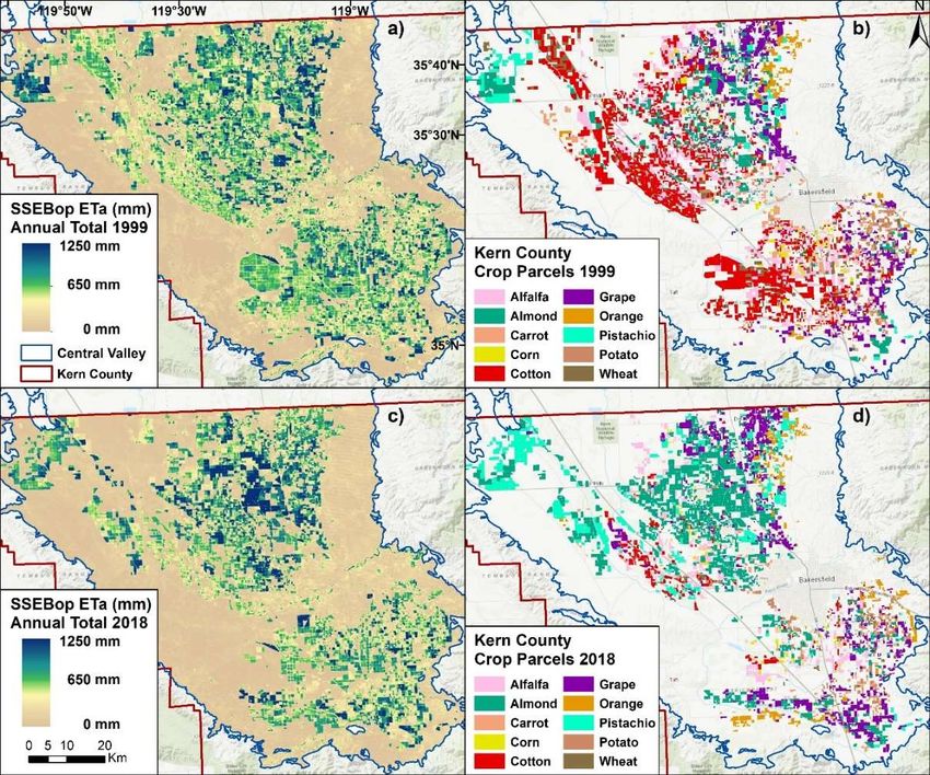
Remote Sens. 2019, 11, 1782                                                                          2 of 22

hydrologic sub-basins in the middle and lower Central Valley and demonstrated the reliability in
estimating water use over time with remote sensing. In this study, Landsat imagery was processed
through the Operational Simplified Surface Energy Balance (SSEBop) model which integrates weather
and remotely sensed images to estimate monthly and annual ETa [6]. This study is the first of its kind
to model 30-m resolution actual evapotranspiration from thermal remote sensing for the entire Central
Valley to estimate crop water use in irrigated agriculture for the period 2008–2018.
     Irrigated agriculture relies on both groundwater and surface water fed by annual precipitation [7].
On average, 80% of surface water in the Central Valley comes primarily from snowmelt off the
Sierra Nevada Mountains, which provide the primary water source for rivers and streams that feed
the hydrologic system across the state [3]. However, in 2015 alone, persistent drought conditions
substantially strained agricultural production with an estimated economic cost of $2.7 billion [1].
During droughts, growers in the Central Valley make up for surface water shortages through expanded
use of aquifers [8]. Groundwater plays a critical role in the agricultural sector as it supplies up to
50% of irrigation water in drought years [1]. In 2014, the California Department of Water Resources
determined that groundwater levels in 55% of long-term wells in the San Joaquin Valley and 36% of
the long-term wells in the Sacramento Valley had declined to levels approaching or surpassing historic
lows [7].
     During the last 11 years, there have been two major drought events in the Central Valley—the
2007–2009 drought and the most recent 2012–2016 drought. Thomas, et al. [9] noted that the Palmer
Drought Stress Index (PDSI) identified June–July 2014 as the most severe drought index in the Central
Valley going back to the beginning of the 20th Century. Several studies have noted the 2012–2016
drought as potentially the most severe in the last 1000 years based on the soil moisture index [8,9].
Famiglietti, et al. [10] estimated total consumptive use of groundwater in the valley and determined
that groundwater resources in the Central Valley were being depleted since 2000. Xiao, et al. [8] found
that the rates of groundwater storage decline were higher during the last two drought events, and
although they recovered somewhat during non-drought years, the 2012–2016 drought showed the
highest rate of decline in comparison to the long-term average. This research indicates the extent to
which growers relied on groundwater resources during periods of substantial drought.
     Other researchers have used remote sensing-derived ETa to study crop water use in the Central
Valley. Szilagyi and Jozsa [11] found that irrigation ETa has generally declined after the turn of the
century and that the ETa to precipitation ratio has gradually increased. Semmens, et al. [12] modeled
daily ETa for the 2013 growing season in two grape vineyards on the border between Sacramento and
San Joaquin Counties. Shivers, et al. [13] demonstrated with hyperspectral imagery that total crop area
had decreased as drought persisted in 2013–2015 and found that alfalfa and cotton declined in area
from 2013 to 2015 whereas almonds and pistachios showed overall greater resilience.
     Anderson, et al. [14] constructed an ET data cube for the 2015–2016 water year over the California
Delta region to provide field-scale water use estimates. They noted that water use analysis for California
frequently utilizes water balance or crop coefficient techniques to estimate crop ETa, which may bias
the results as they are idealized estimates that neglect real-world factors that limit crop ETa. They
argued that diagnostic ETa techniques provided by thermal remote sensing reflects actual conditions
and water management behaviors across landscapes [14]. Senay, et al. [5] took a similar approach
with thermal remote sensing to determine water use estimates and modeled SSEBop monthly and
annual ETa for 1984–2014 for selected hydrologic unit code (HUC)-8 sub-basins in the middle and
lower Central Valley.
     While several studies, including those listed here, have focused on site-specific analysis of remote
sensing-based ETa, this study is the first study to use a remote sensing approach and map actual
evapotranspiration for the entire Central Valley of California since 2008. With companion crop
classification data for the scale of the Central Valley, we investigated how different crops in the Central
Valley utilize water and how crop water use changes over time. We evaluated crop water use at
three scales of analysis: the scale of the entire Central Valley, at the county scale, and at the scale of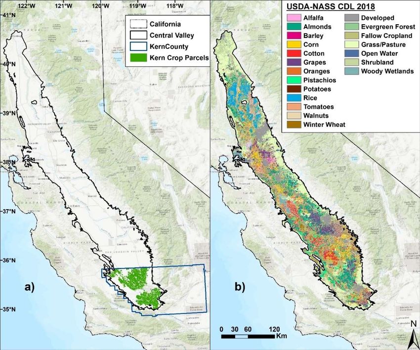
Remote Sens. 2019, 11, 1782 3 of 22
individual fields. At the scale of the entire Central Valley, the only crop classification dataset at the
same large spatial scale is the U.S. Department of Agriculture, National Agricultural Statistics Service
(USDA-NASS) Cropland Data Layer (CDL), which is available from 2008 to2018 and allows analysis of
large changes for the entire valley over the last decade. At the county level and field level, we utilized
crop parcel data from Kern County, which is available from 1999 to 2018, and expand the3time-series
Remote Sens. 2019, 11, x FOR PEER REVIEW of 22
to
20 years of change but at a smaller spatial scale. We also examined pixel-based trends and field-scale
water useofpatterns
large changes
in Kern for the entire from
County valley 1999
over the last decade.
to 2018 At the
to better county level
understand and field level,
small-scale we in crop
changes
utilized crop parcel data from Kern County, which is available from 1999 to 2018, and expand the
water use over time. This study demonstrates how a remote sensing-derived surface energy balance
time-series to 20 years of change but at a smaller spatial scale. We also examined pixel-based trends
model can be applied using crop classification data at multiple spatiotemporal scales to analyze trends
and field-scale water use patterns in Kern County from 1999 to 2018 to better understand small-scale
in historical water
changes use,water
in crop including
use overthe response
time. ofdemonstrates
This study crop water how
use atoremote
prolonged droughtsurface
sensing-derived conditions.
energy balance model can be applied using crop classification data at multiple spatiotemporal scales
to analyze
2. Materials trends in historical water use, including the response of crop water use to prolonged
and Methods
drought conditions.
2.1. Study Area
2. Materials and Methods
The Central Valley, as shown in Figure 1a, is a large flat valley that covers over 52,000 km2 and
dominates2.1.the
Study Area portion of California extending nearly 720 km along a northwest–southeast
central
axis [15,16]. The
TheCentral
Central Valley, as shown
Valley in Figure of
is composed 1a, the
is a large flat valleyValley
Sacramento that covers overnorth,
in the 52,000 the
km 2 San
and Joaquin
Valley indominates
the center,theand
central
the portion
semi-aridof California extending
Tulare Basin at thenearly 720 km along
southernmost enda northwest–southeast
[16]. The Central Valley is
borderedaxis
by [15,16]. The Central
the Shasta NationalValley is composed
Forest of the Sacramento
on the north, the coastalValley
rangein including
the north, the San Joaquin
major coastal cities to
Valley in the center, and the semi-arid Tulare Basin at the southernmost end [16]. The Central Valley
the west,isthe Sierra Nevada Mountains to the east (which provide much of the surface water), and
bordered by the Shasta National Forest on the north, the coastal range including major coastal cities
the Mojave Desert to the
to the west, the southeast.
Sierra The Central
Nevada Mountains to the Valley hasprovide
east (which a Mediterranean climate
much of the surface especially
water), and in the
southernthe Mojave Desert to the southeast. The Central Valley has a Mediterranean climate especially in the
part with hot, dry summers and mild, wet winters with most of the precipitation falling
between southern
November part and
with March
hot, dry[17].
summersKernand mild, wet
County winters with
comprises the most of the precipitation
southernmost sectionfalling
of the Central
between November and March [17]. Kern County comprises the southernmost section of the Central
Valley and includes the city of Bakersfield. The county is bordered by the Greenhorn Mountains to
Valley and includes the city of Bakersfield. The county is bordered by the Greenhorn Mountains to
the northeast, the Antelope Valley to the southeast, and the Temblor Range in the west. Agricultural
the northeast, the Antelope Valley to the southeast, and the Temblor Range in the west. Agricultural
commodities in Kern
commodities in County
Kern Countywere valued
were valuedatatover
over $7.25 billion
$7.25 billion in in 2017
2017 [18].[18].
Figure 1.Figure 1. The Central
The Central ValleyValley of Californiashowing
of California showing (a)
(a)the
thevalley
valleyboundary used in
boundary this in
used study
thisalong
study along
with Kernwith Kern and
County County
the and
KerntheCounty
Kern County Crop Parcels;
Crop Parcels; and (b)andthe(b)2018
the U.S.
2018 Department
U.S. Department of
of Agriculture,
National Agricultural Statistics Service (USDA-NASS) Cropland Data Layer for the Central Valley.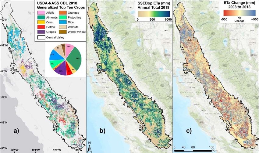
Remote Sens. 2019, 11, 1782                                                                        4 of 22

     We estimated crop water use for these areas by combining SSEBop ETa annual estimates with
crop classifications. The crop classification grid is at the same 30-m resolution and is created by the
USDA-NASS which provides annual grids from 2008 to 2018 [19]. The most recent USDA-NASS CDL
for 2018 is shown in Figure 1b.

2.2. Landsat
     This study utilized Google Earth Engine (GEE) cloud-based processing and the SSEBop approach
on Landsat remote-sensing imagery to calculate annual actual evapotranspiration at 30-m resolution.
GEE was used to generate annual ETa estimates for the entire Central Valley for the years 2008–2018, as
well as for the last 20 years (1999–2018) for Kern County. For the annual Central Valley ETa, all Landsat
Collection 1 Top-of-Atmosphere imagery from 13 Path/Rows (Path 41 Rows 35–36, Paths 42 Rows
34–36, Paths 43 Rows 33–35, Paths 44 Rows 32–34, and Path 45 Rows 32–33) was collected, totaling
4843 Landsat scenes, and processed. This imagery includes 839 Landsat 5 scenes (17%), 2602 Landsat
7 scenes (54%), and 1402 Landsat 8 scenes (29%) with an average of 430 images for each year or 33
images for each Path/Row. This number exceeds the suggested minimum of 10–12 images per year for
each Path/Row recommended to generate a reliable remote sensing-derived ETa estimate [20].
     Due to the heavy computer resource and processing requirements for ingesting millions of Landsat
pixels for the entire Central Valley for multiple years, the SSEBop model has been implemented in the
Google Earth Engine processing environment, which provides large-scale processing of thousands
of Landsat images [21]. Processing that would normally take weeks or months can now be done in
a matter of days. All Landsat pixels containing the Central Valley were processed in GEE using the
SSEBop model as well as new cloud-based interpolation and aggregation algorithms for all scenes with
60% cloud cover or less. This includes masking clouds using the Landsat Quality Assessment band and
Landsat 7 scan-line errors and filling these pixels through linear interpolation from contemporaneous
scenes (within 48 days before/after an image) [22].

2.3. The SSEBop Modeling Approach
     The Operational Simplified Surface Energy Balance (SSEBop) model is a thermal remote sensing
method that ingests Landsat imagery and generates daily total actual evapotranspiration (ETa) [6]. The
primary product of the method is the ET fraction, driven by land surface temperature (Ts) from the
Landsat thermal band, which takes a fractional amount of alfalfa-reference potential ET (ETr) derived
from GridMET to create actual ET [5,6,23]. GridMET is a gridded dataset at 4-km resolution provided
by the University of Idaho that provides daily weather variables for the continental United States from
1979 to present [23]. SSEBop ETa is driven by the thermal band from Landsat 5/7/8 satellites, which is
processed at the native spatial resolution—Landsat 5 (120 m), Landsat 7 (60 m), Landsat 8 (100 m)—but
then resampled to 30 m. This method is described in detail in Senay [6]. SSEBop actual ET can be
summarized with the following equation:

                                     ETa = (1 − γs (Ts − Tc )) ∗ ETr                                  (1)

where ETa is actual ET (mm); ETr is alfalfa-reference (maximum potential) ET (mm) from GridMET
which represents the maximum amount of daily water use under optimal water supply conditions; Ts is
the land surface temperature derived from the Landsat thermal band (K); Tc is the cold/wet limit, derived
from gridded maximum air temperature (K) representing the surface temperature at which maximum
evapotranspiration is occurring; and γs is a surface psychrometric constant (K) [6]. The GridMET ETr
has been bias-corrected with a coefficient of 0.85 derived from a comparison with California Irrigation
Management Information System (CIMIS) station data (https://cimis.water.ca.gov/).
      Similar to Senay, et al. [22], before ETa was computed for each scene, cloud-masked pixels were
filled using per-pixel linear interpolation from images 48 days before and after the scene date. Daily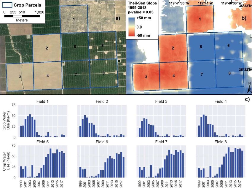
Remote Sens. 2019, 11, 1782                                                                         5 of 22

ETa was calculated using Equation (1) in GEE along with daily GridMET ETr and then aggregated to
the annual total.
     The relative accuracy of SSEBop ETa has been evaluated multiple times and shown to match
well with Ameriflux eddy-covariance flux towers as well as Max Planck Institute monthly ETa,
demonstrating that SSEBop can detect spatial variability and monthly and annual trends with
reasonable accuracy [20,22,24–27]. In Senay, et al. [5], we compared monthly SSEBop ETa to monthly
MPI ETa from 1984 to 2011 for eight HUC-8 sub-basins in the middle and lower Central Valley and
found an average r2 of 0.76 and average root mean square error (RMSE) of 11.7 mm. More recently, we
compared monthly SSEBop ETa to Ameriflux eddy-covariance flux tower monthly ETa in the Upper
Rio Grande Basin for non-cropland environments such as forest, shrubland, and grassland sites from
2007 to 2014 and found an average r2 of 0.85 and average normalized RMSE of less than 10% [22].

2.4. USDA-NASS Cropland Data Layer (CDL)
      The USDA-NASS provides cropland data layers (CDL) for the United States from 2008 to present,
which includes spatially explicit land use and land cover classification at 30-m resolution [19]. The CDL
is released each year and is meant to represent crop-specific land cover—classifications for over 100
individual crop types—from the previous year’s growing season [28]. The CDL is primarily derived
from Landsat 5, 7, and 8 imagery as well as other remote sensing datasets such as Deimos-1 imagery
and the National Land Cover Database (NLCD) in a decision-tree classification algorithm [28,29]. The
CDL originally provided 30-m resolution data from 2010, whereas 2008/2009 data were provided in
coarser resolution; however, recently, USDA-NASS reprocessed 2008/2009 CDL to match the spatial
resolution of the other CDL datasets from 2010 onwards [19]. The accuracy reported by USDA-NASS
for the large-area crops ranges from 85 to 95% [29].
      The CDL is the best crop-specific gridded dataset available for the entire Central Valley
Lark, et al. [28], in a review of the use of USDA-NASS CDL in scientific publications, noted several
potential biases and recommendations, which we included in this study as detailed in Section 2.5. For
this study, only the 10 most expansive crops (in total area) between 2008 and 2018 for the Central
Valley were utilized to summarize ETa. These 10 crops (alfalfa, almonds, corn, cotton, grapes, oranges,
pistachios, rice, walnuts, and winter wheat) were selected from the larger dataset and other CDL
classes were discarded. The top 10 crops in the Central Valley comprise about 17,000 km2 or roughly
33% of the valley area. Misidentified pixels are widely dispersed and isolated in marginal areas, so
they were removed for the major CDL crops through a generalization procedure to retain only pixel
clusters of 8 or more neighboring pixels. This resulted in a cleaner classification grid that more closely
aligns with visual crop fields with minimal reduction in total crop area.

2.5. County Crop Acreage Reports
     To estimate the area for the major crops in the entire Central Valley using the generalized CDL,
we estimated area using the pixel-counting method but then bias-corrected based on a comparison
with the county-reported annual crop reports provided by each individual county’s Agricultural
Commissioner. The reported area from each California county was collected from the local Agricultural
Commissioner’s annual reports for each major crop similar to the method used in Fulton, et al. [30];
annual county crop reports are publicly available through the California Department of Food and
Agriculture (https://www.cdfa.ca.gov/exec/county/CountyCropReports.html).
     The county crop areas were then aggregated up to the scale of the entire Central Valley and
compared to the area estimates from the annual generalized USDA-NASS CDL. On average, the
generalized CDL overestimated crop area by 4% or 6100 ha for all 10 crops. The average bias was
determined at the scale of the entire Central Valley for each major crop by comparing the generalized
CDL area against the aggregated county reported numbers from 2008 to 2017 (the 2018 acreage reports
were not yet available at the time of this writing) and is included in Table 1. Crops such as almonds,
cotton, rice, and walnuts were all estimated by the CDL to within 5% of the county crop reports.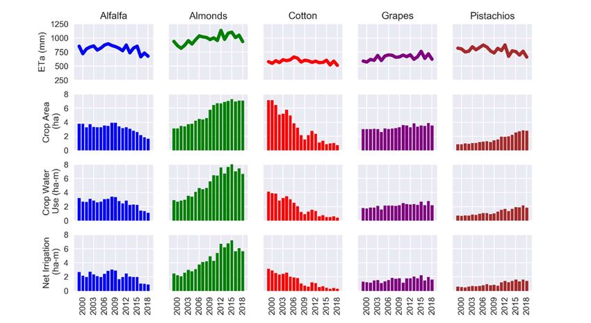
Remote Sens. 2019, 11, 1782                                                                                  6 of 22

      Table 1. Comparison of the area counts between the USDA-NASS Generalized Cropland Data Layer
      (CDL) and the aggregated county crop acreage reports from 2008 to 2017 for the top 10 crops in the
      Central Valley showing: (1) the average crop area in hectares from pixel-counting the generalized CDL,
      (2) the average crop area from the aggregated crop reports, and (3) the bias percentage that was used to
      bias-correct the CDL area to calculate water use between 2008 and 2018.

                          Crop Type               CDL 1            Crop Reports 1      % Bias
                           Alfalfa               285,164                247,669         15%
                         Almonds                 415,498                392,967         6%
                            Corn                  83,820                 62,504         34%
                           Cotton                111,169                108,328         3%
                          Grapes                 216,628                244,110        −11%
                          Oranges                 57,601                 65,721        −12%
                         Pistachios               75,978                 90,929        −16%
                            Rice                 215,794                208,871          3%
                          Walnuts                121,829                126,944        −4%
                        Winter Wheat             155,343                129,594        20%
                                       1   In hectares (ha). 1 hectare = 2.47 acres.

     The generalized CDL area for the entire Central Valley, including for 2018, for each major crop
was then bias corrected using the 2008–2017 average bias of each crop type displayed in Table 1. This
resulted in area estimates that were closer to the aggregated county-reported area in both magnitude
(within +/− 1%) and annual variation (average ’r’ correlation value of 0.79) for all major crops, especially
in alfalfa, almonds, cotton, rice, and walnuts. Overall, the bias correction of the generalized CDL
acreage estimates provided a much more accurate reading based on county acreage reports. Estimating
the area accurately was crucial in determining the volume of water use for each crop as part of this
study; the water use estimates are dependent on not just the accuracy of the ET model but also heavily
impacted by the area count utilized.

2.6. Kern County Crop Boundaries
     The Kern County Department of Agriculture and Measurement Standards provides digitized
annual crop parcel boundaries for all of Kern County from 1997 to the present (http://www.kernag.
com/gis/gis-data.asp) as used in Shivers, et al. [13]. The crop parcel boundaries provide county-scale
crop type classification for Kern County with a wider temporal extent (1999–2018) as well as more
accurate area estimates than the estimated CDL area, and cleaner crop sampling zones for ETa sampling.
For the analysis of Kern County crop water use from 1999 to 2018, the area counts reported in each
parcel boundary were collected, aggregated, and used to create volumetric water use from SSEBop
ETa without any bias correction on the area, as was done with the USDA-NASS CDL, but instead
were assumed to be accurate counts. The crop parcel boundaries were an invaluable dataset to this
study as an expansion on the crop data information provided by USDA-NASS. Not only does this
dataset provide a longer time-series of crop type information dating back to 1999, it also provides more
accurate area estimates for each parcel. When compared to the generalized CDL area counts for the
matching crops in Kern County, the CDL accurately identifies 87% of the crop parcels produced by
Kern County—underestimating the crop area by 13%.
     Many of the parcels that the CDL failed to identify had low Normalized Difference Vegetation
Index (NDVI) values suggesting that these parcels may not have been actively farmed in that year.
Because we considered only “active crop parcels”, the Kern County crop parcels were filtered in each
year for parcels that averaged ≥ 0.5 in May–September maximum NDVI, and so, only these parcels
were included for further analysis. Water use was determined using the area provided with the crop
parcel dataset for those parcels that were “active”. To maintain consistency with the CDL summaries
for the entire Central Valley, the SSEBop ETa was averaged for each crop type and converted into
volumetric water use estimate for each year using the corresponding crop area.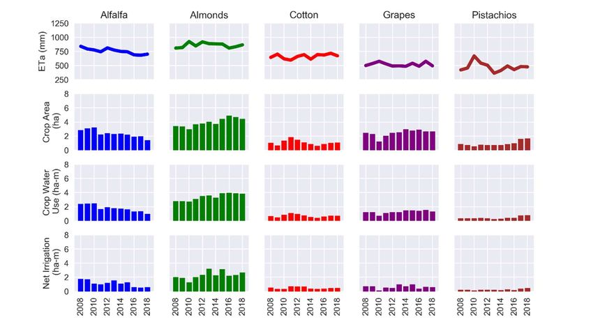
Remote Sens. 2019, 11, 1782                                                                        7 of 22

2.7. Other Datasets
     Other remote sensing datasets utilized included gridded annual total precipitation for the Central
Valley for the 1999–2018 period extracted from 4-km PRISM (Parameter-elevation Regressions on
Independent Slopes Model) precipitation datasets in order to calculate net irrigation [31].
     Additionally, maximum NDVI was derived from Landsat to determine the “active” crop parcels
in Kern County crop boundaries described in the previous section. The May–September maximum
Landsat surface reflectance NDVI was created in GEE for the period of 1999–2018. The May–September
seasonal maximum was chosen to identify crop boundaries that were actively vegetated in the peak
growing season while not being rainfed. According to PRISM, the May–September period has the
lowest precipitation totals for the valley in the 1999–2018 period annually ranging from 3–55 mm and
averaging 18 mm as opposed to the April–October period which annually ranges from 90–500 mm and
averages 315 mm.
     The shapefile of the Central Valley was acquired from the U.S. Geological Survey’s Central
Valley Hydrologic Model, which provides the digital extent of the alluvial deposits of the contiguous
Sacramento, San Joaquin, and Tulare Lake groundwater basins and encompasses an approximate
50,000 km2 area of central California [16].

2.8. Water Use Estimates and Net Irrigation
    To calculate crop water use in volumetric units, the spatially-averaged SSEBop annual ETa (mm)
was determined for each crop type at each scale of analysis and then converted into hectare-meters
(ha-m) using the corresponding crop area as follows:

                                   Crop Water Use = ETa ∗ Crop Area                                   (2)

where Crop Water Use (ha-m) is the volume of water used by a specific crop in a given year, ETa (m) is
the spatially averaged SSEBop ETa for a given crop, and Crop Area (ha) is the surface area of the crop.
     One ha-m is equal to 10,000 m3 (8.11 ac-ft). For net irrigation, the annual precipitation is
subtracted from the annual ETa. It is important to note that assuming all precipitation is effective may
underestimate the net irrigation amount.

2.9. Trend Analysis
      For the time-series analysis of crop ETa, the simple Mann–Kendall (MK) trend test was used
to test the presence or absence of statistically significant trends in water use at both the county and
valley scale as well as the scale of individual pixels. The MK test is a non-parametric rank-based
method for identifying monotonic trends and is widely used in time-series analysis of hydrologic
data [32–35]. This test examines the slopes between pairwise samples ranked chronologically and
results in an overall MK score that indicates a positive or negative trend along with 95% confidence
level (p-value < 0.05) [33,35]. We tested for serial correlation in the sample with the Durbin–Watson
statistic (not shown) prior to running the MK test and we found that there was no serial correlation in
the statistically significant results. The Theil–Sen estimator was then used to measure the magnitude
of the slope over the study period. The Theil–Sen estimator is a non-parametric alternative to the
parametric ordinary least squares regression line and is frequently used alongside the Mann–Kendall
test in hydrologic time-series analysis [35,36].
      One limitation of the MK test is that it requires a minimum of 8–10 data samples to provide a
statistically significant result. There are 11 years’ worth of USDA-NASS CDL (2008–2018) and therefore
a maximum of 11 annual crop ETa data points which meets the minimum requirement of the test;
however, low sample size may affect the ability to detect statistically significant trends in some crops.
The MK test was utilized to detect trends in SSEBop ET summarized by USDA-NASS CDL as well
as water use characterized by the Kern County crop boundaries from 1999 to 2018. Additionally, the
MK test was conducted on a per-pixel basis for all SSEBop annual ETa in Kern County for 1999–2018.
Remote Sens. 2019, 11, x FOR PEER REVIEW 8 of 22
Remote Sens. 2019, 11, 1782 8 of 22
CDL as well as water use characterized by the Kern County crop boundaries from 1999 to 2018.
Additionally, the MK test was conducted on a per-pixel basis for all SSEBop annual ETa in Kern
The per-pixel MK uses the same statistical process and produces the same resulting MK statistic,
County for 1999–2018. The per-pixel MK uses the same statistical process and produces the same
Theil–Sen
resultingslope, and p-value,
MK statistic, but slope,
Theil–Sen conducts
and the test for
p-value, buteach pixelthe
conducts in test
the for
time-series
each pixelstack oftime-
in the annual
grids. The
series results
stack of this grids.
of annual 20-year “trend
The grid”
results were
of this then “trend
20-year contextualized
grid” werein the
thendiscussion on individual
contextualized in the
discussion on individual fields within Kern County and how the shifting crop types of those
fields within Kern County and how the shifting crop types of those fields affected trends fieldsuse
in water
overaffected trends in water use over time.
time.
3. Results
3. Results
3.1.3.1.
Crop Water
Crop Use
Water ininthe
Use theCentral
CentralValley
Valley2008–2018
2008–2018
TheThe
toptop
1010 majorcrops
major cropsforforthe
theentire
entire Central
Central Valley,
Valley, in
inarea,
area,are
arealfalfa,
alfalfa,almonds,
almonds, corn, cotton,
corn, cotton,
grapes, oranges, pistachios, rice, walnuts, and winter wheat. Figure 2a displays the geographic spread
grapes, oranges, pistachios, rice, walnuts, and winter wheat. Figure 2a displays the geographic spread
andand relative
relative distributionofofthese
distribution these1010crops
cropsfor
for the
the year
year 2018,
2018,the
themost
mostrecent
recentyear
year that
thatthethe
CDLCDLdata is is
data
available
available at at
thethe time
time ofofwriting.
writing.Although
Although thethe total
total area
areaofofthese
thesetop
top1010crops
cropsstays
staysrelatively
relativelystable
stable
over
over thethe 2008–2018
2008–2018 periodatatabout
period about1.6
1.6million
million ha,
ha, the
the distribution
distributionofofthe
thecrops
cropsshifts over
shifts overtime. While
time. While
crops such as cotton or rice stayed relatively stable over this period, other crops such
crops such as cotton or rice stayed relatively stable over this period, other crops such as alfalfa and as alfalfa and
winter
winter wheat
wheat declinedininarea
declined areawhile
whilenutnut crops
crops such
such as
as almonds,
almonds,pistachios,
pistachios, andandwalnuts
walnuts increased.
increased.
These shifts in preferred crops greatly influenced the water use patterns in the
These shifts in preferred crops greatly influenced the water use patterns in the Central Valley. Central Valley.
Figure 2. The Central Valley for 2018 showing (a) the generalized top 10 crops identified by USDA-NASS
Figure 2. The Central Valley for 2018 showing (a) the generalized top 10 crops identified by USDA-
CDL, (b) the SSEBop annual total actual ET for 2018, and (c) the change in SSEBop ETa from 2008 to
NASS CDL, (b) the SSEBop annual total actual ET for 2018, and (c) the change in SSEBop ETa from
2018 (2018
2008 ETa (2018
to 2018 minusETa
2008 ETa).2008 ETa).
minus
SSEBop
SSEBop ETa, such
ETa, suchasasthe
the2018
2018annual
annualtotal
total shown
shown in in Figure
Figure2b, 2b,can
canshow
showa bird’s
a bird’s
eyeeye view
view of the
of the
spatial variability
spatial variability and
andrelative
relativewater
wateruse
use across the entire
across the entirevalley,
valley,andandcrop
croptype
type information
information provides
provides
valuable context to understand these patterns. For instance, the rice fields identified
valuable context to understand these patterns. For instance, the rice fields identified in the CDL, in the CDL, which
arewhich are frequently flood-irrigated, are detected in the 2018 SSEBop ETa as dark blue signifying or
frequently flood-irrigated, are detected in the 2018 SSEBop ETa as dark blue signifying 1000 mm
1000
more ofmm
ETa or
in more of ETa
a given year. in The
a given
ETayear.
changeThemap
ETa change
in Figuremap 2cinshows
Figurebright
2c shows
bluebright bluesame
in these in these
fields
same fields
indicating indicating
a positive a positive
change of upchange
to 500 ofmmup in
to 2018
500 mm in 2018 astoopposed
as opposed 2008, but to 2008, but aslater
as shown shown
in the
later in the Mann–Kendall
Mann–Kendall trend results, trend results,
the trend the overall
in rice trend indecreases.
rice overallThese
decreases. These ETa
ETa change maps change mapsbut
are useful
are useful
sampling andbut sampling
charting and charting
the entire the entire
time-series time-series
provides provides
more detail thanmore detailotherwise
we would than we would
see.
otherwise see.
Table 2 presents the averages for the final bias-corrected crop area estimates as well as the difference
between the last year (2018) and the first year (2008) for the top 10 major crops. The area estimates
demonstrate a substantial decline in alfalfa and winter wheat and substantial increases in nut cropsRemote Sens. 2019, 11, 1782 9 of 22
such as almonds, pistachios, and walnuts from the first year of the study in 2008 to the last year in 2018.
Almonds are distributed throughout the valley and do not seem to decrease during the 2012–2016
drought. In fact, almonds show an increase of 30% in 2018 as compared to 2008. Other crops that see
an increase in area are grapes, pistachios, and walnuts while alfalfa, corn, oranges, and winter wheat
all see decreases in 2018 as opposed to 2008, which changes their overall water use totals.
Table 2. Summary statistics of the final bias-corrected area estimates for the top 10 major crops in
the Central Valley from 2008 to 2018 ordered by mean area including: (1) the 2008–2018 mean crop
area in hectares, (2) the crop area in 2008 including the percentage of the total, (3) the crop area in
2018 including the percentage of the total, (4) the % change in crop area between 2008 and 2018, and
(5) the mean crop area during the 2012–2016 California drought including the percent deviation from
the mean.
Mean Crop 2008 Crop Area 2018 Crop Area 2012–2016 Drought
Crop Type % Change
Area (ha) 1 (ha) 1 [%] (ha) 1 [%] (ha) 1 [%]
Almonds 395,204 343,695 [21%] 445,249 [27%] 30% 417,652 [6%]
Grapes 246,339 243,992 [15%] 268,246 [16%] 10% 273,978 [11%]
Alfalfa 235,705 283,905 [18%] 141,768 [9%] −50% 223,405 [−5%]
Rice 208,336 210,712 [13%] 200,805 [12%] −5% 203,405 [−2%]
Walnuts 130,527 92,920 [6%] 161,005 [10%] 73% 129,912 [< −1%]
Winter Wheat 118,101 146,169 [9%] 62,256 [4%] −57% 108,738 [−8%]
Cotton 109,195 104,663 [6%] 107,219 [7%] 2% 99,718 [−9%]
Pistachios 93,545 87,790 [5%] 167,678 [10%] 91% 81,230 [−13%]
Corn 62,738 69,604 [4%] 59,031 [4%] −15% 59,411 [−5%]
Oranges 27,152 26,837 [2%] 18,619 [1%] −31% 26,810 [−1%]
1 In hectares (ha). 1 hectare = 2.47 acres.
Trend analysis, using the MK test, reveals the crops that show statistically significant increases
or decreases in crop area and the results are displayed in Table 3 for the 10 major crops. The results
highlight that almonds, grapes, pistachios and walnuts all have statistically significant increasing trends
over the 2008–2018 period whereas alfalfa and winter wheat have statistically significant decreasing
trends. This analysis confirms that almonds and other fruit and nut crops are increasing in crop area
over time in the Central Valley while more traditional row crops such as alfalfa are seeing declines in
crop area over the same period. The remaining crops did not show a significant trend although it can
be inferred from the slope that corn, cotton, and rice decreased in area over the 11-year period.
Table 3. Simple Mann–Kendall trend test results for CDL crop area in the Central Valley from 2008 to
2018 for the top 10 major crops showing: (1) Mann–Kendall trend statistic, (2) p-value, (3) Theil–Sen
slope (ha/year) from 2008 to 2018, and (4) the significant trend where (+) and (−) indicate statistically
significant increasing or decreasing trends, respectively, where the p-value is less than 0.05 and
(#) signifies the trend is not statistically significant and the p-value is greater than 0.05.
Crop Type MK Statistic p-Value Theil–Sen Slope (ha/yr) 1 Trend 2
Alfalfa −39 0.003 −12,429 −
Almonds 39 0.003 16,327 +
Corn −21 0.119 −3543 #
Cotton −9 0.533 −2038 #
Grapes 29 0.029 6119 +
Oranges −1 1.000 −48 #
Pistachios 27 0.043 6635 +
Rice −23 0.087 −3411 #
Walnuts 49 0.000 6668 +
Winter Wheat −37 0.005 −7770 −
1 In hectares (ha). 1 hectare = 2.47 acres, 2 Durbin–Watson statistic shows no serial correlation for the statistically
significant trends.Remote Sens. 2019, 11, 1782 10 of 22
Remote Sens. 2019, 11, x FOR PEER REVIEW 10 of 22
These shifting patterns in crop area impact the overall water use for the major crop types. Figure 3
shows theThese shifting
ETa, crop areapatterns in crop
(ha), water usearea impact
(ha-m), andthenetoverall water
irrigation use for
(ha-m) theremoving
after major crop alltypes. Figure
precipitation
3 shows
for five of the the
top ETa, cropinarea
10 crops (ha), water
the valley. use (ha-m),
The annual and of
variation netETa
irrigation
is small (ha-m) after removing
in comparison all
to crop area
precipitation for five of the top 10 crops in the valley. The annual variation of ETa is small in
which has a large impact on overall water use. The total annual crop water use for the top 10 crops
comparison to crop area which has a large impact on overall water use. The total annual crop water
in the Central Valley averages over 1.19 million ha-m. The primary water users in 2008 are alfalfa,
use for the top 10 crops in the Central Valley averages over 1.19 million ha-m. The primary water
almonds, and rice, which each consume around 20% of the total crop water use for the valley’s major
users in 2008 are alfalfa, almonds, and rice, which each consume around 20% of the total crop water
crops. By 2018, that share of crop water use shifts and alfalfa is only 9% of the total water use while
use for the valley’s major crops. By 2018, that share of crop water use shifts and alfalfa is only 9% of
almonds increase
the total water to use
33%while
(see Table 4). Rice
almonds and winter
increase to 33%wheat see more
(see Table modest
4). Rice and declines in their
winter wheat seeshare
moreof
watermodest
use while
declines in their share of water use while pistachios and walnuts see modest increases. or
pistachios and walnuts see modest increases. The remaining crops show minimal Theno
real change in the proportion of total water use shifting +/−
remaining crops show minimal or no real change in the proportion of total water use shifting +/− 4%
4% of the total from 2008 to 2018. However,
of the totalinfrom
the difference each2008 to 2018.
crop’s waterHowever,
use fromthe thedifference
first year inof each crop’sin
the study water
2008useandfrom the first
the last yearyear of
in 2018
the study
displays somein 2008 andshifts
dramatic the last year in 2018
as indicated displays
in Table some dramatic
4. Alfalfa, shifts asrice,
corn, oranges, indicated in Table
and winter 4.
wheat
Alfalfa, corn, oranges, rice, and winter wheat all declined in 2018 as compared to 2008 whereas
all declined in 2018 as compared to 2008 whereas almonds, pistachios, and walnuts saw dramatic
almonds,
increases. pistachios,
Cotton and walnuts
and grapes also saw saw dramatic
increases increases.
but much more Cotton and grapes
modest. also saw
Pistachios increases
showed but
the most
muchchange
dramatic more modest.
with a Pistachios
115% increase showed the most
in 2018 dramatic to
as compared change
2008 with a 115%
although theincrease in 2018
total share as
of crop
compared to 2008 although the total share of crop water use was still less
water use was still less than 10%. Alfalfa saw the most dramatic decline both in the percentage drop than 10%. Alfalfa saw the
mostindramatic
but also magnitude decline
and both in theofpercentage
the share total crop drop
waterbut also
use. Inin magnitude
2008, and the
alfalfa used shareha-m
238,316 of total
of crop
water
but 11 years later, the crop used less than 100,000 ha-m, a 58% decline. Table 4 also displays the than
water use. In 2008, alfalfa used 238,316 ha-m of water but 11 years later, the crop used less mean
100,000 ha-m, a 58% decline. Table 4 also displays the mean crop water use for the 2012–2016
crop water use for the 2012–2016 California drought as well as the percent decline from the 2008–2018
California drought as well as the percent decline from the 2008–2018 mean. Almost all 10 crops saw
mean. Almost all 10 crops saw a decline in mean water use during the drought, with the exceptions
a decline in mean water use during the drought, with the exceptions of almonds (7% above the mean)
of almonds (7% above the mean) and grapes (8% above the mean). Even under regional drought
and grapes (8% above the mean). Even under regional drought conditions, almonds still averaged
conditions, almonds still averaged 364,074 ha-m of water use per year. These results demonstrate that
364,074 ha-m of water use per year. These results demonstrate that almonds continue to be productive
almonds
in thecontinue to be productive
Central Valley even in droughtin theconditions.
Central Valley even in drought conditions.
Figure 3. Top five crops in the Central Valley from 2008 to 2018 showing the SSEBop ETa mean (in mm)
Figure 3. Top five crops in the Central Valley from 2008 to 2018 showing the SSEBop ETa mean (in
for the USDA-NASS CDL crop type, the bias-corrected area estimate (ha), water use volume (ha-m)
mm) for the USDA-NASS CDL crop type, the bias-corrected area estimate (ha), water use volume (ha-
and the net irrigation (ha-m). The area, water use, and net irrigation are scaled by 100,000 (i.e., 4 ha-m
m) and the net irrigation (ha-m). The area, water use, and net irrigation are scaled by 100,000 (i.e., 4
corresponds to 400,000 ha-m). 1 hectare = 2.47 acres. 1 hectare-meter = 8.107 acre-feet.
ha-m corresponds to 400,000 ha-m). 1 hectare = 2.47 acres. 1 hectare-meter = 8.107 acre-feet.
Table 4. Volumetric water use estimates for the top 10 major crops in the Central Valley from 2008 to
2018 ordered by the mean including: (1) the 2008–2018 mean water use, (2) the water use in 2008
including the percentage of the total, (3) the water use in 2018 including the percentage of the total,
(4) the % change in crop water use between 2008 and 2018, and (5) the mean crop water use during
the 2012–2016 California drought and percent deviation from the mean.Remote Sens. 2019, 11, 1782 11 of 22
Table 4. Volumetric water use estimates for the top 10 major crops in the Central Valley from 2008
to 2018 ordered by the mean including: (1) the 2008–2018 mean water use, (2) the water use in 2008
including the percentage of the total, (3) the water use in 2018 including the percentage of the total,
(4) the % change in crop water use between 2008 and 2018, and (5) the mean crop water use during the
2012–2016 California drought and percent deviation from the mean.
Mean Water 2008 Water Use 2018 Water Use 2012–2016 Drought
Crop Type % Change
Use (ha-m) 1 (ha-m) 1 [%] (ha-m) 1 [%] (ha-m) 1 [%]
Almonds 339,506 277,707 [23%] 385,230 [33%] 39% 364,074 [7%]
Rice 218,544 247,717 [21%] 197,711 [17%] −20% 213,144 [−2%]
Alfalfa 179,606 238,316 [20%] 99,308 [9%] −58% 168,856 [−6%]
Grapes 126,840 121,819 [10%] 132,561 [11%] 9% 136,772 [8%]
Walnuts 111,442 89,498 [7%] 130,072 [11%] 45% 110,900 [< −1%]
Cotton 71,508 67,374 [6%] 71,994 [6%] 7% 66,533 [−7%]
Winter Wheat 47,386 64,842 [5%] 18,601 [2%] −71% 40,980 [−14%]
Pistachios 44,123 37,028 [3%] 79,774 [7%] 115% 35,733 [−19%]
Corn 40,023 46,284 [4%] 34,039 [3%] −26% 38,042 [−5%]
Oranges 17,913 17,714 [1%] 10,940 [1%] −38% 16,825 [−6%]
1 In hectare-meters (ha-m). 1 hectare-meter = 8.107 acre-feet.
The MK trend analysis on crop water use, displayed in Table 5, corroborates the shifting trends in
Central Valley crop water use. Alfalfa and almonds have an inverse pattern to one another with alfalfa
showing a statistically significant declining trend in crop water use over the 2008–2018 period at a rate
of 13,901 ha-m per year. Conversely, almonds show a statistically significant increase in crop water
use at a rate of 13,488 ha-m per year. Other crops that have statistically significant increasing trends
are grapes and walnuts. On the other hand, crops such as rice and winter wheat show statistically
significant decreasing trends. Similar to the crop area, traditional row crops are declining in water use
over the 11-year period while fruit and nut crops are increasing in water use over the same period.
While the SSEBop ETa values taken independently provide a useful relative measure of water use in
the Central Valley, when contextualized and summarized by crop type, remote sensing can provide
easily interpretable and vital metrics for the consumption of water by major agricultural crops.
Table 5. Simple Mann–Kendall trend test results for CDL crop water use by volume in the Central Valley
from 2008 to 2018 for the top 10 major crops showing: (1) Mann–Kendall trend statistic, (2) p-value, (3)
Theil–Sen slope (ha-m/yr) from 2008 to 2018, and (4) the significant trend where (+) and (−) indicate
statistically significant increasing or decreasing trends, respectively, where the p-value is less than 0.05
and (#) signifies the trend is not statistically significant and the p-value is greater than 0.05.
Crop Type MK Statistic p-Value Theil–Sen Slope (ha-m/yr) 1 Trend 2
Alfalfa −41 0.002 −13,901 −
Almonds 35 0.008 13,488 +
Corn −23 0.087 −2756 #
Cotton −7 0.640 −841 #
Grapes 31 0.020 4042 +
Oranges −13 0.350 −382 #
Pistachios 25 0.062 1963 #
Rice −27 0.043 −5433 −
Walnuts 43 0.001 4300 +
Winter Wheat −35 0.008 −4086 −
1 In hectare-meters (ha-m). 1 hectare-meter = 8.107 acre-feet, 2 Durbin–Watson statistic shows no serial correlation
for the statistically significant trends.
3.2. County-Scale Crop Water Use—Kern County, 1999–2018
This same analysis was conducted on the scale of an individual county that has cropland in the
Central Valley to evaluate the county-scale change in crop water use. For the county-scale analysis, we
used the crop parcel shapefiles provided by Kern County from 1999 to 2018 to analyze 20 years of cropRemote Sens. 2019, 11, 1782 12 of 22
water use in Kern County rather than rely on the generalized USDA-NASS CDL, which is available
only from 2008 to present. Figure 4 displays the SSEBop ETa and crop classifications for Kern County
in the southernmost part of the Central Valley for the year 1999 and the year 2018. Total SSEBop ETa
does not show a clear increasing or decreasing trend in Kern County from 1999 to 2018 yet there are
Remote
clear Sens.
shifts in2019,
the11, x FOR PEER REVIEW
distribution of ETa across the county over time. 12 of 22
Figure
Figure 4. Kern
4. Kern County
County showing
showing (a)(a) 1999
1999 annual
annual total
total SSEBop
SSEBop ETa,
ETa, (b)(b) major
major commodity
commodity parcels
parcels in in
1999
1999 identified by Kern County Department of Agriculture and Measurement Standards and filtered by
identified by Kern County Department of Agriculture and Measurement Standards and filtered
by maximum
maximum NDVINDVI
≥ 0.5,≥ 0.5, (c) 2018
(c) 2018 annual
annual totalSSEBop
total SSEBopETa,ETa,and
and (d) major
majorcommodity
commodityparcels
parcelsin in
20182018
identified
identified byby Kern
Kern CountyDepartment
County Department of of Agriculture
Agriculture andandMeasurement
MeasurementStandards and
Standards filtered
and by by
filtered
maximum
maximum NDVI
NDVI ≥ ≥0.5.
0.5.
TheThetoptop
1010 crops
crops forKern
for KernCounty
Countyand and their
their crop
crop area
areaare
aredisplayed
displayedininTable
Table 6. 6.
TheTheactive
activecropcrop
parcels
parcels in in Kern
Kern Countyaverage
County averageover over205,000
205,000 haha from
from 1999
1999toto2018
2018but
butthere
thereis isa a
consistent
consistent decline
decline
overover
thethe 20-year
20-year periodatata arate
period rateofof1000
1000ha
ha per
per year.
year. Most
Mostofofthese
these“lost”
“lost”parcels
parcels seem
seem to to
occur
occursouth
south
of the city of Bakersfield where cotton and alfalfa fields predominated in the year
of the city of Bakersfield where cotton and alfalfa fields predominated in the year 1999, as shown 1999, as shown in in
Figure 4b. Overall, cotton seems to decline in favor of almonds from 1999 to 2018 in
Figure 4b. Overall, cotton seems to decline in favor of almonds from 1999 to 2018 in Figure 4. In 1999, Figure 4. In 1999,
cotton
cotton in Kern
in Kern County
County hadhad a production
a production valueofof$233
value $233million,
million,according
accordingtotocounty
county crop
crop reports,
reports, but
but by
2017, the production value of cotton fell to $74 million [18]. Almonds, on the other hand, increased
by 2017, the production value of cotton fell to $74 million [18]. Almonds, on the other hand, increased in
in value from $143 million in 1999 up to $1.26 billion by 2017 [18].
value from $143 million in 1999 up to $1.26 billion by 2017 [18].
Table 6. Summary statistics of the crop area estimates for the top 10 major crops in Kern County from
1999 to 2018 ordered by the mean including: (1) the mean of the 1999–2018 period, (2) the crop area
in 1999 and the percentage of the total crop area, (3) the crop area in 2018 and the percentage of the
total crop area, (4) the change in crop area between 1999 and 2018, and (5) the mean crop area during
the 2012–2016 California drought and percent deviation from the mean.
1999 Crop Area 2018 Crop Area
Crop Type Mean Crop Area (ha) 1 % Change 2012–2016 Drought (ha) 1 [%]
(ha) 1 [%] (ha) 1 [%]
Almonds 53,126 31,213 [14%] 70,924 [38%] 127% 69,662 [31%]
Cotton 32,957 71,264 [32%] 7,603 [4%] −89% 13,343 [−60%]
Grapes 32,778 30,261 [13%] 35,141 [19%] 16% 34,951 [7%]
Alfalfa 31,652 37,568 [17%] 16,438 [9%] −56% 27,922 [−12%]
Pistachios 16,247 8536 [4%] 27,908 [15%] 227% 22,693 [40%]
Oranges 11,305 7861 [3%] 11,484 [6%] 46% 12,565 [11%]
Wheat 9247 16,391 [7%] 2885 [2%] −82% 5566 [−40%]
Carrots 8952 10,964 [5%] 5537 [3%] −49% 8203 [−8%]Remote Sens. 2019, 11, 1782 13 of 22
Table 6. Summary statistics of the crop area estimates for the top 10 major crops in Kern County from
1999 to 2018 ordered by the mean including: (1) the mean of the 1999–2018 period, (2) the crop area in
1999 and the percentage of the total crop area, (3) the crop area in 2018 and the percentage of the total
crop area, (4) the change in crop area between 1999 and 2018, and (5) the mean crop area during the
2012–2016 California drought and percent deviation from the mean.
Mean Crop 1999 Crop Area 2018 Crop Area 2012–2016 Drought
Crop Type % Change
Area (ha) 1 (ha) 1 [%] (ha) 1 [%] (ha) 1 [%]
Almonds 53,126 31,213 [14%] 70,924 [38%] 127% 69,662 [31%]
Cotton 32,957 71,264 [32%] 7,603 [4%] −89% 13,343 [−60%]
Grapes 32,778 30,261 [13%] 35,141 [19%] 16% 34,951 [7%]
Alfalfa 31,652 37,568 [17%] 16,438 [9%] −56% 27,922 [−12%]
Pistachios 16,247 8536 [4%] 27,908 [15%] 227% 22,693 [40%]
Oranges 11,305 7861 [3%] 11,484 [6%] 46% 12,565 [11%]
Wheat 9247 16,391 [7%] 2885 [2%] −82% 5566 [−40%]
Carrots 8952 10,964 [5%] 5537 [3%] −49% 8203 [−8%]
Corn 5597 4633 [2%] 2622 [1%] −43% 5398 [−4%]
Potatoes 4913 7306 [3%] 6293 [3%] −14% 4216 [−14%]
1 In hectares (ha). 1 hectare = 2.47 acres.
Indeed, in the share of the total crop area for the top 10 crops, cotton occupies 32% of the active
crop parcels in 1999 but by 2018, cotton occupies 4% of the crop area. alfalfa shows a crop area decline
of 8%. Almonds, on the other hand, nearly triple in the share of total crop area up to 38% by 2018. The
change in crop area shows a consistent decline in traditional crops such as alfalfa, carrots, corn, cotton,
potatoes, and wheat while shifting towards investment in nut crops such as almonds and pistachios.
Even during severe drought conditions, such as 2012–2016, fruit and nut crops show an appreciable
increase in crop area, compared to the 20-year mean, whereas more traditional crops see substantial
declines, such as a 60% decrease in crop area for cotton and a 40% decline for wheat.
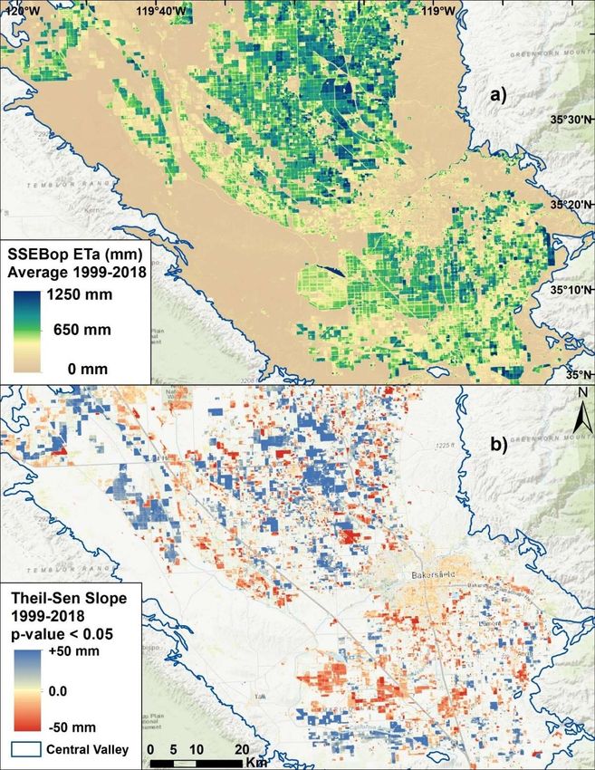
Trend analysis using the MK test on the crop area (as shown in Table 7) confirms the declining
trends in traditional crops in favor of fruit/nut crop types. Cotton shows the sharpest decline with
a statistically significant decrease at a rate of 3589 ha/year. Alfalfa and wheat also see significant, if
smaller, declines in crop area. Smaller crops such as carrots, corn, and potatoes also see statistically
significant decreasing trends in crop area at a rate between 100 and 200 ha/year. However, the fruit/nut
crops all see statistically significant increasing trends over the 20-year period. Almonds increase in area
at a rate of 2465 ha/year and pistachios increase at a rate of 1095 ha/year. Although the total footprint
of pistachios is smaller than that of almonds, their increasing importance in Kern County’s agricultural
production is clear. Grapes and oranges also see statistically significant increases in crop area over
time, although to a smaller extent than nuts.
Table 7. Simple Mann–Kendall trend results for the area of 10 major commodities in Kern County from
1999 to 2018 showing: (1) Mann–Kendall trend statistic, (2) p-value, (3) Theil–Sen slope (in hectares)
from 1999 to 2018, and (4) the significant trend where (+) and (−) indicate statistically significant
increasing or decreasing, respectively, trends where the p-value is less than 0.05 and (#) signifies the
trend is not statistically significant and the p-value is greater than 0.05.
Crop Type MK Statistic p-Value Theil–Sen Slope (ha/yr) 1 Trend 2
Alfalfa −113 0.000 −758 −
Almonds 175 0.000 2465 +
Carrots −101 0.001 −180 −
Corn −62 0.048 −116 −
Cotton −159 0.000 −3589 −
Grapes 123 0.000 358 +
Oranges 109 0.000 227 +
Pistachios 179 0.000 1095 +
Potatoes −71 0.023 −165 −
Wheat −111 0.000 −560 −
1 In hectares (ha). 1 hectare = 2.47 acres, 2 Durbin–Watson statistic shows no serial correlation for the statistically
significant trends.Remote Sens. 2019, 11, 1782 14 of 22
On average, the top 10 crops of Kern County consume 158,312 ha-m of water annually from 1999
to 2018. In the beginning of the study period, cotton is the predominant water user in the county
consuming 26% or 41,075 ha-m of water in 1999 but, as shown in Figure 5, as the crop area for cotton
declines, the water use also declines until cotton is reduced to only 3% of the total crop water use in
2018 at less than 4000 ha-m. The decline in crop water use is directly correlated with the decline in crop
area with an r2 = 0.99. Alfalfa, the second highest consumer of water in 1999, saw a similar reduction
in crop water use as its agricultural footprint receded. Alfalfa consumed 32,015 ha-m of water in 1999,
20% of the total crop water use. However, by 2018, alfalfa was reduced to just over one-third of that
volume (11,095 ha-m) and consumed just over 8% of the total crop water use. Other row crops such as
wheat also experienced a 5% decline in their share of total crop water use. The 2018 water use for wheat
was 86% less than the water used in 1999. Water use by these three traditional row crops was further
reduced during the 2012–2016 California drought. Alfalfa fared the best at only 14% below the 20-year
Remote Sens. 2019, 11, x FOR PEER REVIEW 14 of 22
mean during the drought, but cotton and wheat saw drought reductions of 61% and 38%, respectively.
Figure 5. The top five crops in Kern County from 1999 to 2018 showing the SSEBop ETa mean (in mm)
Figure 5. The top five crops in Kern County from 1999 to 2018 showing the SSEBop ETa mean (in mm)
for the
forUSDA-NASS
the USDA-NASS CDLCDL
cropcrop
type, thethe
type, bias-corrected area
bias-corrected areaestimate
estimate(in
(inhectares),
hectares), water usevolume
water use volume
(ha-m) and the net irrigation (ha-m) in hectare-meters. The area, water use, and net irrigation
(ha-m) and the net irrigation (ha-m) in hectare-meters. The area, water use, and net irrigation are are
scaledscaled by 10,000 (i.e., 4 ha-m corresponds to 40,000 ha-m). 1 hectare = 2.47 acres. 1 hectare-meter ==
by 10,000 (i.e., 4 ha-m corresponds to 40,000 ha-m). 1 hectare = 2.47 acres. 1 hectare-meter
8.1078.107 acre-feet.
acre-feet.
As forAsthe
forfruit/nut
the fruit/nut
cropscrops in Kern
in Kern County,
County, almondsalmonds unsurprisingly
unsurprisingly become
become the heaviest
the heaviest waterwater
user
userCounty
in Kern in Kern asCounty as the agricultural
the agricultural footprint
footprint of almond
of almond production
production expanded.
expanded. Eighteen
Eighteen percentof
percent
total of total
crop crop use
water water
in use
1999inwas1999consumed
was consumed by almonds
by almonds at 29,275
at 29,275 ha-mha-mbutbut
by by 2018,
2018, thethe totalshare
total shareof
crop of crop use
water water usetorose
rose 48% to or
48% or 66,243
66,243 ha-m.ha-m.
ThisThis increase
increase in in cropwater
crop wateruse
useisis directly
directly linked
linkedtotothe the
rise in crop area as the annual area and annual water use for almonds are correlated
rise in crop area as the annual area and annual water use for almonds are correlated with an r = 0.97. with an r 22= 0.97.
Pistachios
Pistachios sawsaw a similar
a similar pattern
pattern as as pistachios
pistachios increased164%
increased 164%in in 2018
2018 from
from the
the 1999
1999total
totalwater
wateruse.use.
This This
shiftsshifts the proportion
the proportion of crop
of crop water
water useuse
forfor pistachiosfrom
pistachios from4% 4%inin1999
1999 up
up toto 13%
13% in in 2018.
2018.Fruit
Fruit
cropscrops
suchsuch as grapes
as grapes showed
showed a more
a more stable
stable pattern
pattern overthe
over the20-year
20-yearperiod.
period. Although
Although grapes grapessaw sawan an
increase in water use from 1999 to 2018, the increase was more subtle with only a 23% increaseinin
increase in water use from 1999 to 2018, the increase was more subtle with only a 23% increase
2018 totals as compared to 2008 with the proportion of total water use shifting 5% during the 20-year
2018 totals as compared to 2008 with the proportion of total water use shifting 5% during the 20-year
period. Oranges showed a similar pattern but even more subtle (see Table 8). Furthermore, unlike the
period. Oranges showed a similar pattern but even more subtle (see Table 8). Furthermore, unlike the
traditional row crops, none of the fruit/nut crops showed a decline in water use during the 2012–2016
traditional row crops, none of the fruit/nut crops showed a decline in water use during the 2012–2016
drought, but instead saw percent deviations that were increased from the 20-year mean.
drought, but instead saw percent deviations that were increased from the 20-year mean.
Table 8. Summary statistics of the crop water use estimates for the top 10 major crops in Kern County
Figure 1999. to 2018 ordered by mean including: (1) the mean of the 1999–2018 period, (2) the crop
area in 1999 and the percentage of the total crop area, (3) the crop area in 2018 and the percentage of
the total crop area, (4) the change in crop area between 1999 and 2018, and (5) the mean crop area
during the 2012–2016 California drought and percent deviation from the mean.
1999 Water Use 2018 Water Use
Crop Type Mean Water Use (ha-m) 1 % Change 2012–2016 Drought (ha-m) 1 [%]
(ha-m) 1 [%] (ha-m)1 [%]You can also read


