Too Young to Leave the Nest? The Effects of School Starting Age
←
→
Page content transcription
If your browser does not render page correctly, please read the page content below
INSTITUTT FOR SAMFUNNSØKONOMI
                                                                                       DEPARTMENT OF ECONOMICS

SAM 11 2008
ISSN: 0804-6824
JUNE 2008

      Discussion paper

      Too Young to Leave the Nest?
      The Effects of School Starting Age

      BY
      SANDRA E. BLACK, PAUL J. DEVEREUX, AND KJELL G. SALVANES

      This series consists of papers with limited circulation, intended to stimulate discussion.
Too Young to Leave the Nest?
*
The Effects of School Starting Age
by
Sandra E. Black
Department of Economics
UCLA, IZA and NBER
sblack@econ.ucla.edu
Paul J. Devereux
School of Economics and Geary Institute
University College Dublin, CEPR and IZA
devereux@ucd.ie
Kjell G. Salvanes
Department of Economics
Norwegian School of Economics
Statistics Norway
Center for the Economics of Education (CEP) and IZA
kjell.salvanes@nhh.no
April 2008
*
Black and Devereux gratefully acknowledge financial support from the National
Science Foundation and the California Center for Population Research. Salvanes thanks
the Research Council of Norway for financial support. We would like to thank seminar
participants at UCD Geary Institute, the ESRI, the University of Maryland, Irvine, Davis,
and the Tinbergen Institute. We are indebted to Stig Jakobsen who was instrumental in
obtaining data access to the IQ data from the Norwegian Armed Forces.
1Abstract
Does it matter when a child starts school? While the popular press seems to
suggest it does, there is limited evidence of a long-run effect of school starting age on
student outcomes. This paper uses data on the population of Norway to examine the role
of school starting age on longer-run outcomes such as IQ scores at age 18, educational
attainment, teenage pregnancy, and earnings. Unlike much of the recent literature, we are
able to separate school starting age from test age effects using scores from IQ tests taken
outside of school, at the time of military enrolment, and measured when students are
around age 18. Importantly, there is variation in the mapping between year and month of
birth and the year the test is taken, allowing us to distinguish the effects of school starting
age from pure age effects. We find evidence for a small positive effect of starting school
younger on IQ scores measured at age 18. In contrast, we find evidence of much larger
positive effects of age at test, and these results are very robust. We also find that starting
school younger has a significant positive effect on the probability of teenage pregnancy,
but has little effect on educational attainment of boys or girls. There appears to be a
short-run positive effect on earnings of beginning school at a younger age; however, this
effect has essentially disappeared by age 30. This pattern is consistent with the idea that
starting school later reduces potential labor market experience at a given age for a given
level of education; however, this becomes less important as individuals age.
2Does it matter at what age a child starts school? Older children do better on tests,
but is this because they are older and, in fact, unrelated to the age they started school?
Despite the dearth of convincing evidence, the popular press seems to suggest that there
are benefits to “redshirting” (holding back) children in kindergarten (See NY Times, June
3, 2007). But is this the case? Are the short run benefits in terms of better performance
just that: short run? And are there costs associated with finishing school and starting
work later?
Much research has shown a consistent pattern that children who start school later
tend to score higher on in-school tests, even after accounting for the endogeneity of
school starting age.1 However, a key limitation in the interpretation of these correlations
is the inability to distinguish between the effect of school starting age and a direct age-at-
test effect, as they are perfectly collinear. As a result, it could be that children who start
school when they are older do better simply because they are older when they take the
tests and being older provides an advantage, or it could be because there are direct
benefits to starting school at an older age.
Using data on the population of Norway, we are able to separate these two effects
using IQ test scores measured outside of school, at the time of military enrolment when
students are around age 18. The rule in Norway that children must start school the year
they turn 7 provides a discontinuity in school starting age for children born around
January 1st and provides an instrument for actual school starting age. Importantly, there is
also variation in the mapping between year and month of birth and the year the test is
1
This includes a cross-country study by Bedard and Dhuey (2006) and country-level studies by Fredrikson
and Ockert (2006) for Sweden, Puhani and Weber (2007) for Germany, Strom (2004) for Norway,
Crawford, Dearden and Meghir (2007) for England, McEwan and Shapiro (2008) for Chile, and Elder and
Lubotsky (2007) for the US.
3taken, allowing us to distinguish the effects of school starting age from pure age effects.
Cognitive scores around age 18 are particularly interesting as it is about the time of entry
to the labor market or to higher education and so these scores are more relevant to the
labor market than scores in kindergarten or elementary school.
Additionally, we study the effects of school starting age on longer term outcomes
including educational attainment, early fertility, and adult earnings. While this is
methodologically less complicated than studying in-school tests because age of
measurement and school starting age are not perfectly collinear, the literature has been
hindered by a paucity of data. Given the complications created by school leaving age
rules in the US, European data are attractive when studying education and earnings.2
Educational attainment has been studied in the literature and it has generally been found
that older starters average modestly higher completed education.3 However, ultimately
adult earnings are a very important outcome and we add to the literature by being the first
study to track cohorts of men and women from ages 24 to 35 and analyze how the
impacts of school starting age change with age. Also, we are the first study to examine
the effects of school starting age on the probability of teenage childbearing by women.
There has been some more recent evidence that the timing of births may be
manipulated by parents based on school starting age cutoffs; to the extent that this is true
and that these parents may be “different” on other dimensions as well, estimates in the
2
Studies using U.S. data have suffered from the fact that compulsory schooling laws specify minimum
school leaving ages rather than grades so early starters have completed more education at the minimum
dropout age. Therefore, historically, persons whose quarter of birth predicts starting early have on average
higher schooling and higher earnings (Angrist and Krueger 1991). Dobkin and Ferreira (2007) finds
younger starters also obtain slightly higher education in more recent U.S. cohorts.
3
See Puhani and Weber (2007) and Fertig and Kluve (2005) for Germany, and Fredrikson and Ockert
(2006) for Sweden.
4literature may be biased. Unlike the previous literature, we can control for sibling fixed
effects to take account of this possibility.
There are a number of reasons why school starting age may have long-run effects
on children’s outcomes, although the sign of this effect is theoretically ambiguous. The
potential advantages of an early starting age could include the following: Starting school
younger means finishing school at a younger age, which implies more time for the
individual to earn returns on their investment in human capital. Starting school younger
may also be advantageous to the extent that children learn more at school than at home
(or be a disadvantage if the opposite holds true), which could affect their long run
trajectory. Finally, parental investment in their children may also depend on school
starting age – parents may provide more help to children who are young for their grade
level.
There are also potential disadvantages of an early starting age (and some of these
could work in the opposite direction as well). It is possible that children cannot learn as
well in school earlier in their developmental life. In addition, social development may
depend on a child’s age relative to that of his/her classmates; if being relatively older is
advantageous, then it might be better to start children later (and vice versa). To the extent
that older children have an advantage on exams in school (by mere virtue of the fact that
they are older when they take the test and hence know more), they may do better in the
long run. Given these potentially offsetting effects, the true causal relationship becomes
an empirical question.
We find evidence for a small positive effect of starting school younger on IQ
scores measured at age 18. In contrast, we find evidence of much larger positive effects
5of age at test, and these results are very robust. When we examine other outcomes, we
find that school starting age has a significant effect on teenage pregnancy among girls but
no strong effect on education among girls or boys. We also find that there appears to be a
short-run positive effect on earnings of beginning school at a younger age; however, this
effect has essentially disappeared by age 30. This pattern is consistent with the idea that
starting school later reduces potential labor market experience at a given age for a given
level of education; however, this becomes less important as individuals age.
The paper unfolds as follows. Section 2 presents the relevant literature. Section 3
describes our methodology and contrasts it to other approaches in the literature. Section 4
discusses relevant institutional details in Norway, and Section 5 provides a data
description. Section 6 presents our results and Section 7 concludes.
2. Relevant Literature
Despite the importance of the distinction, there is little solid evidence as to the
role of school starting age (SSA) versus test age (AGE) in determining school test scores.
While children are in school, researchers are faced with the identity that
AGE AT TEST = SCHOOL STARTING AGE + YEARS OF SCHOOLING
Most of the literature has compared test scores of children who are in the same grade and
so has in fact estimated the combined effects of SSA and AGE.
Given the difficulty with separating out the two effects, a number of recent papers
try to infer the role of age versus school starting age by looking either at early test scores
or at changes in scores over time.4 Elder and Lubotsky (2007) show that there are strong
4
For example, Datar (2006) finds that achievement changes between kindergarten and first grade are not
highly correlated with age at school entry.
6age effects in the fall of kindergarten year, before children could have been much
affected by formal schooling. Elder and Lubotsky (2007) and Cascio and Schanzenbach
(2007) also show that effects of age-at-school-entry on test scores tend to get smaller as
children move to higher grades. Together these papers imply that the estimated starting
age effects partly reflect the endowment differences between students when school starts
and that there is little evidence that students learn more in school if they are older when
they start. However, none of this work is able to directly disentangle the direct effect of
age at test from that of school starting age.
While most of the literature controls for time in school, there is another series of
papers that controls for age at test. There is some evidence that, when tested at the same
age, young children score better on in-school tests if they started school younger and
hence have spent more time in school. Cahan and Cohen (1989) study Israeli elementary
school children and Elder and Lubotsky (2007) compare U.S. children around age 6 but
with different predicted starting ages (based on month of birth). However, the bulk of this
evidence is for very young children in kindergarten and elementary school and it is not
clear that these findings generalize to older ages relevant to the labor market
Most similar methodologically to this paper are papers by Crawford, Dearden and
Meghir (2007) and Cascio and Lewis (2006), both of which rely on multiple sources of
variation to identify the effect of school starting age on children’s test scores. Crawford,
Dearden and Meghir (2007) use the fact that there is variation in school starting age
across local education authorities (LEAs) in Britain to separately identify the effect of
school starting age from age at test effects on in-school tests. While some LEAs have
only one entry point (with one cutoff date), other LEAs have two entry points (with some
7children starting in September and some starting in January) or even three entry points
(with children starting school in September, January, and April). So while the school
start cutoff in Britain is September 1st, August-born children start school in September in
some LEAs and later in the year in others. Thus, the effect of SSA can be distinguished
from that of test age by comparing August and September born children who are in LEAs
that have different policies. They find that age at test is the biggest factor; however, a
limitation of this methodology is that the different school starting policies may
themselves be disruptive or lead to changes in curriculum and so may impact both August
and September born children.5
Cascio and Lewis (2006) examined the role of schooling on student performance
on the Armed Forces Qualifying Test (AFQT) in the NLSY. A nice feature is that it
focuses on older children and there is variation in school cutoff ages (arising from across
state variation) as well as variation in the age at which individuals take the test. This
suggests that the authors are able to identify the effect of school starting age while
controlling for age (they actually interpret these estimates as effects of schooling but as
described above, schooling and school starting age are perfectly collinear for in-school
children, conditional on age). Unfortunately, likely due to a relatively small sample, the
authors find very imprecise statistically insignificant effects of school starting age when
controlling for age. Because we have data on the population of Norway, we are much
better able to identify the effect of school starting age controlling for age.6
5
Another limitation of this paper is that the authors know the LEA a child is in at the time of the exam, not
when they started school, suggesting that results for the earliest tests scores may be most valid.
6
Mayer and Knutson (1999) also find some evidence that quarter of birth matters for test scores in the
CNLSY.
8There is also a recent literature examining the relationship between school starting
age and longer run outcomes such as educational attainment and earnings.7 While
methodologically this is less complex because there is no link between date of
measurement and time in school, the literature has been limited by the absence of good
data. For example, the most thorough previous study of earnings by Fredrikson and
Ockert (2006) has only one year of earnings data and so cannot distinguish between
cohort and age effects. We are the first study to track cohorts of men and women from
ages 24 to 35 and analyze how the impacts of school starting age change with age.
3. Methodology
Identification Strategy
We first describe the empirical strategy we use when our outcome variable is
completed years of education, log earnings, or probability of having a teenage birth. We
then describe the adjustments we make when we look at IQ as an outcome; as described
earlier, when we look at IQ we need to account for the fact that we control for age at test.
Education, Log Earnings, and Teenage Fertility Outcomes
Our equation of interest is as follows:
Yi = β 0 + β1 SSAi + X i ' λ + ε i (1)
where Y is the outcome under study, SSA is the school starting age, and X is a vector of
controls that includes year of birth indicators and a local linear trend. Because the school
cutoff is at the beginning of the year, we redefine year of birth to run from July to June
rather than from January to December (so the discontinuity is now at the middle of our
7
Bedard and Dhuey (2007) use variation in school starting age within states over time in the United States
to identify the effect of cohort age and absolute age (netting out relative age effects). Their findings
suggest a significant positive effect of increasing the school starting age on wages.
9re-defined “year”).8 We also include a local linear trend that is centered at the
discontinuity (a trend ranging from 1-12 and centered at December/January). Together
the year of birth indicators and local linear trend allow for cohort effects such as secular
increases in educational attainment over time.
Because parents may be able to manipulate school starting age, we need to find an
instrument to identify the true relationship between school starting age and outcomes.
Our exogenous variation in school starting age comes from variation in month of birth
and the administrative school starting rule in Norway – children born in December start
school a year earlier than children born in January, with a December 31 cutoff. Therefore,
we estimate equation (1) by 2SLS using the expected school starting age (ESSA) as an
instrument for the actual school starting age. In Norway during our sample period, the
legal rule was that children must start school in the year they turn 7. We measure the
ESSA as equal to 7.7 – (month of birth -1)/12. This takes account of the fact that school
starts in August and the cutoff date is at the beginning of the year. Given the ESSA is
determined only by month of birth and not by parental choice, it seems reasonable to treat
it as exogenous and use it as an instrument for the actual SSA.
For ESSA to be a valid instrument for SSA, two conditions must be satisfied.
First, it must be random which children are born in different months of the year; this
could be violated if different types of families have children at different times of the year.
We attempt to address this issue in a number of ways. As a robustness check, we include
family characteristics in our regression and show our resulting estimates are very close to
those estimates without these controls. In addition, and perhaps more convincing, we are
also able include family fixed effects as a check on this possibility.
8
Fredrikson and Ockert (2006) also use this redefined-year approach in their Swedish study.
10Second, it must be that there is no direct effect of being born at a particular time
of the year on child outcomes. While there is some evidence of small differences in
health outcomes across season of birth (Bound and Jaeger 2000), the balance of previous
evidence is that these differences are not nearly large enough to make much difference.
Importantly, our critical comparison is between December- and January- born children,
so differences between summer and winter born children are largely irrelevant.
It is important to note that the thought experiment here is that we vary one
individual’s school starting age while holding that of everybody else fixed. Thus, we are
essentially changing two things: the age the individual starts school and the relative age
of that child in the classroom (from relatively younger to relatively older). Given that we
have no information on variation in the ages of other children in the class, we cannot tell
whether our estimated effect of starting a year later matters because it makes the child a
year older in absolute terms or because it makes the child older relative to his classmates.
IQ Scores as Outcomes
As described previously, when we study IQ scores at age 18, we add a control for
the age of the person at the time of the test (AGE):
IQi = β 0 + β1 SSAi + β 2 AGEi + X i ' χ + ε i (2)
In Norway, there is a relationship between month of birth and when persons are called to
do the test. As an example, in some years, individuals who were born in January and
February are called to take the exam in one year while individuals born after February (in
the same year) are called to take the exam a year later. Since in most years, the birth
month cutoff for the test is not December and so is not perfectly correlated with expected
11school starting age, we are able to disentangle school starting age effects from general
age effects.
A complication that arises is that not all men take the test in the year in which
they are supposed to do so. This type of deviation can occur due to illness, absence
abroad etc. As a result, age at the time of the exam is potentially endogenous.
Conceptually similar to the case of school starting age, we use the year in which you
were supposed to take the test as an instrument for the age at which did take the test. To
do so, we define test feeder groups for each test year based on year and month of birth.
For example, all persons born in calendar year 1951 were supposed to take the test in
1970, so they are all members of the 1970 feeder group. On the other hand, persons born
between April 1961 and April 1962 were supposed to take the test in 1980, so they
constitute the 1980 feeder group. We instrument for AGE using the indicator variables
for the feeder group to which each individual belongs. This exploits the discontinuity that
while cohort of birth changes smoothly, persons born in April 1961 are almost a year
older taking the test than persons born in March 1961. Given that over 90% of men do the
test in the year they are supposed to, the first stage relationships are extremely strong and
there is no concern about weak instruments.
Appendix Figure 1 illustrates the discontinuity between test month cutoff and age
at test in our data. In the figure, zero corresponds to cutoff birth months and -1 to birth
months that are one month previous to a cutoff birth month etc. The figure shows how
average age at test varies depending on where the person’s birth month is relative to the
relevant cutoff birth month for that individual. The very large discontinuity in age at test
at the cutoff birth months is very clear.
12As described earlier, conditional on age, school starting age is typically perfectly
correlated with time-in-school when the outcome is measured while still in school. In
Norway, many boys take the military IQ tests while still in school; our estimates for IQ
will therefore provide an upper bound on the benefits of starting school young, holding
schooling constant. Later we evaluate the role played by time-in-school by providing
separate estimates for persons who had finished schooling by the time of the test.
Additional Specifications
In addition to the 2SLS procedure described above, we also estimate two
additional specifications for all our outcomes:
Discontinuity Sample
The specification in equations (1) and (2) uses all months for identification of the
SSA effect but allows other factors to impact IQ scores smoothly (linearly) through the
discontinuity point.9 As a robustness check, we also estimate our equation on the
subsample of individuals born in either December or January, thereby using only the
individuals born close to the discontinuity for identification. In this case, the local linear
trend is unidentified and so is excluded from the estimating equation. The assumption
underlying use of the discontinuity sample is that December and January observations are
exchangeable so that, on average, their outcomes differ only because of the difference in
their school starting ages.
Family Fixed Effects
There has been some recent evidence that the timing of births may be manipulated
by parents based on school starting age cutoffs; to the extent that this is true and that
9
Note that, even using all months, the discontinuity in ESSA is necessary for identification as, in the
absence of the jump in January, ESSA would be perfectly correlated with the linear trend.
13these parents may be “different” on other dimensions as well, our estimates may be
biased.10 However, because we have data on the population of Norway, we can also
investigate the relationship between school starting age and long run outcomes within
families, thereby differencing out any time-invariant family qualities. To do so, in some
specifications we estimate the 2SLS regressions with additional dummy variables for
each set of siblings. These specifications will provide consistent estimates unless the
timing of births amongst siblings is correlated with the counterfactual outcomes of the
children. This seems unlikely as child endowments are not known before birth but could
arise if, for example, parents decide to strategically time the second child in response to
indications that the first child was low quality.
4. The Norwegian Childcare and School System
In Norway, children under the age of seven can be placed in a daycare facility;
Norway has both public and private facilities. However, prior to the mid 1970s, labor
market participation rates for married women were relatively low, with rates in the 35%
range in the 1960s and in the 40% range in the early 1970s. In addition, families faced a
shortage of daycare facilities during that period. As a result, prior to 1980, daycare
enrollment for children between the ages of 3-6 was around 10 percent or less, with a
large increase during the 1980s.11
In the late 1970s through the 1980s, there was a large increase in labor force
participation rates of married women, to over 70 percent by 1990. This was accompanied
by a larger increase in preschool enrollment. The expansion that began in the 1980s
10
See Crawford, Deardon, and Meghir (2007).
11
Up to 1980, most daycare facilities were located in urban areas and most catered to the children of
working mothers.
14represented a particularly sharp increase in coverage in rural areas. Appendix Table 1
shows preschool coverage by age of child from 1963-2002. (Source: Pettersen, 2003).
While our data broadly cover children aged 6 between 1968 and 1994, most of our
outcomes rely on children born in the earlier part of the period. This suggests that, during
the time period relevant to our sample, most children were at home prior to enrollment in
school, either with their mother or an informal childcare provider such as a grandparent
or a neighbor.
In terms of schooling, all compulsory education in Norway is free. Since 1997,
schooling has been compulsory from age 6 to 16 (10th grade). However, the cohorts we
consider faced a school starting age of 7 and 9 years of compulsory schooling (until age
16). Schools are generally run by the local Municipality and there is no streaming by
ability during the years of compulsory schooling.12
Norway has mandatory military service of between 12 and 15 months (fifteen in
the Navy and twelve in the Army and Air Force) for men between the ages of 18.5 (17
with parental consent) and 44 (55 in case of war). However, the actual draft time varies
between six months and a year, with the rest being made up by short annual exercises.
Students have tended to attend university after completing military service with the result
that average age of college students is 22 in Norway (Mortimore et al, 2004).
5. Data
Our primary data source is the Norwegian Registry Data, a linked administrative
dataset that covers the population of Norwegians up to 2006 and is a collection of
different administrative registers such as the education register, family register, and the
12
There are very few private schools in Norway and only about 2% of all pupils attend them.
15tax and earnings register. These data are maintained by Statistics Norway and provide
information about educational attainment, labor market status, earnings, and a set of
demographic variables (age, gender) as well as information on families.13 To ensure that
all individuals studied went through the Norwegian educational system, we include only
individuals born in Norway. We have information on school starting age for cohorts born
from 1962 onwards and our analysis focuses on the 1962-88 cohorts.
The IQ data are taken from the Norwegian military records from 1980 to 2005. In
Norway, military service is compulsory for every able young man. Before entering the
service, their medical and psychological suitability is assessed; this occurs for the great
majority between their eighteenth and twentieth birthday. IQ at these ages is particularly
interesting as it is about the time of entry to the labor market or to higher education.
The IQ measure is a composite score from three speeded IQ tests -- arithmetic,
word similarities, and figures (see Sundet et al. [2004, 2005] and Thrane [1977] for
details). The arithmetic test is quite similar to the arithmetic test in the Wechsler Adult
Intelligence Scale (WAIS) [Sundet et al. 2005; Cronbach 1964], the word test is similar
to the vocabulary test in WAIS, and the figures test is similar to the Raven Progressive
Matrix test [Cronbach 1964]. The composite IQ test score is an unweighted mean of the
three subtests. The IQ score is reported in stanine (Standard Nine) units, a method of
standardizing raw scores into a nine point standard scale that has a discrete
approximation to a normal distribution, a mean of 5, and a standard deviation of 2.14 We
have IQ scores on about 84% of the relevant population of men in Norway.15 16
13
See Møen, Salvanes and Sørensen [2004] for a description of these data.
14
The correlation between this IQ measure and the WAIS IQ has been found to be .73 (Sundet et al., 1988).
15
Eide et al (2005) examine patterns of missing IQ data for the men in the 1967-1987 cohorts. Of those,
1.2 percent died before 1 year and 0.9 percent died between 1 year of age and registering with the military
16In terms of educational attainment, we measure education at the oldest age
possible for each individual i.e. in 2006.17 To get as close as possible to completed
education, we do not include anyone in the education sample who is aged less than 27 in
2006.
In terms of teenage childbearing, we study two related outcome variables. The
first is whether a woman has a child as a teenager, and the second is whether a woman
has a child within 12 years of her expected school starting age. While the former is the
more standard measure of teenage childbearing, the latter is plausibly a better measure of
whether early motherhood is likely to disrupt human capital accumulation and hence later
earnings potential. Given that most of our sample completes at least 12 years of schooling
and 12 is the modal level of schooling, this outcome variable measures whether women
are likely to find it difficult to obtain the normal level of education because they have
children.
We construct the first variable by restricting the sample to women aged at least 36
in 2006 and denoting a teen birth if they have a child that is aged at least 16 in 2006 who
was born before the woman was aged 20.18 The second dependent variable is constructed
at about age 18. About 1 percent of the sample of eligible men had emigrated before age 18, and 1.4
percent of the men were exempted because they were permanently disabled. An additional 6.2 percent are
missing for a variety of reasons including foreign citizenship and missing observations. There are also
some missing IQ scores for individuals who showed up to the military.
16
One concern is that missing IQ is nonrandom and is related to SSA. To examine this, we regressed an
indicator whether IQ is missing on SSA using the standard specification; while the OLS results are positive
and significant, 2SLS estimates were small and insignificant. We got similar results when we examined
missing earnings.
17
Our measure of child educational attainment is reported by the educational establishment directly to
Statistics Norway, thereby minimizing any measurement error due to misreporting. This educational
register started in 1970. See Møen, Salvanes and Sørensen [2004] for a description of these data.
18
This sample restriction is required because to know whether a woman had a teen birth we need to see
whether or not a child appears in the panel with whom she has a less than 20 years age gap. The effect is
that the cohorts we use are born between 1963 and 1969.
17using the same sample. On average in our sample, 8% of women have a birth as a
teenager and 6% have a birth within 12 years of the expected school start date.
Finally, earnings are measured as total pension-qualifying earnings reported in the
tax registry and are available from 1986 to 2005. These are not topcoded and include
labor earnings, taxable sick benefits, unemployment benefits, parental leave payments,
and pensions.
For the purposes of studying earnings and employment, we restrict attention to
individuals aged between 24 and 35. In this group, about 94% of both men and women
have positive earnings. Given this high level of participation, our first outcome is
log(earnings) conditional on having non-zero earnings. Since the results for this variable
encompass effects on both wage rates and hours worked (and since the earnings measure
picks up earnings from summer work by students and other short-term activity), we also
study the earnings of individuals who have a strong attachment to the labor market and
work full-time (defined as 30+ hours per week). To identify this group, we use the fact
that our dataset identifies individuals who are employed and working full time at one
particular point in the year (in the 2nd quarter in the years 86-95, and in the 4th quarter
thereafter).19 We label these individuals as full-time workers and estimate the earnings
regressions separately for this group. About 52% of our male sample are employed full
time aged 24 but this increases to 78% by age 35. The equivalent figures for women are
42% and 50%.
Table 1 presents summary statistics for our sample.
19
An individual is labeled as employed if currently working with a firm, on temporary layoff, on up to two
weeks of sickness absence, or on maternity leave.
186. Results
First Stage Estimates
In Norway during our sample period, the legal rule was that children must start
school in the year they turn 7. In practice, compliance with this rule was almost perfect
for the cohorts we study. (Appendix Table 2 shows compliance rates by birth year for
cohorts born 1962-1988.)20 This is not surprising as parents had to formally apply for an
exception from the rule and the application had to be approved by health and school
specialists as well as by the local government (Strom 2004). The high compliance rates
are reassuring as they imply that our IV estimates can be interpreted as an approximation
to the average treatment effect of school starting age rather than the usual LATE
interpretation.21
We report first stage estimates by gender in Table 2 for the full sample and for the
discontinuity sample. Because the first stage estimates are quite similar across the
particular samples used for different outcomes, for parsimony we have chosen to report
first stages for the full set of cohorts born between 1962 and 1988. Using the full sample,
the first stage coefficient on ESSA is .80 for men and .82 for women. These change very
little when family fixed effects are added to the specification in column (3).
As one might expect, compliance rates are lower for children born in December
and January than for persons born during the middle of the year (see Appendix Table 3).
This can be seen in the lower first stage estimate for ESSA when the discontinuity sample
20
Bedard and Dhuey (2006), using TIMMS data, show that in 4th grade only 2% of Norwegians are not in
the predicted grade given their month of birth and Strom (2004) reports that 99.5% of the 1984 cohort of
Norwegian public school students in the 2000 PISA are in grade 10 (as they should be).
21
Consistent with recent popular press, we find that it is the better educated mothers who are more likely to
be noncompliers; however, counter to this anecdotal evidence on “redshirting”, these mothers are actually
more likely to start their children early. (“When Should a Kid Start Kindergarten?” New York Times, June
3, 2007)
19is used (see column (2) of Table 2). However, even in this sample, the first stage
estimates are about .75.
IQ Results
Our results for IQ test scores are presented in Table 3 (we have this information only for
men). We first present the OLS results (Column 1), which suggest that SSA has a large
negative effect on military test scores. The coefficient of -.8 implies that going to school
one year later reduces test scores by 4/5 of a stanine or almost half a standard deviation.
In contrast, the OLS estimates suggest no impact of age at test, which runs counter to our
prior that older boys score higher on tests. Of course, the OLS estimates may be
suffering from selection bias, with less-able children having their school entry, and
possibly their test-taking, delayed.
To address this issue directly, from this point forward we treat SSA and age at test
as endogenous and use the 2SLS strategy described previously. In contrast to the OLS
results, the 2SLS estimates show a strong positive effect of age at test on IQ. The
estimate implies that being one year older when taking the test increases the score by
about .22; this is one fifth of a stanine and about one tenth of a standard deviation.
Additionally, the effect of SSA is still negative and statistically significant but is much
smaller, suggesting that starting school a year later reduces IQ scores by about .06, about
one twentieth of a stanine.
Taken together, the age-at-test and SSA coefficients provide a prediction of what
one would obtain if a boy started school a year later and, as a result of taking the exam
with his school entry cohort, took the exam a year later. In this case, the estimated SSA
20effect would be the sum of the true SSA effect and the age-at-test effect. This equals .16,
which is about 8% of a standard deviation. This is somewhat lower than the findings in
the literature that use in-school tests (for example, using 9th grade GPA in Sweden,
Fredriksson and Ockert find a positive effect of SSA that is about 20% of a standard
deviation). The smaller effect is unsurprising given that our test-takers are older and that
the IQ tests probably measure fixed components of intelligence to a greater extent than
in-school tests.
Robustness checks
In Columns (3) and (4) in Table 2, we investigate the robustness of our 2SLS
estimates to alternative specifications. In Column 3, we focus specifically on individuals
who are born in the months of December or January and hence are right around our point
of discontinuity. By restricting the sample, it is clear where our identification is coming
from. As expected, the sample size is greatly reduced and, though consistent with our
earlier findings, the results are less statistically precise.
Finally, the fourth column includes family fixed effects estimates and controls for
the birth order of the child. The number of observations is lower for these specifications
because we exclude families in which there are not at least two boys with IQ scores.
Again, the results are quite robust to using even within-family differences for
identification. Apparently, there are no serious biases arising because of strategic birth
timing by parents.
In Appendix Table 4 we report a set of alternative specifications to reassure that
our findings are robust to specification. These include allowing the local linear trend to
21be different for each birth year, including a quadratic local trend, allowing the local linear
trend to change slope after January, including a quartic in cohort defined at the monthly
level, and including controls for maternal education, birth order, and family size. None of
these specifications provide appreciably different estimates and so we will focus on the 4
specifications in Table 3 for the remaining outcomes.22
Is the SSA effect a time-in-school effect?
While the test is not administered in school (and is, in fact, unrelated to
schooling), there are many individuals in our sample who have not finished schooling at
the time of the test. In this case, the estimated school starting age effect will encompass
the fact that later starters have spent less time in school (since, for example, among
individuals who ultimately complete college, those who started a year later will have not
only a later school starting age but one year less of education at the time of the test.)23 To
test the sensitivity of our results to this, we break our sample into those who, ex post,
actually were finished with their schooling at the time of the test (i.e. those who have ten
or fewer years of education in 2006) and those who have not completed their education at
the time of the test (i.e. those who have at least twelve years of education in 2006).24
One potential problem with this approach is that completed education may be
endogenous because SSA influences educational attainment. However, as we will see in
22
While we do not report them, we have carried out similar specification checks for the other outcomes and
found those estimates to be similarly robust to specification.
23
Leuven et al. (2006) find little evidence that time in school matters for Dutch Kindergarten children.
24
Among those who ultimately completed 12 years of education, we are observing a mix of those who did
and did not complete their education at the time of the test – in almost all cases, persons with 12 years of
education who are born in January and so start school late had not finished schooling at the time of the test.
22the next section, there is no evidence in our data that educational attainment of men is
affected by SSA.
These results are presented in Columns 5 and 6 in Table 3. When we restrict the
sample to cases where both early and late starters are finished education by the time of
the test, we get no statistically significant effect of school starting age and a slightly
smaller (but still statistically significant) effect of age at test. Given that we have found
relatively small effects of SSA on IQ in earlier specifications, this is consistent with even
these small effects being largely explained by the fact that early-starters have more
schooling at the time of the test (given that effect goes away in the sample where those
with an earlier starting age have no education advantage). The estimates also suggest that
a small proportion of the estimated age effect is actually a time-in-school effect.25
Other Outcomes
We are also able to examine the role of school starting age on a number of other
longer-run outcomes. These include education, earnings, and teenage childbearing.
Education
There are a number of mechanisms through which school starting age can affect
educational attainment. Costs and benefits of schooling may vary with SSA as they are
influenced by how effectively skills are being learned in school. For example, to the
extent that older children may do better in school, this could have positive spillover
effects onto educational attainment. On the other hand, because later starters will be older
25
Note that we are attributing the difference in the estimated effect of SSA to time in school and not to
heterogeneous treatment effects by educational attainment.
23at any educational level, their time horizon to recoup educational investments will be
shorter and this will tend to depress demand for education.
In the returns to education literature, Angrist and Krueger (1991) first used
quarter of birth (as a proxy for school starting age) as an instrument for educational
attainment acting through compulsory schooling legislation. (Students had to remain in
school until a certain age; those who started school younger would have more schooling
at the time of dropping out.) However, in the Norwegian case, compulsory schooling is
based on years of school completed and not age, so this is not relevant.
Table 4 presents the education results separately for men and women. As with
IQ, Column 1 has OLS results, Column 2 has 2SLS estimates using the full sample,
Column 3 has 2SLS estimates using the December and January subsample, and Column 4
has 2SLS estimates with family fixed effects and birth order controls.
For men, the OLS estimates are strongly negative. However, as before with IQ,
there is little evidence of a causal effect of school starting age on educational attainment
for men, with 2SLS estimates being very small and statistically insignificant in both the
full and discontinuity samples. The only significant effect of SSA for men is in the family
fixed effects specification which shows a negative effect of -.06. This is not a large effect
as it implies that starting a year later reduces education by one year for about one person
in twenty.
The results for women are quite similar. The OLS effect of SSA is large and
negative but the 2SLS specifications give small and statistically insignificant effects. The
exception is that the estimate from the discontinuity sample is statistically significant at
.07 (.03). While this is positive, it is still of modest size. Overall, the evidence for men
24and women suggests that SSA has at best very small impacts on completed years of
education.26
Timing of First Birth
Motherhood at young ages has been associated with many long-term economic
and health disadvantages such as lower education, less work experience and lower wages,
welfare dependence, lower birth weights, higher rates of infant mortality, and higher rates
of participation in crime (Ellwood, 1988; Jencks, 1989; Hoffman et al., 1993; Kiernan,
1997). There is an ongoing debate as to the extent that these adverse effects of teen
childbearing are truly caused by having a teen birth rather than reflecting unobserved
family background differences. (See Hotz, McElroy, Sanders 2005 for an example).
However, as a policy matter, efforts to reduce the rate of teen childbearing are often
considered as a strategy to improve the life chances of young women.
There are at least three reasons we might expect early fertility to be impacted by
school starting age. First, since it is likely to be quite costly to be in school as a young
mother, starting school later may be associated with a postponement of fertility. This has
been called the “incarceration effect”; while women are in school, they do not have the
desire/time/opportunity to have a child. Second, since education increases human capital,
additional schooling may make you “smarter” and hence decide to postpone childbearing;
this might imply that later starters (who have less education at any particular age) are
more likely to have children at a given age.27 Finally, it is likely that a major effect of
26
We have also studied whether the individual has at least 12 years of schooling as the outcome variable
and found very similar results.
27
Black, Devereux, Salvanes (2008) discuss these mechanisms in the context of the effects of compulsory
schooling laws on teenage fertility.
25starting school young is that the child’s peer group is older than it would otherwise be.
Therefore, young starters may be more likely to engage early in adult-type behaviors such
as drug taking and sex.28 While we don’t observe these behaviors directly, childbearing at
young ages signals sexual activity.
The first panel of Table 5 presents the results for the indicator whether or not a
girl had a birth as a teenager (less than 20 years old) and the second panel presents the
results for the indicator whether she had a birth within 12 years of her expected school
starting age. The OLS estimates suggest a small positive effect of SSA on teen
childbearing. However, when we use 2SLS, we find a statistically significant negative
effect of school starting age on teenage pregnancy for both the full sample and the
discontinuity sample, and the coefficient is about -.018 in both specifications.29 This
implies that a three month increase in school starting age reduces the probability of
teenage pregnancy by approximately 0.5 (.25*.018*100) percentage points. While the
family fixed effects estimate is smaller at -.008, it should be noted that it is quite
imprecisely estimated, with the standard error of .008.
When we instead consider the effect on the probability of having a birth within 12
years of the expected school start, the OLS effect of SSA is .019 (.002). The 2SLS effects
of SSA are also positive and even larger: about .04 - .05. A three month increase in
school starting age will increase the probability of a birth within the first 12 years of
school by about 1.2 (.25*.05) percentage points. The family fixed effects estimate is also
28
This argument is similar to that of Argys et al. (2006) who suggest that higher birth order children are
more likely to engage in risky behaviors at young ages because they are influenced by their older siblings.
Also, Black, Devereux, and Salvanes (2005) find that higher birth order women in Norway are more likely
to have births as teenagers.
29
We have verified that the average derivatives of the reduced forms from probit models are very similar to
the linear probability estimates and have similar sized standard errors.
26about this size. The main reason for this large positive effect is that, 12 years after the
ESSA, January-borns are almost one year older than December-borns and age is a prime
determinant of fertility. Our estimates suggest that, although starting school older does
reduce teenage pregnancy, it still increases the probability that a girl will interrupt her
schooling to have a baby.
Earnings
For simplicity, assume that earnings depend on (1) labor supply, and (2) the wage
rate. At age 24, some Norwegians are still in full time education and performing little
paid work. Thus, at these young ages, labor supply differences are particularly important.
Because early starters tend to finish schooling a year earlier, this is a major reason they
should have higher earnings at young ages. At older ages (late 20s on) most individuals
are working so differences in wage rates are probably the dominant reason for earnings
differences. Since wages depend on human capital, they depend on skills acquired up to
the end of schooling, and skills developed through work experience after schooling.
Given that, empirically, there is little impact of starting age on schooling
attainment or IQ scores, the biggest effect of SSA on earnings probably comes from the
fact that early starters tend to have more work experience at any age. Since age-earning
profiles are concave, this should imply that the effects of starting later get more positive
(or less negative) as people get older. For this reason, we exploit the fact that we have
panel data on earnings from 1986 to 2005 in order to examine how SSA effects change
with age. To follow persons from age 24 (when some have not finished schooling) to 35
(at which point the marginal value of a year of extra labor market experience should be
27getting low), we use a sample born between 1962 and 1970. Notice that a crucial feature
of our data is that we can follow cohorts (and even individuals) as they age and so can
distinguish between cohort and age effects. In contrast, in their Swedish study,
Fredriksson and Ockert (2006) have only 1 year of earnings data and so cannot make this
distinction.
For maximum flexibility, we estimate separate regressions by age for all
specifications. One potential problem is that earnings may be generally higher in a
particular year because of, for example, favorable economic conditions. As a result, we
do not want to compare earnings in one year for December-borns to earnings in a
different year for January-borns. So, as before, we redefine a birth year to include people
born between July 1 and the following June and measure earnings for all individuals in
the redefined birth year at the same time.
As mentioned earlier, we study the earnings of all labor market participants and
the earnings of full time employees in an effort to distinguish labor supply from wage
effects. We present the same four specifications as before for both log earnings of all
individuals with positive earnings (Table 6 for men and Table 8 for women) and log
earnings of full time workers (Table 7 for men and Table 9 for women). We run each
regression by age and the reported coefficients are the effect of SSA on log of earnings.
The estimated SSA effect gives the effect of school starting age conditional on age so
(assuming no effect of SSA on educational attainment) can be interpreted as the benefit
of spending a marginal year before starting schooling rather than after finishing
schooling.
28The OLS estimates for men are negative, and the negative effect gets larger as
men get older. This is inconsistent with the effects of SSA wearing off with experience
but is probably explained by the fact that earnings at older ages provide more information
about skills and late starters are negatively selected. Unsurprisingly the 2SLS estimates
are very different. For men, the main finding is that higher SSA leads to lower earnings
until about age 30. This is true both for all earnings and for the subsample of full-time
workers. The negative effects of SSA are greater in the discontinuity sample than in the
full sample but for the most part the differences between methods are not very large.30
Quantitatively, the initial negative effects are larger (about 10% at age 24) when all
earners are included than when only full-time workers are included (about 5% effect at
age 24). This is consistent with much of the earnings impact coming through differential
labor supply, with older school starters working fewer hours at younger ages. The
estimates for women in their 20s are generally similar to those of men but are less
precisely estimated.
After about age 30, the 2SLS estimates for both men and women become close to
zero and are almost always statistically insignificant. Given the large sample sizes, the
estimates are quite precise and we can be confident that there is no large effect of school
starting age on earnings in either direction once men or women are in their mid-30s.31
Figure 1 presents a visual representation of the estimates (and the upper and lower
confidence intervals) from the 2SLS all-male workers specification. At age 24, the
30
We expect the estimates using the discontinuity sample to be a little more negative at early ages because
when we use that sample we do not account for the fact that December-borns are one month older than
January-borns when earnings are measured.
31
In our standard 2SLS specification, we estimate both the SSA effect and the linear trend. The linear trend
gives the value of an extra month of age, conditional on SSA, and so is the return to potential experience
provided there is no cohort effect conditional on the year of birth dummies. While we do not report the
estimates, we have verified that by age 35, the coefficient on the linear trend also becomes negligible and
statistically insignificant. This is consistent with the return to experience being close to zero by that age.
29effect on male earnings is particularly large, being about 10%. However, this negative
effect disappears relatively quickly and by age 32 is almost gone. Figure 2 plots the
estimates for full time male workers. Figures 3 and 4 provide the analogous picture for
women.32
The fourth rows in Tables 6-9 provide family fixed effects estimates for log
earnings. The numbers of observations are lower in these rows as we have omitted cases
where there are not at least two observations from the same family in a particular
regression. For men the fixed effects estimates are somewhat imprecise but are broadly
similar to the other 2SLS estimates. The fixed effects estimates for women are not very
informative, as the standard errors become quite high.
Additional Robustness Check
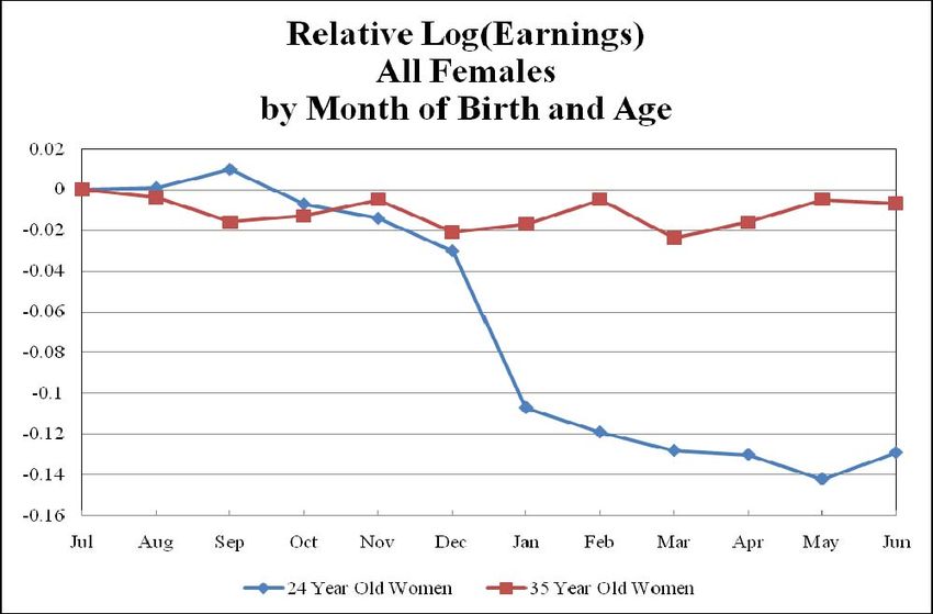
In Figures 5 – 10, we plot the estimates on the month of birth dummies from
regressions that simply regress the outcome variable on the month of birth of the
individual and the year of birth dummies.33 These are essentially descriptions of the
reduced forms underlying our earlier 2SLS estimates. The January effect is normed to
zero in all figures. These figures provide a simple description of the raw data that
provides intuition for the model estimates. It is important to remember that each point in
the figures is an estimate and so much of the variation can be attributed to sampling error.
Even still, the reduced form effects of ESSA underlying our 2SLS estimates are clearly
32
One might still be concerned that 35 is too young an age to cease the analysis. We have information on
ESSA, but not SSA, for cohorts born between 1950 and 1962 and we have used the 1950-1965 cohorts to
estimate the reduced forms all the way from ages 22 to 40. As can be seen in Appendix Figures 2 and 3, the
ESSA effect between 36 and 40 is always close to zero and never statistically significant. Given the
generally high compliance rates, this suggests the SSA effect is also very small for these ages.
33
We do not have an analogous figure for IQ because, given the age-at-test effects, there is no clear
relationship between month of birth coefficients and the estimated SSA coefficient.
30visible for teen pregnancy and for earnings at age 24, as the jump between December and
January is very apparent. On the other hand, the basis for finding no SSA effect on male
education and earnings at age 35 is also obvious, as there is no jump between December
and January for these outcomes.
Heterogeneous Effects of SSA
One concern might be that, by looking at the entire sample, we are missing
important differences across the distribution of children. One might expect the effects of
school starting age to differ based on the family’s characteristics. For example, children
from poorer families may be more at risk and hence suffer most from being young in
school; wealthier families may be able to better offset any negative school effects. On the
other hand, the advantage of school environment over home environment could be
greater for children from poorer backgrounds.
To examine this directly, we regress each outcome (by gender) on a variety of
family background characteristics (mother’s education, family size, and birth order) and
obtain a predicted value for each individual. Using this predicted value as our index of
family background (essentially just a weighted average of the three family background
characteristics), we divide the sample into 4 quartiles and present the results separately
for the first quartile, the second and third quartiles, and the fourth quartile. Table 10
presents these results.
As can be seen, there is little evidence of heterogeneous effects when the outcome
variables considered are IQ, teen pregnancy, or educational attainment. However, the
effect of SSA on the probability of giving birth within 12 years of starting school is
31You can also read