Design Inspiration from Generative Networks
←
→
Page content transcription
If your browser does not render page correctly, please read the page content below
Design Inspiration from Generative Networks
                                                                             ∗
                                                        Othman Sbai1,2, Mohamed Elhoseiny1,∗ Antoine Bordes1
                                                                    Yann LeCun1,3 Camille Couprie1
                                            1 Facebook AI Research, 2 Ecole des ponts, Université Paris Est, 3 New York University

                                                                                         Abstract
arXiv:1804.00921v2 [cs.LG] 14 Sep 2018

                                             Can an algorithm create original and compelling fashion designs to serve as an inspirational assis-
                                             tant? To help answer this question, we design and investigate different image generation models
                                             associated with different loss functions to boost creativity in fashion generation. The dimensions
                                             of our explorations include: (i) different Generative Adversarial Networks architectures that start
                                             from noise vectors to generate fashion items, (ii) novel loss functions that encourage creativity,
                                             inspired from Sharma-Mittal divergence, a generalized mutual information measure for the widely
                                             used relative entropies such as Kullback-Leibler, and (iii) a generation process following the key
                                             elements of fashion design (disentangling shape and texture components). A key challenge of this
                                             study is the evaluation of generated designs and the retrieval of best ones, hence we put together
                                             an evaluation protocol associating automatic metrics and human experimental studies that we hope
                                             will help ease future research. We show that our proposed creativity losses yield better overall ap-
                                             preciation than the one employed in Creative Adversarial Networks. In the end, about 61% of our
                                             images are thought to be created by human designers rather than by a computer while also being
                                             considered original per our human subject experiments, and our proposed loss scores the highest
                                             compared to existing losses in both novelty and likability.

                                         Figure 1: Training generative adversarial models with appropriate losses leads to realistic and cre-
                                         ative 512 × 512 fashion images.

                                         1. Introduction

                                         Artificial Intelligence (AI) research has been making huge progress in the machine’s capability of
                                         human level understanding across the spectrum of perception, reasoning and planning (He et al.,
                                         2017; Andreas et al., 2016; Silver et al., 2016). Another key yet still relatively understudied direc-
                                         tion is creativity where the goal is for machines to generate original items with realistic, aesthetic
                                         and/or thoughtful attributes, usually in artistic contexts. We can indeed imagine AI to serve as in-
                                         spiration for humans in the creative process and also to act as a sort of creative assistant able to help
                                         with more mundane tasks, especially in the digital domain. Previous work has explored writing pop
                                         songs (Briot et al., 2017), imitating the styles of great painters (Gatys et al., 2016; Dumoulin et al.,
                                         2017) or doodling sketches (Ha and Eck, 2018) for instance. However, it is not clear how creative
                                         such attempts can be considered since most of them mainly tend to mimic training samples without

                                                                                              1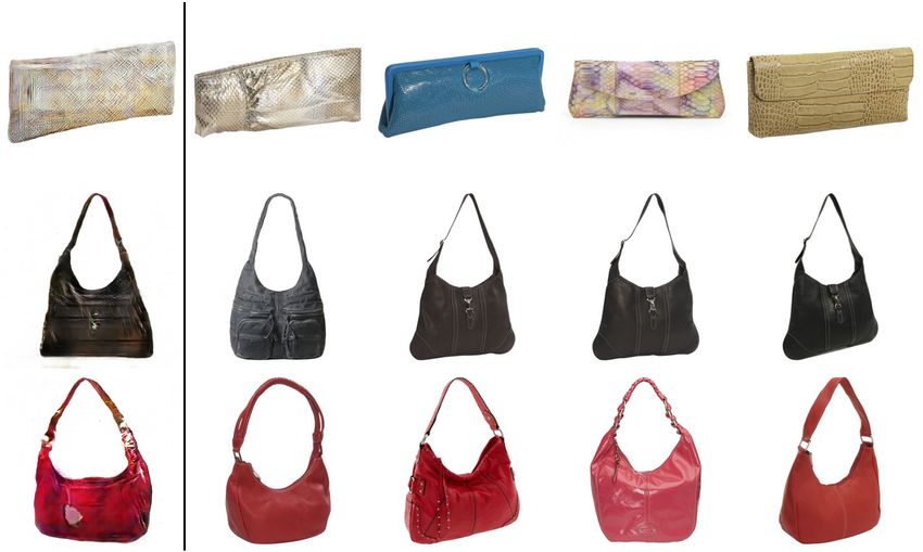
expressing much originality. Creativity is a subjective notion that is hard to define and evaluate, and
even harder for an artificial system to optimize for. Colin Martindale put down a psychology based
theory that explains human creativity in art (Martindale, 1990) by connecting creativity or accept-
ability of an art piece to novelty with “the principle of least effort”. As originality increases, people
like the work more and more until it becomes too novel and too far from standards to be understood.
When this happens, people do not find the work appealing anymore because a lack of understand-
ing and of realism leads to a lack of appreciation. This behavior can be illustrated by the Wundt
curve that correlates the arousal potential (i.e. novelty) to hedonic responses (e.g. likability of the
work) with an inverted U-shape curve. Earlier works on computational creativity for generating
paintings have been using genetic algorithms (Machado et al., 2008; Machado and Cardoso, 2000;
Mordvintsev et al., 2015) to create new artworks by starting from existing human-generated ones
and gradually altering them using pixel transformation functions. There, the creativity is guided by
pre-defined fitness functions that can be tuned to trade-off novelty and realism. For instance, for
generating portraits, DiPaola and Gabora (2009) define a family of fitness functions based on spe-
cific painterly rules for portraits that can guide creation from emphasizing resemblance to existing
paintings to promoting abstract forms.

Generative Adversarial Networks (GANs) (Goodfellow et al., 2014; Radford et al., 2016) show a
great capability to generate realistic images from scratch without requiring any existing sample to
start the generation from. They can be applied to generate artistic content, but their intrinsic creativ-
ity is limited because of their training process that encourages the generation of items close to the
training data distribution; hence they show limited originality and overall creativity. Similar conser-
vative behavior can be seen in recent deep learning models for music generation where the systems
are also mostly trained to reproduce pattern from training samples, like Bach chorales (Hadjeres
and Pachet, 2017). Creative Adversarial Networks (CANs, Elgammal et al. (2017)) have then been
proposed to adapt GANs to generate creative content (paintings) by encouraging the model to de-
viate from existing painting styles. Technically, CAN is a Deep Convolutional GAN (DCGAN)
model (Radford et al., 2016) associated with an entropy loss that encourages novelty against known
art styles. The specific application domain of CANs allows for very abstract generations to be ac-
ceptable but, as a result, does reward originality a lot without judging much how such enhanced
creativity can be mixed with realism and standards.

In this paper we study how AI can generate creative samples for fashion. Fashion is an interesting
domain because designing original garments requires a lot of creativity but with the constraints that
items must be wearable. For decades, fashion designers have been inventing styles and innovating
on shapes and textures while respecting clothing standards (dimensions, etc.) making fashion a
great playground for testing AI creative agents while also having the potential to impact everyday
life. In contrast to most generative models works, the creativity angle we introduce makes us go
beyond replicating images seen during training. Fashion image generation opens the door for break-
ing creativity into design elements (shape and texture in our case), which is a novel aspect of our
work in contrast to CANs. More specifically, this work explores various architectures and losses
that encourage GANs to deviate from existing fashion styles covered in the training dataset, while
still generating realistic pieces of clothing without needing any image as input. In the fashion indus-
try, the design process is traditionally organized around the collaboration between pattern makers,
responsible for the material, the fabric and the texture, and sample makers, working on the shape
models. As detailed in Table 1, we follow a similar process in our exploration of losses and architec-

                                                   2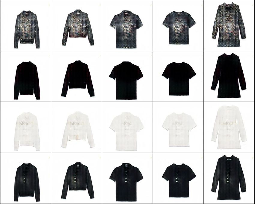
Architecture                      Creativity Loss              Design Elements
       DCGAN (Radford et al., 2016)     CAN (Elgammal et al., 2017)          Texture (ours)
           StackGAN (ours)                      MCE (ours)                    Shape (ours)
           StyleGAN (ours)             Bhattacharyya divergence (ours)   Shape & Texture (ours)

Table 1: Dimensions of our study. We propose fashion image generation models that differ in their
architecture and their creativity loss that encourages the generations to deviate from existing shapes,
textures, or both.

tures. We compare the relative impact of both shape and texture dimensions on final designs using
a comprehensive evaluation that jointly assesses novelty, likeness and realism using both adapted
automatic metrics, and extensive humans subject experiments. To the best of our knowledge, this
work is the first attempt at incorporating creative fashion generation by explicitly relating it to its
design elements. Our contributions are the following:
   • We are the first to propose a creativity loss on image generation of fashion items with a
     specific conditioning of texture and shape, learning a deviation from existing ones.
   • We are the first to propose the better leading results, more general, multi-class cross entropy
     criterion for learning to deviate from existing shapes and textures. We also express it as a
     particular occurrence of the Sharma-Mittal divergence as a generalized entropy that promotes
     generating creative fashion products, allowing the exploration of various settings.
   • We re-purpose automatic entropy based evaluation criteria for assessment of fashion items in
     terms of texture and shape; The correlations between the automatic metrics that we proposed
     and our human study allow us to draw some conclusions with useful metrics revealing human
     judgment.
   • We propose a concrete solution to make our Style GAN model conditioned on shape images
     work in a non-deterministic way, and trained it with creative losses, resulting in a novel and
     powerful model.
As illustrated in Fig. 1, our best models manage to generate realistic images with high resolution
512 × 512 using a relatively small dataset (about 4000 images). More than 60% of our generated
designs are judged as being created by a human designer while also being considered original, show-
ing that an AI could offer benefits serving as an efficient and inspirational assistant. A preliminary
version of this work appears in (Sbai et al., 2018) and is significantly extended here.

2. Related work

There has been a growing interest in generating images using convolutional neural networks and
adversarial training, given their ability to generate appealing images unconditionally, or condition-
ally like from text, class labels, and for paired and unpaired image translations (Zhu et al., 2017a).
GANs (Goodfellow et al., 2014) allow image generation from random numbers using two networks
trained simultaneously: a generator is trained to fool an adversarial network by generating images
of increasing realism. The initial resolution of generated images was 32 × 32. From this seminal
work, progresses were achieved in generating higher resolution images, using a cascade of convolu-
tional networks (Denton et al., 2015) and deeper network architectures (Radford et al., 2016). The

                                                  3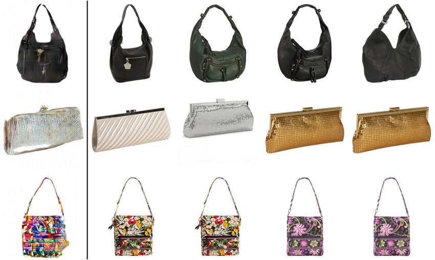
introduced of auxiliary classifier GANs (Odena et al., 2017) then consisted to add a label input in
addition to the noise and training the discriminator to classify the synthesized 128 × 128 images.
The addition of text inputs (Reed et al., 2016; Zhang et al., 2017) allowed the generative network
to focus on the area of semantic interest and generate photo-realistic 256 × 256 images. Recently,
impressive 1024 × 1024 results were obtained using a progressive growing of the generator and
discriminator networks (Karras et al., 2018), by training models during several tens of days.
Neural style transfer methods (Gatys et al., 2016; Johnson et al., 2016) opened the door to the
application of existing styles on clothes (Date et al., 2017), the difference with generative models
being the constraint to start from an existing image in input. Isola et al. (2017) relax this constraint
partly by starting from a binary image of edges, and present some generation of handbags images.
Another way to control the appearance of the result is to enforce some similarity between input
texture patch and the resulting image (Xian et al., 2018). Using semantic segmentation and large
datasets of people wearing clothes, (Zhu et al., 2017b; Lassner et al., 2017) generate full bodies
images and are conditioning their outputs either on text descriptions, color or pose information. In
this work, we are interested in exploring the creativity of generative models and focus on presenting
results using only random or shape masks as inputs to leave freedom for a full exploration of GANs
creative power.

3. Models: architectures and losses

Table 1 summarizes our models and losses exploration. Let us consider a dataset D of N images. Let
xi be a real image sample and zi a vector of n of real numbers sampled from a normal distribution.
In practice n = 100.

3.1 GANs

As in (Goodfellow et al., 2014; Radford et al., 2016), the generator parameters θG are learned to
compute examples classified as real by D:
                                                X
                        min LG real/fake = min       log(1 − D(G(zi ))).
                           θG                   θG
                                                     zi ∈Rn

The discriminator D, with parameters θD , is trained to classify the true samples as 1 and the gener-
ated ones as 0:

                                            X
               min LD real/fake = min                   − log D(xi ) − log(1 − D(G(zi ))).
                θD                 θD
                                        xi ∈D, zi ∈Rn

3.2 GANs with classification loss

Following (Odena et al., 2017), we use shape and texture labels to learn a shape classifier and a
texture classifier in the discriminator. Adding these labels improves over the plain model and stabi-
lizes the training for larger resolution. Let us define the texture and shape integer labels of an image

                                                        4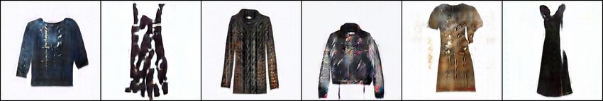
sample x by t̂ and ŝ respectively. We are adding to the discriminator network either one branch
for texture Dt or shape Ds classification or two branches for both shape and texture classification
D{t,s} . In the following section, for genericity, we employ the notation Db,k , designating the output
of the classification branch b for class k ∈ {1, ..., K}, where K is the number of different possible
classes of the considered branch (shape or texture). We add to the discriminator loss the following
classification loss:
                                                                                                             !
                                                                     X                  eDb,ĉi (xi )
      LD = λDr LD real/fake + λDb LDclassif with LD classif = −              log       PK                        ,
                                                                                                Db,k (xi )
                                                                     xi ∈D              k=1 e

where cˆi is the label of the image xi for branch b.

3.3 Creativity losses

Because GANs learn to generate images very similar to the training images, we explore ways to
make them deviate from this replication by studying the impact of an additional loss for the gener-
ator. The final loss of the generator that is optimized jointly with LD is:

                                  LG = λGr LG real/fake + λGe LG creativity

We explored different losses for creativity that we detail in this section. First, we employ binary
cross entropies over the adversarial network outputs as in CANs. Second, we suggest to employ the
multi-class cross entropy (MCE) as a natural way to normalize the penalization across all classes.
Finally, we show that this MCE loss is equivalent to a KL entropy and further generalize the cre-
ativity expression to the family of Sharma-Mittal divergences (Akturk et al., 2007).

Binary cross entropy loss (CAN (Elgammal et al., 2017)). Given the adversarial network’s
branch Dc trained to classify different textures or shapes, we can use the CAN loss LCAN as
LG creativity to create a new style that confuses Db :

                      K
                     XX 1                         K −1
         LCAN = −         log(σ(Db,k (G(zi )))) +      log(1 − σ(Db,k (G(zi )))),                                    (1)
                        K                          K
                        i   k=1

where σ denotes the sigmoid function.

Multi-class Cross Entropy loss. We propose to use as LG creativity the Multi-class Cross Entropy
(MCE) loss between the class prediction of the discriminator and the uniform distribution. The goal
is for the generator to make the generations hard to classify by the discriminator.
                              K                                           K
                                                                !
                         XX       1          eDb,k (G(zi ))          XX       1
             LMCE = −               log PK                        =−            log(D̂i ),      (2)
                                 K          q=1 e
                                                  Db,q (G(zi ))              K
                            i   k=1                                          i   k=1

where D̂i is the softmax of Db (G(zi )). In contrast to the CAN loss that treats every classification
independently, the MCE loss should better exploit the class information in a global way.

                                                     5
Our MCE loss is in fact equivalent to a Kullback-Leibler (KL) loss between a uniform distribution
and the softmax output, since the entropy term of the uniform distribution is constant; see derivation
in Eq. 3.

         X 1         1       X 1       1    X 1                 X 1
 LKL =         log(       )=       log( ) −       log(D̂i ) ∝ −       log(D̂i ) = LMCE (3)
             K      K D̂i        K     K        K                   K
         i,k                 i,k            i,k                 i,k

It is more meaningful conceptually to define the deviation over the joint distribution over the cate-
gories which is what we modeled by the KL divergences between the softmax probabilities and the
prior (defined as uniform in our case), as it also opens the door to study other divergence measures.
Finally, the MCE loss requires less compute comparing to CAN.

Figure 2: Some generations from a DCGAN with MCE creativity loss applied on texture (Model
GAN MCE tex).

Generalized Sharma-Mittal Divergence. We further generalize the expression of the creativity
term to a broader family of divergences, unlocking new way of enforcing deviation from existing
shapes and textures. Akturk et al. (2007) studied an entropy measure called Sharma-Mittal which
was originally introduced by Sharma (1975). Given two parameters (α and β), the Sharma-Mittal
(SM) divergence SMα,β (pkq), between two distributions p and q is defined ∀α > 0, α 6= 1, β 6= 1
as                                                "                          #
                                              1     X                1−β
                       SM (α, β)(p||q) =               (pi1−α qi α ) 1−α − 1                  (4)
                                            β−1
                                                        i
It was shown in (Akturk et al., 2007) that most of the widely used divergence measures are spe-
cial cases of SM divergence. For instance, each of the Rényi, Tsallis and Kullback-Leibler (KL)
divergences can be defined as limiting cases of SM divergence as follows:
                                                    1      X
                                                                    1−α
                       Rα (pkq) = lim SMα,β (pkq) =     ln(     pα
                                                                 i qi   )),
                                β→1                α−1       i
                                                    1 X α 1−α
                      Tα (pkq) = lim SMα,β (pkq) =      (     p q     ) − 1),                      (5)
                                β→α                α−1 i i i
                                                      X          pi
                      KL(pkq) = lim SMα,β (pkq) =         pi ln( ).
                                β→1,α→1
                                                       i
                                                                 qi

In particular, the Bhattacharyya divergence (Kailath, 1967), denoted by B(pkq) is a limit case of
SM and Rényi divergences as follows as β → 1, α → 0.5
                                                                    X
                      B(pkq) = 2      lim      SMα,β (pkq) = − ln        p0.5
                                                                          i qi
                                                                              0.5
                                                                                    .
                                   β→1,α→0.5
                                                                     i

                                                    6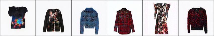
Since the notion of creativity in our work is grounded to maximizing the deviation from existing
shapes and textures through KL divergence in Eq 3, we can generalize our MCE creativity loss by
minimizing Sharma Mittal (SM) divergence between a uniform distribution and the softmax output
D̂ as follows

                                                             1 X 1 1−α α 1−α1−β
        LSM = SM (α, β)(D̂||u) = SM (α, β)(D̂||u) =             (     D̂i )     −1                (6)
                                                            β−1   K
                                                                     i

Note that the MCE loss in Eq 3 is a special case of the generalized SM loss where α → 1 and
β → 1 (i.e., KL divergence). Similarly, Tsallis , and Renyi, and Bhattacharyya losses are special
cases of SM loss where α = β, β → 1 and α → 0.5 and β → 1. We explored various parameters
but we found both KL and Bhattacharyya losses work the best and hence we focus on them in our
experiments. We denote models trained with these losses by MCE and SM respectively.

3.4 Network architectures

We experiment using three architectures : modified versions of the DCGAN model (Radford et al.,
2016), StackGANs (Zhang et al., 2017) with no text conditioning, and our proposed styleGAN.

DCGAN. The DCGAN generator’s architecture was only modified to output 256×256 or 512×512
images. The discriminator architecture also includes these modifications and contains additional
classification branches depending on the employed loss function.

Unconditional StackGAN. Conditional StackGAN (Zhang et al., 2017) has been proposed to gen-
erate 256×256 images conditioned on captions. The method first generates a low resolution 64×64
image conditioned on text. Then, the generated image and the text are tiled on a 16 × 16 × 512
feature map extracted from the 64 × 64 generated image to compute the final 256 × 256 image.
We adapted the architecture by removing the conditional units (i.e. the text) but realized that it did
not perform well for our application. The upsampling in (Zhang et al., 2017) was based on nearest
neighbors which we found ineffective in our setting. Instead, we first generate a low resolution
image from normal noise using a DCGAN architecture (Radford et al., 2016), then conditioning on
it, we build a higher resolution image of 256 × 256 with a generator inspired from the pix2pix archi-
tecture with 4 residual blocks (Isola et al., 2017). The upsampling was performed using transposed
convolutions. The details of the architecture are provided in the appendix.

StyleGAN: Conditioning on masks. To grant more control on the design of new items and get
closer to standard fashion processes where shape and texture are handled by different specialists, we
also introduce a model taking binary masks representing a desired shape in input. Since that even
for images on white background a simple threshold fails to extract accurate masks, we compute
them using the graph based random walker algorithm (Grady, 2006).
In the StyleGAN model, a generator is trained to compute realistic images from a mask input and
noise representing style information (see Fig. 3), while a discriminator is trained to differentiate
real from fake images. We use the same discriminator architecture as in DCGAN with classifier
branches that learn shape and texture classification on the real images on top of predicting real/fake
discrimination.

                                                  7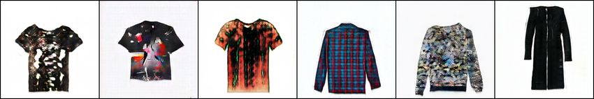
Figure 3: From the segmented mask of a fashion item and different random vector z, our StyleGAN
model generates different styled images.

Previous approaches of image to image translation such as pix2pix (Isola et al., 2017) and Cy-
cleGAN (Zhu et al., 2017a) create a deterministic mapping between an input image to a single
corresponding one, i.e. edges to handbags for example or from one domain to another. This is due
to the difficulty of training a generator with two different inputs, namely mask and style noise, and
making sure that no input is being neglected. In order to allow sampling different textures for the
same shape as a design need, we avoid this deterministic mapping by enforcing an additional `1 loss
on the generator:

                                      XX
                             Lrec =              |G(mi,p , zi = 0) − mi,p |,                       (7)
                                       i   p∈P

where mi,p denotes the mask of a sample image xi at pixel p, and P denotes the set of pixels of
mi . This loss encourages the reconstruction of the input mask in case of null input z (i.e. zeros) and
hence ensures the disentanglement of the shape and texture: having the reconstruction of the shape
for null vector z encourages the z to only capture the texture variation. The architecture is detailed
in the appendix.

4. Experiments

After presenting our datasets, we describe some automatic metrics we found useful to sort models
in a first assessment, present quantitative results followed by our human experiments that allow us
to identify the best models.

4.1 Datasets

Unlike similar work focusing on fashion item generation (Lassner et al., 2017; Zhu et al., 2017b),
we choose datasets which contain fashion items in uniform background allowing the trained models
to learn features useful for creative generation without generating wearers face and the background.
We augment each dataset 5 times by jittering images with random scaling and translations.

                                                     8
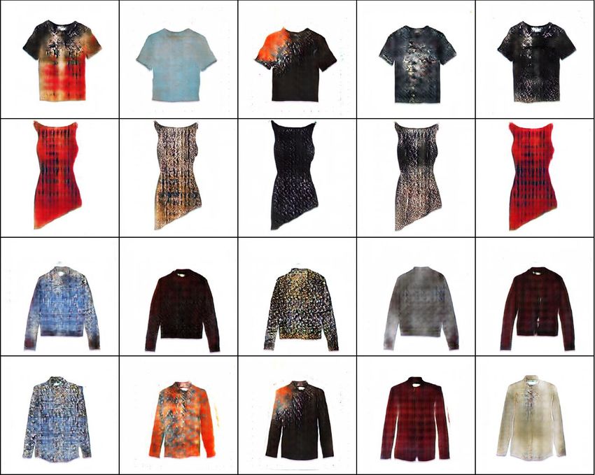
Figure 4: From the mask of a product, our StyleGAN model generates different styled image for
each style noise.

The RTW dataset. We have at our disposal a set of 4157 images of different Ready To Wear
(RTW) items of size 3000 × 3760. Each piece is displayed on uniform white background. These
images are classified into seven clothes categories: jackets, coats, shirts, tops, t-shirts, dresses and
pullovers, and 7 texture categories: uniform, tiled, striped, animal skin, dotted, print and graphical
patterns.

Attribute discovery dataset. We extracted from the Attribute discovery dataset (Berg et al., 2010)
5783 images of bags, keeping for our training only images with white background. There are seven
different handbags categories: shoulder, tote, clutch, backpack, satchel, wristlet, hobo. We also
classify these images by texture into the same 7 texture classes as the RTW dataset.

4.2 Automatic evaluation metrics

Training generative models on fashion datasets generates impressive designs mixed with less im-
pressive ones, requiring some effort of visual cherry-picking. We propose some automated criteria to
evaluate trained models and compare different architectures and loss setups. We study in Section 4.4
how these automatic metrics correlate with the human evaluation of generated images.
Evaluating the diversity and quality of a set of images has been tackled by scores such as the in-
ception score and variants like the AM score (Zhou et al., 2017). We adapt both of them for our
two attributes specific to fashion design (shape and texture) and supplement them by a mean nearest
neighbor distance. Our final set of automatic scores contains 10 metrics:
   • Shape score and texture score, each based on a Resnet-18 classifier of (shape or texture re-
     spectively);
   • Shape AM score and texture AM score, based on the output of the same classifiers;
   • Distance to nearest neighbors images from the training set;
   • Texture and shape confusion of classifier;
   • Darkness, average intensity and skewness of images;

                                                   9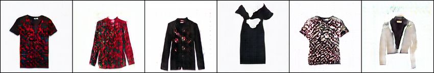
Inception-like scores. The Inception score (Salimans et al., 2016; Warde-Farley and Bengio, 2017)
was introduced as a metric to evaluate the diversity and quality of generations, with respect to the
output of a considered classifier (Szegedy et al., 2017). For evaluating N samples {x}N     1 , it is
computed as
                         Iscore ({x}N
                                    1 ) = exp(E[KL(c(x)||E[c(x)])])),

where c(x) is the softmax output of the trained classifier c, originally the Inception network.

Intuitively, the score increases with the confidence in the classifier prediction (low entropy score) of
each image and with the diversity of all images (high overall classification entropy). In this paper,
we exploit the shape and texture class information from our two datasets to train two classifiers on
top of Resnet-18 (He et al., 2015) features, leading to the shape score and texture score.

AM scores. We also use the AM score proposed in (Zhou et al., 2017). It improves over the
inception score by taking into consideration the distribution of the training samples x̄ as seen by the
classifier c, which we denote c̄train = E[c(x̄)]. The AM score is calculated as follows:

                  AMscore ({x}N
                              1 ) = E[KL(c̄
                                           train
                                                 ||c(x)] − KL(c̄train ||E[c(x)])]

The first term is maximized when each of the generated samples is far away from the overall training
distribution, while the second term is minimized when the overall distribution of the generations is
close to that of the training. In accordance with (Zhou et al., 2017), we find that this score is more
sensible as it accounts for the training class distribution.

Nearest neighbors distance. To be able to assess the creativity of the different models while
making sure that they are not reproducing training samples, we compute the mean distance for each
sample to its retrieved k-Nearest Neighbors (NN), with k = 10, as the Euclidean distance between
the features extracted from a Resnet18 pre-trained on ImageNet(He et al., 2015) by removing its last
fully connected layer. These features are of size 512. This score gives an indicator of the similarity
to the training data. A high NN distance may either mean that the generated images has some
artifacts, in this case, it could be seen as an indicator of failure, or it could mean that the generation
is novel and highly creative.

Figure 5: First column: random generations by the GAN MCE shape model. Four left columns:
Retrieved Nearest Neighbors for each sample.

                                                   10
Darkness and Average intensity. Dark colors might be preferred for fashion items as they are
perceived as fitting well with other colors. From the Y component of an image of a Y U V decom-
position, this score counts the number of pixels whose brightness Y is below a threshold (0.35). The
average intensity score is also computed from the Y component.
Skewness. The third order moment of the image histogram has been shown to be informative about
image aesthetic (Motoyoshi et al., 2007; Attewell and Baddeley, 2007). It computes the asymmetry
of color intensity distribution. We chose to compute it from the histogram of the Y channel of a
Y U V decomposition.
Shapes and texture confusion scores. Given an image x, we may compute a score that reflects
the confusion of the shape or texture classifier
K
!
X eci (x) eci (x)
Cscore (x) = − P c (x) ln P c (x) , (8)
ke ke
k k
i=1
where ck (x) denotes the output of classifier c. This score is high when the texture or shape of the
image is easy to identify.
Shapes and texture categories.
It might be useful to determine if the generation of particular categories of clothes (shapes or tex-
tures) plays a role into the likeliness of images. We therefore apply our shape and texture classifier
to generated images.
4.3 Automatic evaluation results
We experiment using weights λGe of 1 and 5 for the MCE creativity loss. It appeared that the weight
1 worked better for the bags dataset, and 5 for the RTW dataset. We also tried different weights
for the CAN and SM loss but they did not have a large influence on the results and was fixed to
1. All models were trained using the default learning rate 0.002 as in (Radford et al., 2016). Our
different models take about half a day to train on 4 Nvidia P100 GPUs for 256 × 256 models and
almost 2 days for the 512 × 512 ones. In our study, it was more convenient from a memory and
computational resources standpoint to work with 256 × 256 images but we also provide 512 × 512
results in Fig. 1 to demonstrate the capabilities of our approach. For each setup, we manually select
four saved models after a sufficient number of iterations. Our models produce plausible results after
training for 15000 iterations with a batch size of 64 images.
Table 2 presents shape and texture classifier confidence C scores, AM scores (for shape and texture),
average NN distances computed for each model, Average intensity and Darkness scores on a set
of 100 randomly selected images. Our first observation is that the DCGAN model alone seems
to perform worse than all other tested models with the highest NN distance and lower shape and
texture scores. The value of the NN distance score may have different meanings. A high value could
mean an enhanced creativity of the model, but also a higher failure rate.
For the RTW dataset, the two models having high AM texture score, and high NN distances scores
are DCGAN with MCE loss models and Style CAN with texture creativity. On the handbags
11C sh AM sh C tex AM tex NN Average Dark
GAN 0.26 7.88 0.39 2.07 14.2 194 5719
GAN classif 0.27 9.78 0.58 1.58 13.0 188 7324
GAN MCE sh 0.31 8.22 0.59 1.69 13.1 192 6667
GAN MCE tex 0.25 8.05 0.59 2.33 13.8 194 5617
GAN MCE shTex 0.21 8.96 0.49 1.45 13.3 190 5843
CAN sh 0.27 8.52 0.48 1.86 13.2 192 6524
CAN tex 0.29 8.40 0.48 2.24 13.4 190 6103
CAN shTex 0.19 10.1 0.46 2.39 13.2 192 6958
SM tex 0.23 9.89 0.43 2.44 12.9 193 7112
SM sh 0.19 9.39 0.51 1.21 12.3 191 8663
SM shtex 0.22 8.86 0.51 1.75 14.1 198 6738
StackGAN 0.25 8.82 0.52 1.95 12.9 193 7735
StackGAN MCE sh 0.27 8.16 0.64 2.03 13.6 195 6098
StackGAN MCE tex 0.26 8.55 0.63 1.68 13.2 186 8483
StackGAN MCE shTex 0.27 7.90 0.71 1.91 13.6 194 4921
StackCAN sh 0.20 8.96 0.67 1.46 12.7 189 9019
StackCAN tex 0.22 9.45 0.49 2.32 13.2 189 8796
StackCAN shTex 0.26 8.11 0.67 2.07 13.4 193 5737
style GAN 0.25 8.24 0.52 1.76 13.7 198 6622
style CAN tex 0.29 7.93 0.48 2.05 13.9 193 6904
style GAN MCE tex 0.34 7.35 0.49 1.49 13.4 190 9570
(a) Ready To Wear dataset
C sh AM sh C tex AM tex NN Average Dark
GAN 0.43 3.65 1.71 1.57 20.8 205 2234
CAN tex 0.35 4.29 1.79 1.60 21.4 201 1615
CAN sh 0.39 4.23 1.88 1.26 21.0 201 2617
CAN sh tex 0.39 3.93 1.89 1.56 21.1 203 1954
GAN MCE tex 0.34 4.38 1.99 1.60 21.6 196 2691
GAN MCE sh 0.38 4.15 1.98 1.84 20.8 207 1593
GAN MCE sh tex 0.42 3.73 2.00 1.80 21.0 200 2333
(b) Attribute bags dataset
Table 2: Quantitative evaluation on the RTW dataset and bag datasets. For better readability we
only display metrics that correlate most with human judgment. Higher scores, highlighted in bold,
are usually preferred.
datasets, the models obtaining the best metrics overall are the DCGAN with MCE creativity losses
texture alone or on shape and texture. To show that our models are not reproducing exactly samples
from the dataset, we display in Fig. 5 results from the model having the lowest NN distance score,
with its 4 nearest neighbors. We note that even if uniform bags tend to be similar to training data,
complex prints show high differences. These differences are amplified on the RTW dataset.
Creating evaluation sets.
Motivated by the will of accessing automatically the best generations from each model, we extract
different clusters of images with particular visual properties that we want to associate with realism,
overall appreciation and creativity. Given the selected models, 10000 images are generated from
12random numbers – or randomly selected masks for the styleGAN model – to produce 8 sets of 100
images each. Based on the shape entropy, texture entropy and mean nearest neighbors distance of
each image we can rank the generations and select the ones with (i) high/low shape entropy, (ii)
high/low texture entropy, (iii) high/low NN distance to real images. We also explore random and
mixed sets such as low shape entropy and high nearest neighbors distance. We expect such a set to
contain plausible generations since low shape entropy usually correlates with well defined shapes,
while high nearest neighbor distance contains unusual designs. Overall, we have 8 different sets
that may overlap. We choose to evaluate 100 images for each set.
4.4 Human evaluation results
Figure 6: Best generations of handbags as rated by human annotators. Each question is in a row.
Q1: overall score, Q2: shape novelty.
We perform a human study where we evaluate different sets of generations of interest on a designed
set of questions in order to explore the correlations with each of the proposed automatic metrics in
choosing best models and ranking sound generations. As our RTW garment dataset could not be
made publicly available, we conducted two independent studies:
1. In our main human evaluation study, 800 images - selected as described in the previous section
- per model were evaluated, each image evaluated by 5 different persons. There were in average
90 participants per model assessment, resulting in average to 45 images assessed per participant.
Since the assessment was conducted given the same conditions for all models, we are confident
that the comparative study is fair. Each subject is shown images from the 8 selected sets described
in the previous section and is asked 6 questions:
• Q1: how do you like this design overall on a scale from 1 to 5?
• Q2/Q3: rate the novelty of shape (Q2) and texture (Q3) from 1 to 5.
• Q4/Q5: rate the complexity of shape (Q4) and texture (Q5) from 1 to 5.
• Q6: Do you think this image was created by a fashion designer or generated by computer?
(yes/no)
Each image is annotated by taking the average rating of 5 annotators.
132. We conducted another study in our lab were we mixed both generations (500 total images picked
randomly from 5 best models) and 300 real down-sampled images from the RTW dataset. We
asked if the images were real or generated to about 45 participants who rated 20 images each in
average. We obtain 20% of the generations thought to be real, and 21.5% of the original dataset
images were considered to be generated.
Likeability
Method/Human over- shape shape tex. tex. real
Method all nov. comp. nov. comp. fake
DCGAN MCE shape 3.78 3.58 3.57 3.64 3.57 60.9
76 GAN MCE sh DCGAN MCE tex 3.72 3.57 3.52 3.61 3.58 61.1
GAN MCE tx StyleCAN tex 3.65 3.37 3.31 3.44 3.21 49.7
StackGAN 3.62 3.45 3.38 3.43 3.33 51.9
74 StyleCAN tx
StyleGAN MCE tex 3.61 3.38 3.29 3.50 3.37 53.4
StyleGAN MCE tx DCGAN SM tx 3.60 3.43 3.42 3.46 3.41 52.6
72 SM tex StackGAN MCE tex 3.59 3.36 3.31 3.44 3.28 55.9
StyleGAN 3.59 3.28 3.21 3.27 3.15 47.2
GAN MCE shTex StackGAN CAN sh 3.51 3.56 3.56 3.58 3.40 50.7
70 DCGAN MCE shTex 3.49 3.40 3.24 3.40 3.31 61.3
GAN classif CAN sh tx StackGAN CAN tex 3.48 3.57 3.54 3.55 3.50 48.4
SM sh DCGAN CAN shTex 3.47 3.28 3.18 3.33 3.16 63.8
68 CAN tx
StackGAN MCE sh 3.45 3.27 3.16 3.28 3.12 60.4
CAN sh
StackGAN CAN shTex 3.42 3.37 3.32 3.44 3.32 49.5
66 DCGAN classif 3.42 3.32 3.32 3.37 3.29 52.7
GAN DCGAN SM sh 3.39 3.27 3.12 3.30 3.23 55.1
SM sh tex DCGAN CAN tex 3.37 3.23 3.12 3.35 3.09 59.7
64 DCGAN CAN sh 3.33 3.28 3.16 3.27 3.12 55.0
StackGAN MCE shtex 3.30 3.25 3.28 3.31 3.27 41.5
45 50 55 60 65 DCGAN 3.22 2.95 2.78 3.24 2.83 60.4
DCGAN SM shTex 3.20 3.10 3.00 3.13 3.1 45.5
Real appearance
Figure 7: Human evaluation on the 800 images from all sets ranked by decreasing overall score
(higher is better) on the RTW dataset. Evaluation of the different models on the RTW dataset
by human annotators on two axis: likability and real appearance. Our models using MCE, SM
creativity or shape conditioning are highlighted by darker colors. They reach nice trade-offs between
real appearance and likability.
Table 7 presents the average scores obtained by each model on each human evaluation question for
the RTW dataset. From this table, we can see that using our creativity loss (MCE shape and MCE
tex) performs better than the DCGAN baseline. We obtain a similar ranking of the models on the set
of random images. The image set of ’low NN distance’ contains the most popular images, with an
average of 4.16 overall score for the best model. We checked the statistical significance of the results
of Table 7 by computing paired Student t-tests. The obtained p-value between the overall scores of
the two first ranked models is 0.03, and the one between the first and the third ranked models is
lower than 10−6 , allowing us to reject the hypothesis of statistically equal averages.
Fig. 7 shows how well our approaches worked on two axis: likability and real appearance. The most
popular methods are obtained by the models employing creativity loss and in particular our proposed
MCE loss, as they are perceived as the most likely to be generated by designers, and the most liked
overall. We are greatly improving the state-of-the-art here, going from a score of 64% to more than
75% in likabity from classical GANs to our best model with shape creativity. Our proposed Style
GAN and StackGAN models are producing competitive scores compared to the best DCGAN setups
with high overall scores. In particular, our proposed StyleGAN model with creativity loss is ranked
14in the top-3, some results are presented in Fig. 4. We display images which obtained the best scores
for each of the 6 questions in Fig. 9, and some results of handbags generation in Fig. 6.
We may also recover the famous Wundt curve mentioned in the introduction by plotting the likability
as a function of the novelty in Fig. 8. The novelty was difficult to assess by raters solely from gen-
erated images, therefore in this diagram, we give the novelty as the average distance from training
images (NN metric). We note that the GAN with classification loss and models with Sharma-Mittal
creativity exhibit low novelty. The most novel model is the classical GAN, however this kind of
novelty is not very much appreciated by the raters. At the top of the curve, most of our new models
based on the MCE or SM loss manage to find a nice compromise between novelty and hedonic
value.
Figure 8: Empirical approximation of the Wundt curve, drawing a relationship between novelty
and appreciation. Models employing our proposed MCE losses appear in red, reaching a good
compromise between novelty and likability.
Human over- shape shape tex. tex. real Human over- shape shape tex. tex. real
Auto all nov. comp. nov. comp. fake Auto all nov. comp. nov. comp. fake
coat 0.14 0.37 0.43 0.21 0.34 0.27
I sh score 0.43 0.65 0.67 0.33 0.60 0.30 top -0.15 0.12 0.16 0.18 0.07 -0.08
AM sh score 0.46 0.66 0.68 0.38 0.64 0.28 shirt 0.43 0.46 0.37 0.07 0.30 0.21
jacket 0.27 0.36 0.31 0.08 0.28 -0.02
C sh score 0.48 0.51 0.55 0.34 0.50 -0.06 t-shirt 0.44 0.49 0.43 0.31 0.49 0.08
I tex score 0.48 0.63 0.62 0.30 0.55 0.28 dress 0.40 0.49 0.57 0.36 0.53 0.12
AM score 0.37 0.47 0.46 0.16 0.42 0.22 pullover 0.24 0.41 0.50 0.32 0.47 0.33
dotted 0.41 0.35 0.40 0.26 0.32 0.25
C tex score 0.48 0.67 0.71 0.48 0.64 0.27 striped 0.20 0.16 0.15 0.08 0.21 0.11
N10 0.46 0.63 0.65 0.33 0.58 0.23 print 0.42 0.31 0.26 0.30 0.35 -0.04
Av. intensity 0.48 0.65 0.66 0.35 0.59 0.23 uniform 0.31 0.51 0.54 0.26 0.51 0.13
tiled 0.23 0.17 0.14 -0.08 -0.01 0.22
Skewness 0.32 0.62 0.66 0.32 0.65 0.31 skin -0.03 0.32 0.32 0.30 0.17 0.17
Darkness 0.28 0.54 0.62 0.32 0.60 0.43 graphical 0.34 0.46 0.47 0.17 0.46 0.20
Table 3: Correlation scores between human evaluation ratings and automatic scores on the set of
randomly sampled images of all models.
Correlations between human evaluation and automatic scores.
From Table 3, we see that the automatic metrics that correlate the most with the overall likability
are the classifiers confidence scores, the inception texture score, and the average intensity. The
15Figure 9: Best generations of RTW items as rated by human annotators. Each question is in a row.
Left: Q1: overall score, Q2: shape novelty, Q3: shape complexity, Right: Q4: texture novelty, Q5:
texture complexity, Q6: Realism.
PCA on metrics on the 'random' set PCA on metrics on the 'low shape entropy' set PCA on metrics on the 'low shape entr. high NN dist.' set
40 low overall score (Q1) 40
medium overall score (Q1) 30
high overall score (Q1) 30
20
20 20
10 10
0 0 0
10 10
20
20 low overall score (Q1) low overall score (Q1)
20
30 medium overall score (Q1) medium overall score (Q1)
40 high overall score (Q1) high overall score (Q1)
30
5000 0 5000 10000 15000 5000 0 5000 10000 15000 5000 0 5000 10000 15000
Figure 10: PCA on image-wise automatic metrics (C tex, C shape, NN dist, Average intensity,
Skewness, Darkness). Each metric was subtracted its mean value. The variables of the two first
components are the Darkness and the Average intensity.
skewness measures correlates well with shape and texture complexity. The best correlated measure
with real appearance is the Darkness as one could expect. Figure 10 complements our analysis on
correlations by presenting projections of the automatic metrics on generations from 3 sets (random,
low shape entropy and low shape entropy and high NN distance). Each data point corresponding
to one image is colored by a function of the human overall rating. The PCA reveals that the two
principal components are mostly explained by the Darkness and Average intensity metrics. We
observe from these diagrams that the different ratings are mixed but an overall pattern appears.
5. Conclusion
We introduced a specific conditioning of convolutional Generative Adversarial Networks (GANs)
on texture and shape elements for generating fashion design images. While GANs with such clas-
sification loss offer realistic results, they tend to reconstruct the training images. Using creativity
criteria, we learn to deviate from a reproduction of the training set. Our generalization of the exist-
ing CAN loss to the broader family of Sharma-Mittal divergence allows us to obtain more popular
results. We also propose a novel architecture – our StyleGAN model – conditioned on an input
mask, enabling shape control while leaving free the creativity space on the inside of the item. All
16these contributions lead to the best results according to our human evaluation study. We manage
to generate accurately 512 × 512 images, however we seek for better resolution, which is a funda-
mental aspect of image quality, in our future work. Finally, there are still open research problems
such as the automatic evaluation of generations and the improvement of the stability of generative
adversarial networks. We plan to open source our Pytorch code upon paper acceptance.
Acknowledgments
We would like to express our great appreciation to everyone involved in the RTW dataset creation.
We are grateful to Alexandre Lebrun for his precious help for assessing the quality of our genera-
tions. We also would like to thank Julia Framel, Pauline Luc, Iasonas Kokkinos, Matthijs Douze,
Henri Maitre, David Lopez Paz for interesting discussions. We finally acknowledge all participants
to the evaluation study.
References
E. Akturk, G. B. Bagci, and R. Sever. Is Sharma-Mittal entropy really a step beyond Tsallis and
Rényi entropies?, 2007.
Jacob Andreas, Marcus Rohrbach, Trevor Darrell, and Dan Klein. Neural module networks. In
CVPR, 2016.
D. Attewell and R. Baddeley. The distribution of reflectances within the visual environnement.
Vision Research, 47(4):548–554, 2007.
Tamara L. Berg, Alexander C. Berg, and Jonathan Shih. Automatic attribute discovery and charac-
terization from noisy web data. In ECCV, 2010.
Jean-Pierre Briot, Gaëtan Hadjeres, and François Pachet. Deep learning techniques for music
generation-a survey. arXiv:1709.01620, 2017.
Prutha Date, Ashwinkumar Ganesan, and Tim Oates. Fashioning with networks: Neural style trans-
fer to design clothes. In KDD ML4Fashion workshop, 2017.
Emily L Denton, Soumith Chintala, arthur szlam, and Rob Fergus. Deep generative image models
using a laplacian pyramid of adversarial networks. In NIPS, 2015.
Steve DiPaola and Liane Gabora. Incorporating characteristics of human creativity into an evolu-
tionary art algorithm. Genetic Programming and Evolvable Machines, 10(2):97–110, 2009.
Vincent Dumoulin, Jonathon Shlens, Manjunath Kudlur, Arash Behboodi, Filip Lemic, Adam
Wolisz, Marco Molinaro, Christoph Hirche, Masahito Hayashi, Emilio Bagan, et al. A learned
representation for artistic style. ICLR, 2017.
Ahmed Elgammal, Bingchen Liu, Mohamed Elhoseiny, and Marian Mazzone. Creative adversarial
networks. In ICCC, 2017.
17Leon A. Gatys, Alexander S. Ecker, and Matthias Bethge. Image style transfer using convolutional
neural networks. In CVPR, 2016.
Ian Goodfellow, Jean Pouget-Abadie, Mehdi Mirza, Bing Xu, David Warde-Farley, Sherjil Ozair,
Aaron Courville, and Yoshua Bengio. Generative adversarial nets. In NIPS, 2014.
Leo Grady. Random walks for image segmentation. Trans. Pattern Anal. Mach. Intell., 2006.
David Ha and Douglas Eck. A neural representation of sketch drawings. ICLR, 2018.
Gaëtan Hadjeres and François Pachet. Deepbach: a steerable model for bach chorales generation.
ICML, 2017.
Kaiming He, Xiangyu Zhang, Shaoqing Ren, and Jian Sun. Deep residual learning for image recog-
nition. arXiv:1512.03385, 2015.
Kaiming He, Georgia Gkioxari, Piotr Dollár, and Ross Girshick. Mask R-CNN. ICCV, 2017.
Phillip Isola, Jun-Yan Zhu, Tinghui Zhou, and Alexei A. Efros. Image-to-image translation with
conditional adversarial networks. CVPR, 2017.
Justin Johnson, Alexandre Alahi, and Fei-Fei Li. Perceptual losses for real-time style transfer and
super-resolution. ECCV, 2016.
Thomas Kailath. The divergence and Bhattacharyya distance measures in signal selection. IEEE
Transactions on Communication Technology, 1967.
Tero Karras, Timo Aila, Samuli Laine, and Jaakko Lehtinen. Progressive growing of GANs for
improved quality, stability, and variation. ICLR, 2018.
Christoph Lassner, Gerard Pons-Moll, and Peter V. Gehler. A generative model of people in cloth-
ing. ICCV, 2017.
Penousal Machado and Amı́lcar Cardoso. Nevar–the assessment of an evolutionary art tool. In Proc.
of the AISB00 Symposium on Creative & Cultural Aspects and Applications of AI & Cognitive
Science, volume 456, 2000.
Penousal Machado, Juan Romero, and Bill Manaris. An iterative approach to stylistic change in
evolutionary art. The art of Artificial Evolution: A handbook on Evolutionary Art and Music,
2008.
Colin Martindale. The clockwork muse: The predictability of artistic change. Basic Books, 1990.
Alexander Mordvintsev, Christopher Olah, and Mike Tyka. Inceptionism: Going deeper into neural
networks. Google Research Blog. Retrieved June, 2015.
Isamu Motoyoshi, Shin’ya Nishida, Lavanya Sharan, and Edward H. Adelson. Image statistics and
the perception of surface qualities. Nature, 447:206–209, 2007.
Augustus Odena, Christopher Olah, and Jonathon Shlens. Conditional image synthesis with auxil-
iary classifier GANs. In ICML, 2017.
18Alec Radford, Luke Metz, and Soumith Chintala. Unsupervised representation learning with deep
convolutional generative adversarial networks. ICLR, 2016.
Scott E Reed, Zeynep Akata, Santosh Mohan, Samuel Tenka, Bernt Schiele, and Honglak Lee.
Learning what and where to draw. In NIPS. 2016.
Tim Salimans, Ian Goodfellow, Wojciech Zaremba, Vicki Cheung, Alec Radford, and Xi Chen.
Improved techniques for training gans. In NIPS, 2016.
O Sbai, M. Elhoseiny, A. Bordes, Y LeCun, and C. Couprie. DesIGN: Design Inspiration from
Generative Networks. In ECCV workshop on Fashion, Art and Design, 2018.
DP Sharma, BD. Mittal. New nonadditive measures of inaccuracy. In Journal of Mathematical
Sciences, 1975.
David Silver, Aja Huang, Chris J Maddison, Arthur Guez, Laurent Sifre, George Van Den Driessche,
Julian Schrittwieser, Ioannis Antonoglou, Veda Panneershelvam, Marc Lanctot, et al. Mastering
the game of go with deep neural networks and tree search. Nature, 2016.
Christian Szegedy, Sergey Ioffe, Vincent Vanhoucke, and Alexander A Alemi. Inception-v4,
inception-resnet and the impact of residual connections on learning. 2017.
Xiaolong Wang and Abhinav Gupta. Generative image modeling using style and structure adver-
sarial networks. ECCV, 2016.
David Warde-Farley and Yoshua Bengio. Improving generative adversarial networks with denoising
feature matching. ICLR, 2017.
Wenqi Xian, Patsorn Sangkloy, Jingwan Lu, Chen Fang, Fisher Yu, and James Hays. TextureGAN:
Controlling deep image synthesis with texture patches. CVPR, 2018.
Han Zhang, Tao Xu, Hongsheng Li, Shaoting Zhang, Xiaolei Huang, Xiaogang Wang, and Dim-
itris N. Metaxas. StackGAN: Text to photo-realistic image synthesis with stacked generative
adversarial networks. ICCV, 2017.
Zhiming Zhou, Weinan Zhang, and Jun Wang. Inception score, label smoothing, gradient vanishing
and -log(d(x)) alternative. arXiv:1708.01729, 2017.
Jun-Yan Zhu, Taesung Park, Phillip Isola, and Alexei A Efros. Unpaired image-to-image translation
using cycle-consistent adversarial networks. ICCV, 2017a.
Shizhan Zhu, Sanja Fidler, Raquel Urtasun, Dahua Lin, and Chen Change Loy. Be your own prada:
Fashion synthesis with structural coherence. ICCV, 2017b.
6. Appendix: Network architectures
6.1 Unconditional StackGAN
While the low resolution generator is a classical DCGAN architecture starting from noise only, the
high resolution one takes an image as an input. We adapt its architecture as depicted in Fig. 11 from
19the generator described in the fast style transfer model (Johnson et al., 2016) so that the output size is
256x256 given a 64x64 image. It uses convolutions for downsampling and transposed convolutions
for upsampling, both with kernel size of 3, stride of 2, padding of 1, with no bias and followed
by batchNorm (BN) then ReLU layers. The high resolution generator’s architecture is described in
Table 4.
Figure 11: StackGAN architecture adapted without text conditioning.
Layer #output kernel stride padding
channels size
conv 64 7 1 reflect(3)
conv 128 3 2 1
conv 128 3 2 1
Resnet block ×4 256 - - -
convT 256 3 2 1
convT 256 3 2 1
convT 128 3 2 1
convT 64 3 2 1
conv 3 7 1 reflect(3)
Table 4: Detailed architecture of the high resolution (second stage) generator of our proposed un-
conditional stackGAN architecture. Convolution layers (conv and convT) are followed by Batch
normalization (BN) and ReLU, except for the last one, with no BN and Tanh non linearity.
6.2 StyleGAN architecture
The architecture of the styleGAN model combines an input mask image with an input style noise
as in the style generator described in the structure style GAN architecture (Wang and Gupta, 2016).
This consists in upsampling the noise input with multiple transposed convolutions while downsam-
pling the input mask with convolutions. Concatenating the two resulting tensors then performing a
series of convolutional layers as shown in Table 5 results in a 256 × 256 generation.
20layer #input # output ker. str. pad.
Branch size
Shape conv 3 64 5 2 2
mask conv 64 128 5 2 2
branch conv 128 256 5 2 2
Style fc 100 1024 4 2 1
noise convT 64 64 4 2 1
branch convT 64 64 4 2 1
convT 64 64 4 2 1
concat
conv 320 256 3 1 1
conv 256 512 3 2 1
conv 512 512 3 1 1
convT 512 256 4 2 1
convT 256 128 4 2 1
convT 128 128 4 2 1
convT 128 64 4 2 1
convT 64 3 5 1 2
Table 5: Detailed architecture of our StyleGAN model. Convolution layers are followed by Batch
normalization (BN) except for the last one. Conv layers are followed by leacky ReLU, ConvT layers
by ReLU except the last layer where the non-linearity is a Tanh.
tex over- real tex shape shape
nov. all appear comp. nov. comp.
tex nov. 1.00 0.67 -0.32 0.78 0.76 0.79
overall 0.67 1.00 -0.04 0.59 0.61 0.52
real -0.32 -0.04 1.00 -0.47 -0.25 -0.48
tex comp. 0.78 0.59 -0.47 1.00 0.88 0.93
sh. nov 0.76 0.61 -0.25 0.88 1.00 0.92
sh. comp. 0.79 0.52 -0.48 0.93 0.92 1.00
Table 6: Auto-correlation between human experiments questions responses
21You can also read