The Boombox: Visual Reconstruction from Acoustic Vibrations
←
→
Page content transcription
If your browser does not render page correctly, please read the page content below
The Boombox: Visual Reconstruction from Acoustic Vibrations

                                                                Boyuan Chen           Mia Chiquier   Hod Lipson                        Carl Vondrick
                                                                                          Columbia University
                                                                                     boombox.cs.columbia.edu
arXiv:2105.08052v1 [cs.CV] 17 May 2021

                                                                  Abstract
                                                                                                                                             Mic 1
                                             We introduce The Boombox, a container that uses acous-
                                         tic vibrations to reconstruct an image of its inside contents.         Mic 2
                                         When an object interacts with the container, they produce
                                         small acoustic vibrations. The exact vibration characteris-
                                         tics depend on the physical properties of the box and the
                                         object. We demonstrate how to use this incidental signal
                                         in order to predict visual structure. After learning, our ap-                                                      3D Reconstruction
                                                                                                                        Mic 4            Mic 3
                                         proach remains effective even when a camera cannot view                                                              from Vibration
                                         inside the box. Although we use low-cost and low-power                 Figure 1. The Boombox: We introduce a “smart” container that
                                         contact microphones to detect the vibrations, our results              is able to reconstruct an image of its inside contents. Our ap-
                                         show that learning from multi-modal data enables us to                 proach works even when the camera cannot see into the container.
                                         transform cheap acoustic sensors into rich visual sensors.             The box is equipped with four contact microphones on each face.
                                         Due to the ubiquity of containers, we believe integrating              When objects interact with the box, they cause incidental acous-
                                         perception capabilities into them will enable new applica-             tic vibrations. From just these vibrations, we learn to predict the
                                                                                                                visual scene inside the box.
                                         tions in human-computer interaction and robotics.
                                                                                                                ity for reconstructing the visual structure inside containers.
                                         1. Introduction                                                        Whenever an object or person interacts with a container,
                                                                                                                they will create an acoustic vibration. The exact incidental
                                            Reconstructing the occluded contents of containers is a             vibration produced will depend on the physical properties
                                         fundamental computer vision task that underlies a number               of the box and its contained objects, such as their relative
                                         of applications in assistive technology and robotics [7, 38].          position, materials, shape, and force. Unlike an active ra-
                                         However, despite their ubiquity in natural scenes and the              dio, these vibrations are passively and naturally available.
                                         ease at which people understand containment [16, 1], con-                  We introduce The Boombox, a smart container that uses
                                         tainers have remained a key challenge in machine percep-               the vibration of itself to reconstruct an image of its contents.
                                         tion [13, 9]. For any camera based task, once an object is             The box is no larger than a cubic square foot, and it is able
                                         contained, there are very few visual signals to reveal the lo-         to perform all the rudimentary functions that ordinary con-
                                         cation and appearance of occluded objects.                             tainers do. Unlike most containers, however, the box uses
                                            Recently, the computer vision field has explored sev-               contact microphones to detect its own vibration. Capital-
                                         eral alternative modalities for learning to reconstruct ob-            izing on the link between acoustic and visual structure, we
                                         jects occluded by containment. For example, non-line-of-               show that a convolutional network can use these vibrations
                                         sight imaging systems use the reflections of a laser to sense          to predict the visual scene inside the container, even under
                                         around corners [6, 11], and radio frequency based sensing              total occlusion and poor illumination. Figure 1 illustrates
                                         shows strong results at visual reconstruction behind walls             our box and one reconstruction from the vibration.
                                         and other obstructions [41]. These methods leverage the                    Acoustic signals contain extensive information about the
                                         ability to actively emit light or radio frequencies that reflect       surroundings. Humans, for example, use the difference in
                                         off surfaces of interest and return to the receiver. These ap-         time and amplitude between both ears to locate sounds and
                                         proaches typically require active emission for accurate vi-            reconstruct shapes [35]. Theoretical results also suggest
                                         sual reconstruction.                                                   that, with some assumptions, the geometry of a scene can
                                            In this paper, we demonstrate how to use another modal-             be reconstructed from audio [14]. However, there are two

                                                                                                            1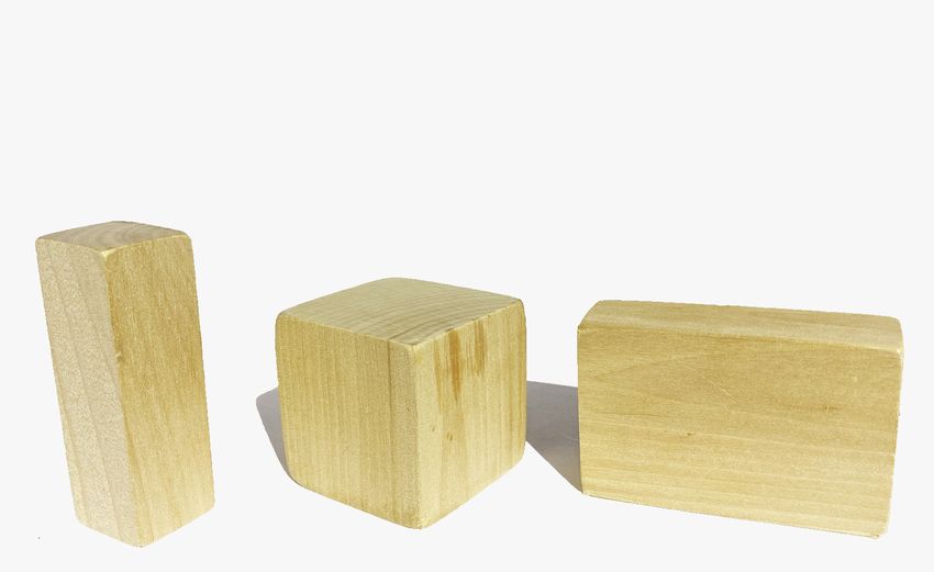
Acoustic Vibrations (Input)                     Stable Scene (Output)
     Top-down camera                                   Mic1       Mic2             Mic3          Mic4          RGB          Depth
       (Training only)

                                            Sample 1
     Contact Microphones
         (Each face)

                                            Sample 2
                (A) The Boombox

                                            Sample 3

          (B) Objects: stick, cube, block                                          (C) Data samples
Figure 2. The Boombox Overview. (A) The Boombox can sense the object through four contact microphones on each side of a storage
container. A top-down RGB-D camera is used to collect the final stabilized scene after the object movements. (B) We drop three wooden
objects with different shapes. (C) Input and output data visualizations.

key challenges. Firstly, in our setting, the speed of sound is           lating these exact features is non-trivial, especially in sit-
extremely fast for the distance it will travel. Secondly, these          uations where the signal is not broad-band and in motion
methods often assume stationary sound sources, and when                  [24, 45, 2, 5]. Furthermore, these rough approximations
they do not, they require high speeds to detect Doppler ef-              can only be used to localize the object, whereas our goal is
fects. At the scale of a small box, standard radiolocation               to not only localize objects, but also predict the 3D struc-
methods are not robust because they are sensitive to slight              ture, which includes shape and orientation of the object as
errors in the estimated signal characteristics.                          well as the environment. As such, we develop a model that
    We find that convolutional networks are able to learn                learns the necessary features for reconstruction.
robust features that permit reconstruction that is accu-                     Vision and Sound. In recent years the field has seen
rate within centimeters. Our experiments demonstrate that                a growing interest in using sound and vision conjunctively.
acoustics are pivotal for revealing the visual structure be-             There are works that, given vision, enhance sounds [30, 18],
hind containment. Given just four microphones attached to                fill in missing sounds [42], and generate sounds entirely
each face of the container, we can learn to create an image              from video [32, 43]. Further, there have been recent works
that predicts both the position and shape of objects inside              in integrating vision and sound to improve recognition of
the box from vibration alone. Our approach works on real,                environmental properties [3, 21, 8] and object properties,
natural audio. Although we use low-cost and low-power mi-                such as geometry and materials [40, 39]. Lastly, there
crophones, learning from visual synchronization enables us               have been works in using audiovisual data for representa-
to transform cheap acoustic sensors into 3D visual sensors.              tion learning [33, 4, 28]. [17] investigates vision and sound
    The main contribution of this paper is an integrated hard-           in a robot setting where they predict which robot actions
ware and software platform for using acoustic vibrations to              caused a sound. There has been work for generating a face
reconstruct the visual structure inside containers. The re-              given a voice [31] and a scene from ambient sound [37].
mainder of this paper will describe The Boombox in detail.               In contrast, our work uses sound to predict the 3D visual
In section 2, we first review background on this topic. In               structure inside a container.
section 3, we introduce our perception hardware, and in sec-
                                                                            Non-line-of-sight Imaging: Due to the importance of
tion 4, we describe our learning model. Finally, in section 5,
                                                                         sensing through occlusions and containers, the field has in-
we quantitatively and qualitatively analyze the performance
                                                                         vestigated other modalities for visual reconstruction. In
and capabilities of our approach. We will open-source all
                                                                         non-line-of-sight imaging, there has been extensive work
hardware designs, software, models, and data.
                                                                         in scene reconstruction by relying on a laser to reflect off
2. Related Work                                                          surfaces and return to the receiver [6, 11]. There are also
                                                                         audio extensions [25] as well as radio-frequency based ap-
   Audio Analysis. The primary features in audio that are                proaches [41]. However, these approaches use specialized
used for sound localization [29] are time difference of ar-              and often expensive hardware for the best results. Our ap-
rival and level (amplitude) difference. Specifically calcu-              proach only uses commodity hardware costing less than $15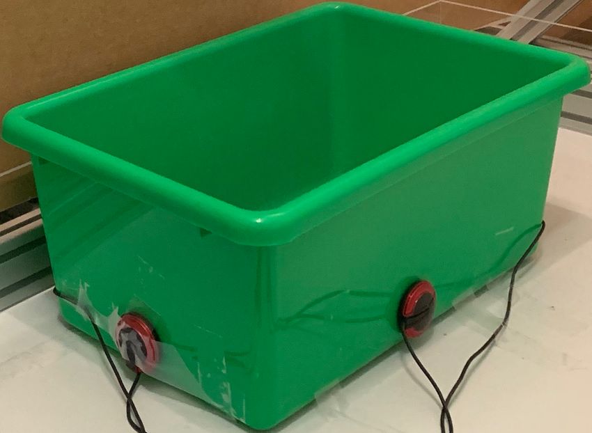
Mic1              Mic2   ...                                      ...
                                                                                                              Third
                                                                                                             Bounce

                                                                              Figure 4. Vibration Characteristics: We visualize a vibration
Figure 3. Chaotic Trajectories: We show examples of objects                   captured by two microphones in the box. There are several dis-
trajectories as they bounce around the box until becoming sta-                tinctive characteristics that need to be combined over time in order
ble. The trajectories are chaotic and sensitive to their initial condi-       to accurately reconstruct an image with the right position, orienta-
tions, making them difficult to visually predict. The moving sound            tion, and shape of objects.
source and multiple bounces also create potentially interfering vi-
brations, complicating the real-world audio signal.                           visual conditions, they allow perception despite occlusion
                                                                              and poor illumination.
at the time of writing. Due to this low-cost, a key advantage                     There is rich structure in the raw acoustic signal. For
of our approach is that it is durable, adaptable and straight-                example, the human auditory system uses inter-aural tim-
forward, which makes it easy for others to build on.                          ing difference (ITD), which is the time difference of arrival
                                                                              between both ears, and inter-aural level difference (ILD),
3. The Boombox                                                                which is the amplitude level difference between both ears,
                                                                              to locate sound sources [35].
   In this section, we present the The Boombox and discuss
                                                                                  However, in our settings, extracting these characteristics
the characteristics of the acoustic signals captured by it.
                                                                              is challenging. In practice, objects will bounce around in the
3.1. Detecting Vibrations                                                     container before arriving at their stable position, as shown
                                                                              in Figure 3. Each bounce will produce another, potentially
    The Boombox, shown in Figure 2A, is a plastic storage                     interfering vibration. In our attempts to analytically use this
container that is 15.5cm × 26cm × 13cm (width × length                        signal, we found that the third bounce has the best signal for
× height) with an open top. The box is a standard object                      the time difference of arrival, but as can be seen from Figure
that one can buy at any local hardware store.                                 4, even on the third bounce the time difference of arrival is
    When an object collides with the box, a small acoustic                    unclear in the actual waveform.
vibration will be produced in both the air and the solid box
                                                                                  There are a multitude of factors that make analytical ap-
itself. In order for the box to detect its own vibration, we
                                                                              proaches not robust to our real-world signals. Firstly, we
have attached contact microphones on each wall of the plas-
                                                                              are working with a moving signal, whereas time difference
tic cuboid storage bin. Unlike air microphones, contact mi-
                                                                              of arrival calculations work best on stationary signals due to
crophones are insensitive to the vibrations in the air (which
                                                                              the fact that it compares the time taken for a signal to travel
human ears hear as sound). Instead, they detect the vibra-
                                                                              from a fixed location. This makes it very difficult to analyt-
tion of solid objects.
                                                                              ically segment the signal into chunks of roughly the same
    The microphones are attached on the outer side of the                     location. Secondly, there are echos that make non-learning
walls, resulting in four audio channels. We arrange the mi-                   based methods difficult to identify phase shifts as the en-
crophones roughly at the horizontal center of each wall and                   vironment is a small container. Finally, the fact that the
close to the bottom. As our approach will not require cali-                   microphones are close together means that the time differ-
bration, the microphone displacements can be approximate.                     ence of arrival is encompassed in few samples, thus making
We used TraderPlus piezo contact microphones, which are                       it susceptible to noise.
very affordable (no more than $5 each).1
                                                                                  Instead of hand crafting these features, our model will
3.2. Vibration Characteristics                                                learn to identify the fraction of the signal that is most robust
                                                                              for final localization. Moreover, our model will learn to
   When objects collide with the box, the contact micro-                      identify the useful features from the signals to reconstruct
phones will capture the resulting acoustic vibrations. Fig-                   a rich 3D scene that includes the shape, orientation, and
ure 4 shows an example of the vibration captured from two                     position of the contents.
of the microphones. We aim to recover the visual structure
from this signal. As these vibrations are independent of the                  3.3. Multimodal Training Dataset
   1 We  found that these microphones gave sufficiently clear signals while      Our approach will use the visual modality in order to
being more affordable than available directional microphone arrays. Each
microphone was connected to a laptop through audio jack to USB con-
                                                                              learn the robust characteristic features of the acoustic sig-
verter. We use GarageBand software to record all four microphones to-         nal. By simply dropping objects into the box and captur-
gether to synchronize the recordings.                                         ing resulting images and vibrations, we can collect a mul-
Example 1                            Example 2                     Reconstructing a pixel requires the model to have access
                                                                           to the full spectrogram. However, we also want to take ad-
                                                                           vantage of the spatio-temporal structure of the signal. We
                                                                           thereforefore use a fully convolutional encoder and decoder
                                                                           architecture. The network transforms a spectrogram repre-
                                                                           sentation (time × frequency) into a C dimensional embed-
            Example 3                            Example 4                 ding such that the receptive field of every dimension reaches
                                                                           every magnitude in the input and every pixel in the output.
                                                                           Unlike image-to-image translation problems [44, 20, 12],
                                                                           our task requires translation across modalities.
                                                                               We use a multi-scale decoder network [27, 19, 10].
                                                                           Specifically, each decoder layer consists of two branches.
                                                                           One branch is a transposed convolutional layer to up-sample
Figure 5. Point Cloud Reconstruction from Vibration: We visu-
alize the point clouds produced by our method. These point clouds
                                                                           the intermediate feature. The other branch passes the in-
are predicted only given the acoustic vibration of the box. For each       put feature first to a convolutional layer and then a trans-
prediction, we show two different camera views.                            posed convolution so that the output for the second branch
                                                                           matches the size of the first branch. We then concatenate
timodal training dataset. We position an Intel RealSense                   the output from these two branches along the feature di-
D435i camera that looks inside the bin to capture both RGB                 mension as the input feature for the next decoder layer. We
and depth images.2                                                         perform the same operation for each decoder layer except
    We use three wooden blocks with different shapes to cre-               the last layer where only one transposed convolution layer
ate our dataset. The blocks have the same color and mate-                  is needed to predict the final output image.
rials, and we show these objects in Figure 2B. We hold the                     We use a spectrogram as the representation of audio sig-
object above the bin, and freely drop it.3 After dropping,                 nals. We apply a Fourier Transform before converting the
the objects bounce around in the box a few times before                    generated spectrogram to Mel scale. Since we have four
settling into a resting position. We record the full process               microphones, audio clips are concatenated together along
from all the microphones and the top-down camera. Over-                    a third dimension in addition to the original time and fre-
all, our collection process results diverse falling trajectories           quency dimension.
across all shapes with a total of 1,575 sequences. Figure 2C
shows an overview of the dataset.                                          4.2. Learning
    We only use the camera to collect data for learning. After                In practical applications, we often care about the resting
learning, our approach will be able to reconstruct the 3D                  position of the object so that we can localize the object. We
visual scene from the box’s vibration alone.                               therefore train the network f to predict the final stable im-
                                                                           age. For RGB image predictions, we train the network to
4. Predicting Images from Vibration                                        minimize the expected mean squared error:
   In order to create robust features, we will learn them
                                                                                    LRGB = EA,X kfRGB (A; θ) − XRGB k22

from multi-modal data. We present a convolutional network                                                                           (1)
that translates vibrations into an image.
                                                                              In order to reconstruct shape, we also train the network
4.1. Model                                                                 to predict a depth image from the acoustic vibration input.
   We will fit a model that reconstructs the visual contents               We train the model to minimize the expected L1 distance:
from the vibrations. Let Ai be a spectrogram of the vibra-
tion captured by microphone i such that i ∈ {1, 2, 3, 4}.                           Ldepth = EA,X [kfdepth (A; φ) − Xdepth k1 ]     (2)
Our model will predict the image X̂RGB = fRGB (A; θ)
where f is a neural network parameterized by θ. The net-                   Since ground truth depth often has outliers and substantial
work will learn to predict the image of a top-down view                    noise, we use an L1 loss [26]. We use stochastic gradient
into the container. We additionally have a corresponding                   descent to estimate the network parameters θ and φ.
network to produce a depth image X̂depth = fdepth (A; θ).                      After learning, we can obtain predictions for both the
                                                                           RGB image and the depth image from the acoustic vibra-
   2 The camera is 42cm away from the bottom of the bin to capture clear
                                                                           tions alone. The visual modality is only supervising repre-
top-down images.
   3 As the dynamics depend on the material properties, we wore a pow-     sentations for the audio modality, allowing reconstructions
der free disposable glove while holding the object to avoid changing the   when cameras are not viable, such during occlusions or low
humidity on the object surface.                                            illumination.
Cube (IoU Score) Stick (IoU Score) Block (IoU Score)
Random Sampling 0.07 0.03 0.09
Average Bounding Box 0.06 0.05 0.10
TDoA Search 0.06 0.04 0.06
Boombox (depth output) 0.32 Cube (IoU Score)
0.04 Stick (IoU Score)
0.19 Block (IoU Score)
Boombox (RGB output) 0.29 0.06 0.22
0 0.1
Random Sampling 0.070.2 0.3 0.4 0 0.015 0.03 0.045 0.06
0.03 0 0.06 0.12 0.18 0.24
0.09
Average Bounding BoxCube0.06
(Localization) Stick (Localization)
0.05
Block (Localization)
0.10
TDoA 17.99%
Random Sampling Search 0.06 18.36% 0.04 28.68% 0.06
Average Bounding Box 12.58% 21.38% 29.56%
Boombox (depth output) 0.32 0.04 0.19
TDoA Search 13.91% 15.99% 17.02%
Boombox
Boombox (RGB 75.15%
(depth output) output) 0.29 16.68% 0.06 65.46% 0.22
Boombox (RGB output) 89.12% 64.73% 86.73%
0 0.1 0.2 0.3 0.4 0 0.015 0.03 0.045 0.06 0 0.06 0.12 0.18 0.24
0% 25% 50% 75% 100% 0% 25% 50% 75% 100% 0% 25% 50% 75% 100%
Cube (Localization) Stick (Localization) Block (Localization)
Random Sampling 17.99% 18.36% 28.68%
Average Bounding Box Table 1
12.58% 21.38% 29.56%
All Shapes
TDoA Search (IoU
13.91% All Shapes (IoU All Shapes All Shapes 15.99% 17.02%
Score) Score Error) (Localization) (Localization
Boombox (depth output) 75.15% Error) 16.68% 65.46%
Random
Boombox Sampling
(RGB 89.12%
0.05701951823197050.000928183232211114
output) 0.209014675052411 64.73%
0.00597024354964283 86.73%
Average Bounding 0.06446263237838080.004807054024108140.213836477987421 0.013092238990353
Box 0% 25% 50% 75% 100% 0% 25% 50% 75% 100% 0% 25% 50% 75% 100%
Figure TDoA Search 0.04913837708021870.003187761697034210.156421805590541 0.00477099745227601
6. Single-shape Training Results. We show the performance of each individual model trained with one of the three objects. We
Boombox (depth 0.145518 0.03365818046676520.487311333333333 0.0693026431057607
report output)
both the mean and the standard error of the mean from three random seeds. Our approach enables robust features to be learned to
predictBoombox (RGB
the location
output)
0.229899333333333 0.01532714370361
and shape of the dropped objects. 0.86929 0.0207907316850562
Table 1
Multi-shape Training (IoU Score) Multi-shape Training (Localization)
neuralAllnetworks
All Shapes (IoU 20.90% All Shapes (IoU Shapes
on the training set, and optimize hyper-
All Shapes
Random Sampling 0.06
Average Bounding Box 0.06 Score) parameters
21.38% Score Error) on the validation set. We report results only on
(Localization (Localization)
TDoA Search 0.05 15.64% Error)
Boombox (depth output) 0.15 the testing
48.73% set. All of our results are evaluated on three ran-
Random Sampling 0.05701951823197050.000928183232211114
Boombox (RGB output) 0.23 0.209014675052411 0.00597024354964283
86.93%
dom seeds for training and evaluation. For each random
0 0.065 0.13 0.195 0.26 0% 25% 50% 75% 100%
Average Bounding 0.06446263237838080.004807054024108140.213836477987421 0.013092238990353
Box
seed, we also vary the splits of the dataset. We report the
Figure 7. Multi-shape
TDoA Search Training Results. By mixing all the train-
0.04913837708021870.00318776169703421
mean and the standard error of the mean for all outcomes.
0.156421805590541 0.00477099745227601
ing data together with all the shapes,0.145518
Boombox (depth
our model still outperforms
0.03365818046676520.487311333333333 0.0693026431057607
all the baseline methods.
output)
5.2. Evaluation Metrics
Boombox (RGB 0.229899333333333 0.01532714370361 0.86929 0.0207907316850562
Direct measurements in the pixel space is not informa-
output)
4.3. Implementation Details All vs. single tive because it is not a perceptual metric. We use two eval-
Depth output (IoU Depth output (IoU RGB outputuation RGBmetrics for our final scene reconstruction that focus
Our network RGB takesoutput (IoU
Score, in the RGB output (IoU
Multi-shape
single) input
Score, size
Training
single, (IoU
Score, 128
ofsingle)
Score) × 128
Score, × 4Score, all) (IoU
single,Multi-shape Training
output (IoU
Score,(Localization)
all, error)
where Cube
the last dimension
error)
denotes the number
error)
of micro- on the object state.
0.287593333333333 0.0405538478788114 0.31676 0.0713549652582075 0.237941 0.0228912955582102
phones.Random Sampling 0.06
The output is a 128 × 128 × 3 RGB image 20.90% or a IoU measures how well the model reconstructs both
Average Bounding Box 0.06 21.38% shape and location. Since the model predicts an image, we
128 × 128TDoA× 1 Search
depth image.0.05
We use the same 2network archi- 15.64%
tecture for both the RGB and depth output representations subtract the background to convert the predicted image into
Boombox (depth output) 0.15 48.73%
Boombox
except the(RGB 0.23
output) dimension in the last layer for different
feature 86.93% a segmentation mask. Similarly, we performed the same
modalities. All network 0 details
0.065 are0.13 listed in the Appendix.
0.195 0.26 0% 25%
operation
50%
on
75%
the ground-truth
100%
image. IoU metric then com-
Our networks are configured in PyTorch [34] and putes intersection over union with the two binary masks.
PyTorch-Lightning [15]. We optimized all the networks for Localization score evaluates whether the model pro-
500 epochs with Adam [22] optimizer and batch size of 32 duces an image with the block in the right spatial position.
on a single NVIDIA RTX 2080 Ti GPU. The learning rates With the binary masks obtained in the above process, we
starts from 0.001 and decrease by 50% at epoch 20, 50, and can fit a bounding box with minimum area around the ob-
100. ject region. We denote the distance between the center of
the predicted bounding box and the center of the ground-
5. Experiments truth bounding box as d, and the length of the diagonal
All vs. single
line of ground-truth box as l. We report the fraction of
In our experiments, weRGB testoutput
the capability
(IoU of The
RGB output (IoUBoom- Depth output timesPNthe
(IoU Depth predicted
output (IoU location
RGB output is (IoU
less than half the
RGB output (IoU diagonal:
Score, 1
box to reconstruct an image ofsingle)
its contents Score,
error)
fromsingle,
audio Score,
in- single)
N
Score,
i=1 [d
error)
i
single,
≤ l/2]. Score, all) Score, all, error)
puts. We quantitatively evaluate the model performance.
Cube 0.287593333333333 0.0405538478788114 0.31676 0.0713549652582075
5.3. Baselines 0.237941 0.0228912955582102
We then show qualitative results for our visual reconstruc-
tions. Finally, we show visualizations to analyze the learned Time Difference of Arrival (TDoA): We compare
representations. 2
against an analytical prediction of the location. In sig-
nal processing, the standard practice is to localize sound
5.1. Dataset
sources by estimating the time difference of arrival across
We partition the dataset into a training set (80%), a val- an array of microphones. In our case, the microphones
idation set (10%), and a testing set (10%). We train the surround the sound source. There are several ways to es-
Audio Input            Prediction            Ground Truth                   Audio Input          Prediction         Ground Truth

                            RGB output (IoU       RGB output (IoU        Depth output (IoU      Depth output (IoU   RGB output (IoU   RGB output (IoU
                            Score, single)        Score, single,         Score, single)         Score, single,      Score, all)       Score, all, error)
                                                  error)                                        error)
Figure 8. Model Prediction Visualizations with Unknown Shapes From left to right on each column, we visualize the audio input, the
Stick                      0.05514 0.00528312473825860.03734033333333330.00261314531636579 0.137758 0.0115488521218922
predicted scene, and the ground-truth images. Our model can produce accurate predictions for object shape, position and orientation.
Block                                  0.221466 0.00751202078893112                    0.186803 0.03136349604768790.314000333333333 0.0168611524945493

                                          Single-shape training      Multi-shape training
                                                                                                    the dataset bias. Therefore, we extracted object bounding
                    RGB Output (IoU Score)                 RGB Output (Localization)
                                                                                                    boxes from all the training data through background sub-
Cube        0.288                                    89.12%                                         traction and rectangle fitting to obtain the average center
            0.238                                    81.89%
            0.055                                    64.73%
                                                                                                    location, box sizes and box orientation. This baseline uses
Stick
            0.138                                    82.41%                                         the average bounding box as the prediction for all the test
            0.221                                    86.73%
Block       0.314                                    98.07%                                         samples.
        0            0.1      0.2      0.3      0.4 0%     25%       50%      75%        100%
                                                                                                    5.4. Reconstruction via Single Shape Training
                    Depth Output (IoU Score)              Depth Output (Localization)
                                                                                                        In this experiment, we train separate models for each
Cube        0.317                                    75.15%
            0.178                                    48.30%                                         shape of the object independently. Figure 6 shows The
Stick
            0.037                                    16.68%                                         Boombox is able to reconstruct both the position and ori-
            0.063                                    30.42%
            0.187                                    65.46%
                                                                                                    entation of the shapes. The convolutional network obtains
Block       0.195                                    67.39%                                         the best performance for most shapes on both evaluation
        0            0.1      0.2      0.3      0.4 0%     25%       50%      75%        100%
                                                                                                    metrics.
                                                                                                        Our model performs significantly better than the analyt-
Figure 9. Performance before and after multi-shape training.
                                                                                                    ical TDoA baseline. Our method outperforms TDoA of-
Multi-shape training enables shape knowledge transfer to improve
the overall performance
                                                                                                    ten by significant margins, suggesting that our learning-
                                                                                                    based model is learning robust acoustic features for local-
                                                                                                    ization. Due to the realistic complexity of the audio signal,
timate the time difference of arrival, and we use the Gen-
                                                                                                    the hand-crafted features are hard to reliably estimate. Our
eralized Cross Correlation with Phase Transform (GCC-
                                                                                                    model outperforms both the random sampling and average
PHAT), which is the established, textbook approach [23].
                                                                                                    bounding box baseline, indicating that our model learns the
Once we have our time difference of arrival estimate, we
                                                                                                    natural correspondence between acoustic signals and visual
find the location in the box that would yield a time differ-
                                                                                                    scene rather than memorizing the training data distribution.
ence of arrival that is closest to our estimate.
                                                                                                        These results highlight the relative difficulty at recon-
   Random Sampling: To evaluate if the learned mod-                                                 structing different shapes from sound. By comparing
els simply memorize the training data, we compared our                                              the model performance across various shapes, the model
method against a random sampling procedure. This base-                                              trained on cubes achieves the best performance while the
line makes a prediction by randomly sampling an image                                               model trained on blocks performs slightly worse. The most
from the training set and using it as the prediction. We                                            difficult shape is the stick.
repeated this step for all testing examples over 10 random
seeds.                                                                                              5.5. Reconstruction via Multiple Shape Training
   Average Bounding Box: The average bounding box                                                      We next analyze how well The Boombox reconstructs its
baseline aims to measure to what extent the model learns                                            contents when the shape is not known a priori. We train
Mic 1 (Before, After) Mic 2 (Before, After) Mic 3 (Before, After) Mic 4 (Before, After)
(A) Remove amplitude
Mic2 Ground Truth Before Flipping Prediction Before Flipping Prediction After Flipping
(B) Flip microphones Mic4 Mic1
Cube (IoU Score) Stick (IoU Score) Block (IoU Sco
Mic3 Random Sampling 0.07 0.03 0.09
Average Bounding Box 0.06 0.05 0.10
Mic 1 (Before, Shift 0.01s) Mic 2 (Before, Shift 0.01s) Mic 3 (Before, Shift 0.01s) Mic 4 0.04
(Before, Shift 0.01s)
TDoA Search 0.06 0.06
Boombox (depth output) 0.32 0.04 0.19
Boombox (RGB output) 0.29 0.06 0.22
0 0.1 0.2 0.3 0.4 0 0.015 0.03 0.045 0.06 0 0.06 0.12
Cube (Localization) Stick (Localization) Block (Localizat
Random Sampling 17.99% 18.36% 28.68%
(C) Temporal Shift
Average Bounding Box 12.58% 21.38% 29.56%
TDoA Search 13.91% 15.99% 17.02%
Boombox (depth output) 75.15% 16.68% 65.46%
Boombox (RGB output) 89.12% 64.73% 86.73%
0% 25% 50% 75% 100% 0% 25% 50% 75% 100% 0% 25% 50%
100 200 300 400 500 Table 1 600
Temporal Shift
RGB output (IoU RGB output (IoU RGB output RGB output Depth output (IoU Depth outpu
Score) Score Error)
(Localization (Localization)
Figure 10. Visualization of Ablation Studies: We visualize the impact of different ablations on the model. A) By thresholding Error) theScore) Score Error
spectrograms, we remove the amplitude from the input. B) Since the differencesOriginal between the signals0.01532714370361
0.229899333333333 from the microphones 0.86929 are important
0.0207907316850562 0.145518 0.03365818
for location, we experimented with flipping the microphones only at testingNotime.amplitudeThe model’s 0.111411 0.00396026543723187
predictions show0.745501333333333
a corresponding 0.0218479440248073
flip as 0.068995 0.01404424
Flipped mics 0.00114333333333333
0.000187631139325125
0.08601966666666670.01161389566185460.005083666666666670.00209377
well in the predicted images. C) We also experimented with shifting the relative time difference between the microphones, introducing an
Temporal shift 100 0.217426666666667 0.0173902832000453 0.871465 0.01869963365951320.133801333333333 0.03087322
artificial delay in the microphones only at testing time. A shift in time causes a shift in space in the model’s predictions.
Temporal shift 300 0.171590333333333 0.0255842748730109
The corruptions
0.823479 0.02965312112296670.09645266666666670.01574137
are consistent with a block falling in that location. Temporal shift 500 0.132887666666667 0.02856062771446810.728956333333333 0.06198781147487340.06308633333333330.01164863
RGB output (IoU Score) RGB output (Localization)
a single model with all the object shapes. The training
Original 0.23 86.93%
data for each shape are simply combined together so that No amplitude 0.11 74.55%
Flipped mics 0.00 8.60%
the training, validation and testing data are naturally well- Temporal shift 100 0.22 87.15%
Temporal shift 300 0.17 82.35%
balanced with respect to the shapes. This setting is chal- Temporal shift 500 0.13 72.90%
0 0.075 0.15 0.225 0.3 0% 25% 50% 75% 100%
lenging because the model needs to learn audio features for
Depth output (IoU Score) Depth output (Localization)
multiple shapes at once.
Original 0.15 48.73%
We show qualitative predictions for both RGB and depth No amplitude 0.07 25.96%
Flipped mics 0.01 3.98%
images in Figure 8. Moreover, since we are predicting a Temporal shift 100 0.13 46.22%
Temporal shift 300 0.10 36.81%
depth image, our model is able to produce a 3D point cloud. Temporal shift 500 0.06 25.15%
We visualize several examples from multiple viewpoints in 0 0.045 0.09 0.135 0.18 0% 25% 50% 75% 100%
Figure 5. While analytical approaches are able to predict a All vs. single
3D scalar position, we are able to predict a 3D point cloud. Figure 11. Quantitative
RGB output (IoU
performance
RGB output (IoU
under the ablation stud-
Depth output (IoU Depth output (IoU RGB output (IoU RGB outpu
Score, single) Score, single, Score, single) Score, single,
ies. We experiment with different
error)
perturbations to our input dataScore, all)
error)
Score, all, e
Figure 7 shows the convolutional networks are able to
to understand
Cube the0.287593333333333
model decisions.0.0405538478788114 0.31676 0.0713549652582075 0.237941 0.02289129
learn robust features even when shapes are unknown. When
the training data combines all shapes, the model should be
able to share features between shapes, thus improving per- smaller surface area of these two shapes, the
2 cube perfor-
formance. To validate this, we compare performance on the mance slightly degrades.
multi-shape versus the single-shape models. We use both
5.6. Ablations
IoU and the localization model. Figure 9 shows that the
performance on the block and stick shapes are improved Since the model generalizes to unseen examples, our re-
by a large margin. We notice that the performance of the sults suggest that the convolutional network are learning ro-
cube drops due to the confusion between shapes. When the bust acoustic features. To better understand what features
cube confuses with the stick or the block, because of the the model has learned specifically, we perform several ab-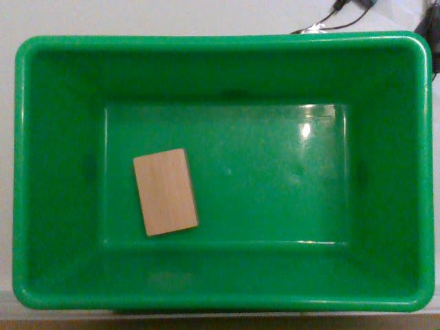
lation studies in Figure 10 and Figure 11.                                   Angle and
                                                                          Relative Position
    Flip microphones. The microphones’ layout should
matter for our learned model to localize the objects. When
we flipped the microphone location, due to the symmetric
nature of the hardware setup, the predictions should also
be flipped accordingly. To study this, we flipped the cor-
responding audio input with a pair-wise strategy, shown in
Figure 10. Specifically, the audio input of the Mic1 and
Mic4 are flipped, and the audio input of the Mic2 and Mic3
are flipped. Our results in Figure 10B shows that our model
indeed produces a flipped scene. The performance in Figure
11 nearly drops to zero, suggesting that the model implicitly
learned the relative microphone locations to assist its final     Figure 12. t-SNE embeddings on the latent features from the en-
                                                                  coder network. The color encoding follows a color wheel denoting
prediction.
                                                                  the angle and relative position to the center of the container. Our
    Remove amplitude. The relative amplitude between mi-          model learns to encode the position and orientation of the objects
crophones is another signal that can indicate the position        in its internal representations.
of the sound source with respect to different microphones.
We removed the amplitude information by thresholding the          transitions between colors suggest the features are able to
spectrograms, shown in Figure 10. We retrained the net-           smoothly interpolate spatially.
work due to potential distribution shift. As expected, even
though the time and frequency information are preserved,          6. Conclusion
the model performs much worse (Figure 11), suggesting
that our model additionally learns to use amplitude for the           We have introduced The Boombox, a low-cost container
predictions.                                                      integrated with a convolutional network that uses acoustic
    Temporal shift. We are interested to see if our model         vibrations to reconstruct a 3D point cloud from image and
learns to capture features about the time difference of ar-       depth. Containers are ubiquitous, and this paper shows that
rival between microphones. If time difference of arrival in-      we can equip them with sound perception to localize and
formation is helpful, when we shift the audio signal tempo-       reconstruct their contents inside.
rally, the model prediction should also shift spatially. We           Acknowledgements: We thank Philippe Wyder, Dı́dac
experimented with various degrees of temporal shifts on           Surı́s, Basile Van Hoorick and Robert Kwiatkowski for
the original spectrograms. For example, shifting 500 sam-         helpful feedback. This research is based on work par-
ples corresponds to shifting about 0.01s (500 / 44,000). By       tially supported by NSF NRI Award #1925157, NSF CA-
shifting the Mic1’s spectrogram forward and Mic4’s spec-          REER Award #2046910, DARPA MTO grant L2M Pro-
trogram backward with zero padding to maintain the same           gram HR0011-18-2-0020, and an Amazon Research Award.
amount of time, and preforming similar operation on Mic2          MC is supported by a CAIT Amazon PhD fellowship. We
and Mic3 respectively, we should expect that the predicted        thank NVidia for GPU donations. The views and conclu-
object position shifts towards the left-up direction. In Fig-     sions contained herein are those of the authors and should
ure 10, we can clearly observe this trend as temporal shift       not be interpreted as necessarily representing the official
increases. Shifting the signal in time decreases the model’s      policies, either expressed or implied, of the sponsors.
performance, demonstrating that the model has picked up
on the time difference of arrival.                                References
                                                                   [1] Andréa Aguiar and Renée Baillargeon. 2.5-month-old in-
5.7. Feature Visualization                                             fants’ reasoning about when objects should and should not
                                                                       be occluded. Cognitive psychology, 39(2):116–157, 1999.
    We finally visualize the latent features in between our en-
                                                                   [2] Inkyu An, Myungbae Son, Dinesh Manocha, and Sung-Eui
coder and decoder network by projecting them into a plane
                                                                       Yoon. Reflection-aware sound source localization. In 2018
with t-SNE[36], shown in Figure 12. We colorize the points
                                                                       IEEE International Conference on Robotics and Automation
according to their ground truth position and orientation. The          (ICRA), pages 66–73. IEEE, 2018.
magnitude distance from the center of the image is repre-          [3] Relja Arandjelovic and Andrew Zisserman. Look, listen and
sented by saturation, and the angle from the horizontal axis           learn. In Proceedings of the IEEE International Conference
is represented by hue. We find that there is often clear clus-         on Computer Vision, pages 609–617, 2017.
tering of the embeddings by their position and orientation,        [4] Yusuf Aytar, Carl Vondrick, and Antonio Torralba. Sound-
showing that the model is robustly discriminating the loca-            net: Learning sound representations from unlabeled video.
tion of the impact from sound alone. Moreover, the gradual             arXiv preprint arXiv:1610.09001, 2016.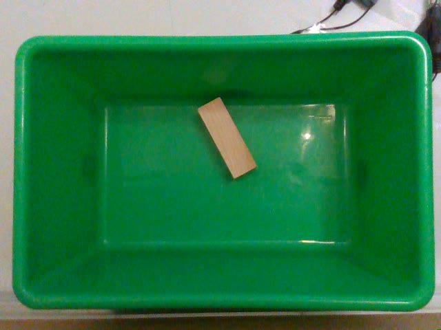
[5] Paolo Bestagini, Marco Compagnoni, Fabio Antonacci, Au-                ceedings of the IEEE conference on computer vision and pat-
     gusto Sarti, and Stefano Tubaro. Tdoa-based acoustic source            tern recognition, pages 2462–2470, 2017.
     localization in the space–range reference frame. Multidimen-    [20]   Phillip Isola, Jun-Yan Zhu, Tinghui Zhou, and Alexei A
     sional Systems and Signal Processing, 25(2):337–359, 2014.             Efros. Image-to-image translation with conditional adver-
 [6] Katherine L Bouman, Vickie Ye, Adam B Yedidia, Frédo                  sarial networks. In Proceedings of the IEEE conference on
     Durand, Gregory W Wornell, Antonio Torralba, and                       computer vision and pattern recognition, pages 1125–1134,
     William T Freeman. Turning corners into cameras: Princi-               2017.
     ples and methods. In Proceedings of the IEEE International      [21]   Evangelos Kazakos, Arsha Nagrani, Andrew Zisserman, and
     Conference on Computer Vision, pages 2270–2278, 2017.                  Dima Damen. Epic-fusion: Audio-visual temporal bind-
 [7] Rodney A Brooks. Planning collision-free motions for pick-             ing for egocentric action recognition. In Proceedings of the
     and-place operations. The International Journal of Robotics            IEEE/CVF International Conference on Computer Vision,
     Research, 2(4):19–44, 1983.                                            pages 5492–5501, 2019.
 [8] Fanjun Bu and Chien-Ming Huang.               Object perma-     [22]   Diederik P Kingma and Jimmy Ba. Adam: A method for
     nence through audio-visual representations. arXiv preprint             stochastic optimization. arXiv preprint arXiv:1412.6980,
     arXiv:2010.09948, 2020.                                                2014.
 [9] Ming-Fang Chang, John Lambert, Patsorn Sangkloy, Jag-           [23]   Charles Knapp and Glifford Carter. The generalized correla-
     jeet Singh, Slawomir Bak, Andrew Hartnett, De Wang, Peter              tion method for estimation of time delay. IEEE transactions
     Carr, Simon Lucey, Deva Ramanan, et al. Argoverse: 3d                  on acoustics, speech, and signal processing, 24(4):320–327,
     tracking and forecasting with rich maps. In Proceedings of             1976.
     the IEEE/CVF Conference on Computer Vision and Pattern          [24]   Zhiwei Liang, Xudong Ma, and Xianzhong Dai. Ro-
     Recognition, pages 8748–8757, 2019.                                    bust tracking of moving sound source using multiple model
[10] Boyuan Chen, Carl Vondrick, and Hod Lipson. Visual behav-              kalman filter. Applied acoustics, 69(12):1350–1355, 2008.
     ior modelling for robotic theory of mind. Scientific Reports,   [25]   David B Lindell, Gordon Wetzstein, and Vladlen Koltun.
     11(1):1–14, 2021.                                                      Acoustic non-line-of-sight imaging. In Proceedings of the
[11] Wenzheng Chen, Simon Daneau, Fahim Mannan, and Felix                   IEEE/CVF Conference on Computer Vision and Pattern
     Heide. Steady-state non-line-of-sight imaging. In Proceed-             Recognition, pages 6780–6789, 2019.
     ings of the IEEE/CVF Conference on Computer Vision and          [26]   Fangchang Ma and Sertac Karaman. Sparse-to-dense: Depth
     Pattern Recognition, pages 6790–6799, 2019.                            prediction from sparse depth samples and a single image. In
[12] Yunjey Choi, Minje Choi, Munyoung Kim, Jung-Woo Ha,                    2018 IEEE International Conference on Robotics and Au-
     Sunghun Kim, and Jaegul Choo. Stargan: Unified genera-                 tomation (ICRA), pages 4796–4803. IEEE, 2018.
     tive adversarial networks for multi-domain image-to-image       [27]   Michael Mathieu, Camille Couprie, and Yann LeCun. Deep
     translation. In Proceedings of the IEEE conference on                  multi-scale video prediction beyond mean square error.
     computer vision and pattern recognition, pages 8789–8797,              arXiv preprint arXiv:1511.05440, 2015.
     2018.                                                           [28]   Carolyn Matl, Yashraj Narang, Dieter Fox, Ruzena Ba-
[13] Achal Dave, Tarasha Khurana, Pavel Tokmakov, Cordelia                  jcsy, and Fabio Ramos. Stressd: Sim-to-real from sound
     Schmid, and Deva Ramanan. Tao: A large-scale benchmark                 for stochastic dynamics. arXiv preprint arXiv:2011.03136,
     for tracking any object. In European conference on computer            2020.
     vision, pages 436–454. Springer, 2020.                          [29]   John C Middlebrooks. Sound localization. Handbook of clin-
[14] Ivan Dokmanić, Reza Parhizkar, Andreas Walther, Yue M                 ical neurology, 129:99–116, 2015.
     Lu, and Martin Vetterli. Acoustic echoes reveal room            [30]   Arun Asokan Nair, Austin Reiter, Changxi Zheng, and Shree
     shape. Proceedings of the National Academy of Sciences,                Nayar. Audiovisual zooming: what you see is what you hear.
     110(30):12186–12191, 2013.                                             In Proceedings of the 27th ACM International Conference on
[15] WA Falcon and .al. Pytorch lightning. GitHub. Note:                    Multimedia, pages 1107–1118, 2019.
     https://github.com/PyTorchLightning/pytorch-lightning, 3,       [31]   Tae-Hyun Oh, Tali Dekel, Changil Kim, Inbar Mosseri,
     2019.                                                                  William T Freeman, Michael Rubinstein, and Wojciech Ma-
[16] Lisa Feigenson and Susan Carey. Tracking individuals via               tusik. Speech2face: Learning the face behind a voice. In
     object-files: evidence from infants’ manual search. Develop-           Proceedings of the IEEE/CVF Conference on Computer Vi-
     mental Science, 6(5):568–584, 2003.                                    sion and Pattern Recognition, pages 7539–7548, 2019.
[17] Dhiraj Gandhi, Abhinav Gupta, and Lerrel Pinto. Swoosh!         [32]   Andrew Owens, Phillip Isola, Josh McDermott, Antonio Tor-
     rattle!     thump!–actions that sound.        arXiv preprint           ralba, Edward H Adelson, and William T Freeman. Visually
     arXiv:2007.01851, 2020.                                                indicated sounds. In Proceedings of the IEEE conference on
[18] Ruohan Gao and Kristen Grauman. 2.5 d visual sound. In                 computer vision and pattern recognition, pages 2405–2413,
     Proceedings of the IEEE/CVF Conference on Computer Vi-                 2016.
     sion and Pattern Recognition, pages 324–333, 2019.              [33]   Andrew Owens, Jiajun Wu, Josh H McDermott, William T
[19] Eddy Ilg, Nikolaus Mayer, Tonmoy Saikia, Margret Keuper,               Freeman, and Antonio Torralba. Ambient sound provides
     Alexey Dosovitskiy, and Thomas Brox. Flownet 2.0: Evolu-               supervision for visual learning. In European conference on
     tion of optical flow estimation with deep networks. In Pro-            computer vision, pages 801–816. Springer, 2016.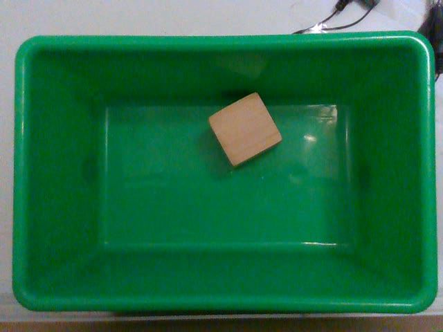
[34] Adam Paszke, Sam Gross, Francisco Massa, Adam Lerer,            based sound source localization in multimedia surveillance.
     James Bradbury, Gregory Chanan, Trevor Killeen, Zeming          Multimedia Tools and Applications, 77(3):3369–3385, 2018.
     Lin, Natalia Gimelshein, Luca Antiga, Alban Desmaison,
     Andreas Kopf, Edward Yang, Zachary DeVito, Martin Rai-
     son, Alykhan Tejani, Sasank Chilamkurthy, Benoit Steiner,
     Lu Fang, Junjie Bai, and Soumith Chintala. Pytorch: An im-
     perative style, high-performance deep learning library. In H.
     Wallach, H. Larochelle, A. Beygelzimer, F. d'Alché-Buc, E.
     Fox, and R. Garnett, editors, Advances in Neural Informa-
     tion Processing Systems 32, pages 8024–8035. Curran Asso-
     ciates, Inc., 2019.
[35] John W Strutt. On our perception of sound direction. Philo-
     sophical Magazine, 13(74):214–32, 1907.
[36] Laurens Van der Maaten and Geoffrey Hinton. Visualiz-
     ing data using t-sne. Journal of machine learning research,
     9(11), 2008.
[37] Chia-Hung Wan, Shun-Po Chuang, and Hung-Yi Lee. To-
     wards audio to scene image synthesis using generative ad-
     versarial network. In ICASSP 2019-2019 IEEE Interna-
     tional Conference on Acoustics, Speech and Signal Process-
     ing (ICASSP), pages 496–500. IEEE, 2019.
[38] Andy Zeng, Shuran Song, Kuan-Ting Yu, Elliott Donlon,
     Francois R Hogan, Maria Bauza, Daolin Ma, Orion Taylor,
     Melody Liu, Eudald Romo, et al. Robotic pick-and-place of
     novel objects in clutter with multi-affordance grasping and
     cross-domain image matching. In 2018 IEEE international
     conference on robotics and automation (ICRA), pages 3750–
     3757. IEEE, 2018.
[39] Zhoutong Zhang, Qiujia Li, Zhengjia Huang, Jiajun Wu,
     Joshua B Tenenbaum, and William T Freeman. Shape and
     material from sound. 2017.
[40] Zhoutong Zhang, Jiajun Wu, Qiujia Li, Zhengjia Huang,
     James Traer, Josh H McDermott, Joshua B Tenenbaum, and
     William T Freeman. Generative modeling of audible shapes
     for object perception. In Proceedings of the IEEE Interna-
     tional Conference on Computer Vision, pages 1251–1260,
     2017.
[41] Mingmin Zhao, Tianhong Li, Mohammad Abu Alsheikh,
     Yonglong Tian, Hang Zhao, Antonio Torralba, and Dina
     Katabi. Through-wall human pose estimation using radio
     signals. In Proceedings of the IEEE Conference on Computer
     Vision and Pattern Recognition, pages 7356–7365, 2018.
[42] Hang Zhou, Ziwei Liu, Xudong Xu, Ping Luo, and Xiaogang
     Wang. Vision-infused deep audio inpainting. In Proceedings
     of the IEEE/CVF International Conference on Computer Vi-
     sion, pages 283–292, 2019.
[43] Yipin Zhou, Zhaowen Wang, Chen Fang, Trung Bui, and
     Tamara L Berg. Visual to sound: Generating natural sound
     for videos in the wild. In Proceedings of the IEEE Con-
     ference on Computer Vision and Pattern Recognition, pages
     3550–3558, 2018.
[44] Jun-Yan Zhu, Taesung Park, Phillip Isola, and Alexei A
     Efros. Unpaired image-to-image translation using cycle-
     consistent adversarial networks. In Proceedings of the IEEE
     international conference on computer vision, pages 2223–
     2232, 2017.
[45] Mengyao Zhu, Huan Yao, Xiukun Wu, Zhihua Lu, Xiao-
     qiang Zhu, and Qinghua Huang. Gaussian filter for tdoa
You can also read