The Impact of COVID on Potential Output - Federal Reserve ...
←
→
Page content transcription
If your browser does not render page correctly, please read the page content below
FEDERAL RESERVE BANK OF SAN FRANCISCO

                                  WORKING PAPER SERIES

                         The Impact of COVID on Potential Output
                                        John Fernald
                            Federal Reserve Bank of San Francisco

                                          Huiyu Li
                            Federal Reserve Bank of San Francisco

                                          March 2021

                                   Working Paper 2021-09

        https://www.frbsf.org/economic-research/publications/working-papers/2021/09/

Suggested citation:
Fernald, John, Huiyu Li. 2021 “The Impact of COVID on Potential Output,” Federal
Reserve Bank of San Francisco Working Paper 2021-09.
https://doi.org/10.24148/wp2021-09

The views in this paper are solely the responsibility of the authors and should not be interpreted
as reflecting the views of the Federal Reserve Bank of San Francisco or the Board of Governors
of the Federal Reserve System.
The Impact of COVID on Potential Output
John Fernald Huiyu Li∗
Draft: March 22, 2021
Abstract
The level of potential output is likely to be subdued post-COVID relative to
its pre-pandemic estimates. Most clearly, capital input and
full-employment labor will both be lower than they previously were.
Quantitatively, however, these effects appear relatively modest. In the long
run, labor scarring could lead to lower levels of employment, but the slow
pre-recession pace of GDP growth is unlikely to be substantially affected.
Keywords: Growth accounting, productivity, potential output.
JEL codes: E01, E23, E24, O47
∗
Fernald: Federal Reserve Bank of San Francisco and INSEAD; Li: Federal Reserve Bank of
San Francisco. We thank Mitchell Ochse for excellent research support. Any opinions and
conclusions expressed herein are those of the authors and do not necessarily represent the
views of the Federal Reserve System.
12
1 Introduction
How will COVID-19 affect the level and growth rate of U.S. GDP going forward?
The answer to this question matters directly for well-being. But it also matters
for policy makers. For example, the level and growth of potential output has
important implications for monetary policymakers assessing the degree of
slack and inflationary pressures.
This paper provides a simple growth-accounting framework to think
through the short-, medium-, and longer-run channels through which
COVID-19 might affect potential output. We can quantify some of the
channels. These ”known knowns” suggest a relatively modest impact so far. We
discuss a range of other channels that are ”known unknowns”: The
importance—and, in some cases, even the sign—of these channels is
necessarily speculative.1
Even before the coronavirus wreaked its havoc, the normal pace of growth
appeared subdued relative to history (See, for example, (Fernald and Li, 2019)).
We argue that COVID-19 has not yet caused changes that push this sluggish
”longer-run” growth-rate prediction substantially off course. Labor-supply
growth will remain low and COVID does not, on its own, seem likely to lead to
sharp changes in research effort or in the idea production function that would
push us away from the slow-productivity-growth trajectory. Our point forecast
is that longer-run (say, 5 to 10 years out) GDP growth is likely to be a little
above 1 1/2 percent.
Of course, even if the growth rate isn’t much affected, there can be
important changes in the level of potential. After the Great Recession, for
example, potential output appeared to be harmed for a time by the substantial
reduction in capital accumulation and, potentially, by disruptions to labor
markets. In the near term, our best guess is that COVID-19 will modestly
reduce the level of potential output through headwinds to labor, capital, and
1
By definition, we do not discuss unknown unknowns. Historically, unanticipated factors
have probably been the most important determinants of changes in potential output.3
total factor productivity (TFP). Labor supply is held back by child care
demands and other sources. Investment has fallen, which hits the economy’s
productive capacity; and much of the apparent strength in investment in
information technology equipment reflects the need to duplicate idle office
capital to allow workers to work from home. The level of TFP is likely to be held
down by adjustment costs associated with the transition to work-for-home, as
well as from the need to adjust supply chains.2
Depending in part on how long the downturn continues, there is the risk of
hysteresis. It follows that the ultimate effect on the level of potential output may
depend on the countercyclical effects of monetary and fiscal policy that seek to
limit the depth of the pandemic-induced downturn.3
Throughout this paper, we focus on a production-function definition of
potential output: the level of output given actual capital and technology, if
capital and labor input (both hours and labor quality) were utilized at
“normal” levels. This is the definition used by the Congressional Budget Office
(CBO) and many policy organizations. It is related to, but conceptually a little
different than, the flexible-price equilibrium level, because labor supply or
factor utilization might optimally vary in response to some shocks in a way not
allowed for with the production-function approach. Nevertheless, Kiley (2013)
argues that the output gap in a carefully specified dynamic stochastic general
equilibrium model, the natural-rate measure of the output gap comoves
reasonably closely with a production-function based measure. (See Fernald
(2015) for further discussion.) In any case, in the long run, the two approaches
are equivalent.
2
Bloom et al. (2020b) suggest that the level of U.K. TFP might persistently be reduced, based
on a large survey of firms.
3
After the Great Recession, the persistence of the adverse effects on the level of potential
output are controversial. Fernald et al. (2017) argue that temporary effects through capital
accumulation and labor-market disruptions were not persistent. They find that, by 2016, most
of the disappointing U.S. output performance relative to pre-Great-Recession trends reflected
non-recession factors. Cerra et al. (2020) and others, in contrast, interpret the evidence as
favoring hysteresis. Jordá et al. (2020b) discuss additional references on the persistent effects of
demand shocks on potential output.4
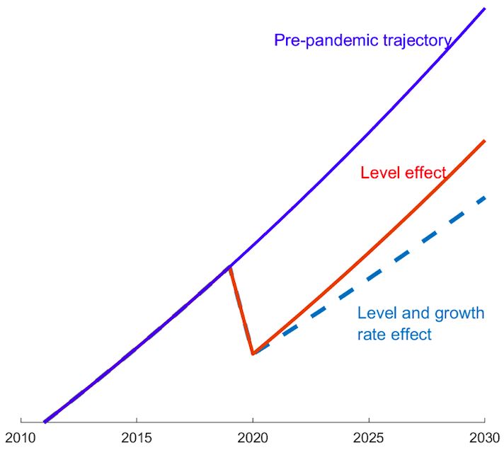
Figure 1: Level and growth rate effects on potential output
Notes: Figure shows a stylized representation of possible potential output paths following
COVID-19.
Figure 1 motivates the organization of the paper. Section 2 discusses the
growth-accounting framework we use to understand potential output at a
point in time, as well as over time. The framework thus describes the position
and slope of the lines in the figure. Section 3 provides background facts on the
pre-pandemic trajectory of the economy—the blue line in the figure. We then
discuss possible effects on the level of potential in Section 4—the red line in
the figure. These level effects may come through capital, labor, or TFP. For a
number of the channels we can quantify the likely effects, which are most
likely modestly negative. As shown, the level effects are permanent, though
many of them are likely to be temporary. In the red line, the longer-run growth
rate is unchanged from its pre-pandemic trajectory. But the pandemic might
also affect the growth rate. So, in Section 5, we then discuss potential reasons
why the longer-run growth rate of the economy might change. The dashed line
shows a post-COVID change in the growth rate. In the figure, the growth-rate
change is also associated with a level effect on the ”jumping off point” for the5
change in growth. Such a level effect might or might not occur in practice.
2 Potential output accounting framework
A standard way to think about potential output growth is in terms of growth in
inputs as well as in the efficiency with which those inputs are used. The
following constant-returns aggregate production function, in growth-rate
terms, provides the organizing framework for the rest of the paper:
dy = α dk + (1 − α) (dh + dlq) + dtf p (1)
All variables, including factor shares, have time subscripts that we omit for
simplicity. dy is output growth, α is capital’s output elasticity (and, under
standard conditions, its factor share), and dk is capital-input growth,
“Effective” labor growth is the sum of hours growth, dh, and labor-quality
growth, dlq. In the growth-accounting literature, labor quality captures the
effect of education and experience on the labor force (Jorgenson et al., 1987;
Bosler et al., 2017).4 dtf p is total-factor-productivity growth, which is defined
implicitly by this equation as output growth not explained by share-weighted
input growth. In that sense, it is a broad measure of technology or efficiency.
This measure of technology reflects any changes in factor misallocation as well
as any mismeasurement of factor shares or factor inputs.
By estimating or projecting the variables on the right-hand side of (1), we
can estimate potential growth. In particular, we can estimate what labor and
TFP growth would be if the economy were at “full employment,” and we can
estimate what actual capital input is based on investment flows (and project it
using estimates of future investment). For this reason, (1) provides a useful
4
More formally, suppose the production function has N types of labor, so that Y =
F (K, H1 , H2 , ...HN ). Then P the standard Solow accounting that leads to equation (1) would
imply dy = αdk P + (1 − α) i sLi dhi /(1 − α) + dtf p, where
P sLi is the revenue share of labor
input i. If H = i Hi is total hours worked, then dlq ≡ i sLi dhi /(1 − α) − dh.6
organizing framework for thinking about how COVID might affect potential
over the next few years.
It will be useful in the long run to write growth in output identically as the
sum of growth in labor productivity and hours:
dy = (dy − dh) + dh. (2)
In standard growth models, steady-state labor-productivity growth, dy − dh,
depends solely on TFP growth. The reason is that capital growth from equation
(1) is endogenous and depends on growth in technology and in labor input.
Specifically, rearranging the production function (1), labor productivity is:
dy − dh = α (dk − dh − dlq) + dlq + dtf p. (3)
In the standard one-sector model, steady-state capital per quality-adjusted
hour grows at the rate of labor-augmenting technical progress: dk − dh − dlq =
dtf p/(1 − α). It then follows from equation (3) that
dtf p
dy − dh = + dlq. (4)
1−α
Thus, in the long run, labor productivity depends primarily on technology,
whereas hours growth dh depends primarily on demographics. Of course,
there are models where TFP growth itself depends on demographics. Perhaps
most obviously, in semi-endogenous growth models such as Jones (2002),
steady-state TFP growth depends completely on demographics: TFP comes
from ideas, and ideas come from people. However, even in that model, other
factors—most importantly, rising research effort, though also changes in the
idea production function—can matter for very long periods: according to that
model, the economy has been growing faster than steady-state for at least a
century and a half (Fernald and Jones, 2014). In any case, although we assume
in what follows that TFP growth is largely independent of demographics over7
the next decade or two, allowing for demographics to affect TFP growth would
reinforce the slow-growth message of our paper. That is, U.S. and advanced
economy growth in the working age population is expected to be slow (or even
negative) in coming decades which, through reduced idea-creation, lower
firm-dynamism, or other channels, could put downward pressure on TFP
growth 5
However, in the quarters or even years immediately following the COVID
recession (or other downturns), equation (2) is less useful as a guide to
near-term potential output. The reason is that observed labor productivity
growth is substantially affected by the business cycle. Because the forces do
not all act in the same direction, it can be more challenging to easily assess the
full-employment level and growth rate of labor productivity. (see, e.g., Fernald
and Wang 2016).6 Of course, one can calculate the implied potential (or
structural) growth in labor productivity. But one needs to use (1) to estimate
potential output growth first.
Thus, in thinking about potential output in the near term, we continue to
focus on equation (1). For the longer-term, however, where capital is
endogenous to other supply-side impulses, we think about equation (4).
5
In addition to Jones (2002) and Fernald and Jones (2014), Peters and Walsh (2019)) is
another recent example, with references. Those authors write down a model of firm dynamics,
in which lower population growth leads to reduced creative destruction and productivity
growth.
6
On one hand, measured TFP tends to be procyclical because of fluctuations in factor
utilization: Variations in capital’s workweek and labor effort. On the other hand, capital
deepening rises sharply (countercyclically), because labor falls. Ceteris paribus, the capital-
deepening effect raises labor productivity. (Note that this is the effect of diminishing marginal
product of labor; it’s why we typically draw labor demand curves as downward sloping). In
addition, another countercyclical force is that, in downturns, including during COVID, workers
with less education and experience disproportionately lose jobs. That, in turn, provides a
countercyclical boost to the level of skills—the “quality”—of the people who keep their jobs.
Higher workforce skills again works to raise the level of labor productivity.8
3 Longer-run growth before COVID
We start with some background on longer-run growth in the U.S. before the
pandemic. So, in this section, we use the decomposition in equation (2) that
focuses on labor productivity and hours. The section establishes some “facts”
about pre-pandemic growth in productivity, hours, and GDP. These include
discussing why, prior to the pandemic, the outlook for longer-run U.S. growth
appeared likely to be slow.
Table 1 shows total-economy output, hours worked, and output per hour for
selected periods since World War II. The periods highlight notable variations
in productivity growth.7 Column (3) highlights how productivity growth has
shifted between normal and exceptional periods (Fernald, 2016). Productivity
growth was fast from 1948 to 1973, with GDP per hour growth of about 2 3/4
percent. Productivity growth then slowed abruptly to only about 1 1/4 percent
from 1973 to 1995. The Internet and other innovations related to information
technology then boosted productivity to about 2 1/2 percent for about a decade.
Since 2004, productivity growth has been slow once again, on the order of
1 1/4 percent. Thus, prior the pandemic, the U.S. economy was in a slow-growth
regime. Regimes generally appear persistent—lasting a decade or longer. If the
regime switches follow a Markov process, then the likelihood of a regime switch
does not depend on how long we have been in the current regime. Foerster and
Matthes (2020) estimate, from TFP data, that both high and low TFP-growth
regimes are expected to last about 15 years.
The regimes view is consistent with the view that unusually influential
innovations—such as the electric dynamo, internal combustion engine, and
the Internet—may lead to a host of complementary innovations that boost
productivity growth broadly for a time. But the exceptional gains eventually
7
Fernald (2015) discusses break tests on productivity that roughly correspond to the
periods shown. Kahn and Rich (2007) use a multivariate regime-switching model—with
labor productivity, real wages, consumption per hour, and (detrended) hours. Their updated
estimates, available on Kahn’s web page, find that the mid-2000s productivity slowdown
occurred at the end of 2004.9
Table 1: Real GDP, hours, and productivity
GDP per
GDP hours
hour
(1) (2) (3)
1. 1948 – 1973 3.95 1.19 2.76
2. 1973 – 1995 2.84 1.56 1.29
3. 1995 – 2004 3.38 0.86 2.52
4. 2004 – 2019 1.54 0.31 1.23
5. Slow prod. regime (1973–95, 2004–19) 2.34 1.07 1.27
6. Fast prod. regime (1948–73, 1995–04) 3.80 1.10 2.70
7. Benchmark g ? projection (2004–18) 1.55 0.32 1.23
Notes: Entries are average percent change (100 x log change) per year over period shown. ”GDP”
in column (1) is the average of growth in gross domestic product and gross domestic income (GDI)
from the BEA. Total economy hours in column (2) are from the BLS. The benchmark g ? projection in
row (7) assumes total-economy hours grow at the CBO’s estimated 2027-31 labor-force growth rate,
while real GDP per hour grows at its average 2004-19 pace from row (4). Each subperiod is named
by the first and last years of data used.
run out and the fast-growth regime ends.
Of course, productivity is highly uncertain in both a statistical and an
economic sense. Under the regimes view of productivity growth, much of the
statistical uncertainty is about which regime we will be in. Neither economists
nor statisticians have a good track record of forecasting changes in trend
productivity growth, which is why a Markov structure for the transition matrix
is a reasonable modeling choice. For example, perhaps artificial intelligence
and robots will eventually bring a massive productivity payoff—but we do not
know when it will happen.8 In addition, even within a regime, productivity is
8
The speed of adoption and diffusion is key. For example, in the 1990s, there was the
popular saying, ”The Internet changes everything.” More than two decades on, it is true that
the Internet has transformed much of human life, to the point where it is hard to imagine life
without the Internet. And yet, the pace of transformation was much slower than the Internet
evangelists at the time expected, and productivity growth has been only modest since 2004,
even as the transformation continued.10
inherently volatile from year to year.
The final row of the table shows a fairly straightforward, if pessimistic,
benchmark projection for potential, or longer-run, GDP growth, g ∗ . We think
of the longer run as the period over which a steady-state projection for labor
productivity (in equations (2) and (3)) is a good approximation. For the sake of
concreteness, we think of the “longer run” as at least five or six years, in order
to be consistent with the Federal Open Market Committee’s Summary of
Economic Projections.9 The projection in the first column is that GDP will
grow slightly above 1 1/2 percent per year—very close to the actual average
growth rate of only 1.54 percent per year from 2004 to 2019.
That first column is the sum of the second and third columns. As the
second column shows, demographics are the key reason to expect future trend
growth to be slow. The number shown, 0.32 percent per year growth in hours,
is the Congressional Budget Office’s (CBO) forecast for labor-force growth six to
ten years out (CBO, 2021). This forecast accounts for population aging,
participation decisions of different groups, and immigration.
Projections for productivity in the final row of column (3) are arguably
more contentious. But as noted above, the productivity-regimes point of view
suggests that a reasonable modal guess is that productivity growth continues
at its current slow pace for the next decade or longer. During previous slow
growth regimes, including during the 2004-2019 period, GDP per hour rose
around 11/4 percent per year. (Of course, even if the modal expectation is that
we will stay in this regime for the next 15 years, the mean expectation of
growth over this period will incorporate the probability of a regime switch.)
Thus, the benchmark in the table is that GDP per hour continues to grow at
9
How long is “longer run” depends on capital adjustment costs that might slow the response
of capital growth to the state of the economy. In CBO projections from February 1, 2021,
potential labor productivity is relatively constant after five years.11
the 1.23 percent pace that it grew from 2004 to 2019.10 The resulting benchmark
point estimate that future growth of GDP will be 1.55 percent corresponds to
the slope of the blue ”pre-pandemic trajectory” line in Figure 1. We discuss in
Section 5 whether COVID is likely to push that pace off course.
4 Level effects from COVID
In this section, we discuss quantitative and qualitative effects from COVID on
the level of potential output. Conceptually, this corresponds to the red ”level
effects” line in Figure 1. Following equation (1), we organize the discussion on
capital, labor, and TFP.
Under each of these factors, there are multiple potential channels. Before
diving into the details, we preview the results in Table 2. Panel A shows channels
for which we can gauge plausible magnitudes. The time horizons vary from the
near term (which we think of as being 2021) to the very long run (which, in
the case of school closures that reduce future human capital, correspond to the
year 2045). But in the near term, potential output is plausibly reduced by about
a percentage point. Some if not all of these effects are likely to diminish over
time as the economy returns to a post-pandemic normal.11
Such effects appear modest relative to the aftermath of the Great Recession.
For example, Fernald (2015) estimates that shortfalls in capital accumulation
alone reduced potential output by several percent during and right after the
10
Fernald (2016) provides a more formal analysis of growth fundamentals and argues that
two economic factors not separately analyzed here largely offset each other. On the one hand,
that detailed growth model suggests that physical and intangible capital deepening should
provide a larger productivity boost than we saw historically because the prices of investment
goods have declined more quickly. On the other hand, Bosler et al. (2017) argue that labor
quality will add less per year to productivity growth than it has historically, since we will
not repeat the massive 20th century increase in educational attainment. We discuss COVID-
induced disruptions to schooling in the next section.
11
The very short-run effect of the pandemic on potential—in the second and third quarters
of 2020—was, arguably, extraordinary and unprecedented. For example, if lockdowns force
businesses to close, one may want to interpret that as a reduction in full-employment output.
We do not attempt here to quantify12 Great Recession. Of course, the percentage point reduction is just the channels where we can gauge magnitudes (the known knowns). Panel B identifies some particularly salient additional channels that we can plausibly sign, but where the magnitude is uncertain (the known unknowns). Although some of these are near-term, most of them are likely to play out over longer periods of time. In addition, there are channels that we do not know how to sign because there are arguments on both sides. In what follows, we discuss the different rows of the table. We organize our discussion under capital, labor, and TFP. 4.1 Capital As already discussed, capital responds endogenously to TFP and to hours growth in the longer run. But in the near-term, business-cycle factors can affect investment, and hence capital accumulation and potential output. The pandemic has modestly reduced investment, including through heightened uncertainty. Lower investment reduces growth of dk for the next few years. We start by discussing how much measured capital input fell, based on the investment flows. But the post-pandemic growth of capital input is almost surely overstated because of the need to purchase duplicative capital to equip remote workers. We find that this duplicative-capital effect is quantitatively important. The Fernald (2012) TFP database estimates capital input from quarterly investment flows for disaggregated types of capital. The data from February 4, 2021 has data through the end of 2020. Beyond the end of 2020, we can project capital input using investment forecasts. We use the February 2021 forecasts from IHS Market (Macroeconomic Advisers, or MA). We can then compare the data and projections to those using pre-pandemic investment projections using the February 2020 MA forecast.
13

   Between February 2020 and February 2021, the implied growth rate of
business-sector capital input fell by about 0.4 percentage points in 2020 (the
February 2020 MA investment forecast implied that capital services would rise
2.4 percent, which compares with an actual 2020 growth rate of 2 percent).
With a capital share of 37 percent, the reduction in potential business-sector
output from equation (1) is only 15 basis points. Since the business sector is
only 75 percent of the total economy, the reduction in potential GDP in 2020 is
only 0.1 percent. (These are the numbers shown in Table 2.) With the February
2021 MA forecast, about half of the shortfall relative to pre-pandemic
expectations reverses in 2021, so even the 0.1 percentage point may be an
overstatement. The rest of the shortfall reverses in 2022.
   By comparison, the Great Recession saw a much greater shortfall of
investment and capital accumulation.         From 2008-2010, the cumulative
shortfall of capital input growth, relative to the average growth rate in the
2005-07 period, was about 5 1/2 percent. On its own, the capital channel thus
reduced potential GDP by about 1 1/2 percent (5.5 × 0.37 × 0.75) relative to its
pre-Great-Recession trend.
   The effect on capital may seem surprisingly small in light of the survey
evidence in Bloom et al. (2020b). That paper surveys Chief Financial Officers at
a large number of U.K. firms. In that survey, investment as of 2020Q4 is
expected to be about 20 percent lower than it would have been in the absence
of COVID-19. A 20 percent decline in investment over this period would imply
a much larger decline in capital input. But the decline in investment in the
U.S. national accounts (and, even more puzzlingly, in the U.K. national
accounts) is much smaller than implied by the U.K. company survey. Real U.S.
nonresidential investment was only 1.3 percent lower in 2020Q4 than it was a
year earlier—about 3 percentage points lower than the corresponding growth
rate in 2019. Hence, the COVID-induced decline in investment over the entire
course of 2020 was only a couple of percent, not 20 percent.
   Of course, the pandemic experience is unusual in many ways, including in
14

terms of capital. Much of the decline in capital input was obscured by the need
to duplicate capital for remote workers. That is, “true” capital input growth is
overstated in the near term by business’s need to provide teleworkers with the
equipment they require to do their jobs. For example, investment in computers
and peripheral equipment rose at an eye-popping 84% annual pace in Q2 and
a 42% annual pace in Q3 (data as of January 29, 2021). The comparisons using
actual 2020 investment, as well as MA’s February 2021 investment forecasts for
periods beyond 2020, include that duplication as part of dk. Potential output
depends on the true stock of capital in use.
   The data produced by Fernald (2012) maps each type of national-accounts
investment into a perpetual inventory stock of that type of capital.            For
example, the stock of computers and peripheral equipment—that is, the
perpetual inventory of the real investment flows—grew at 7.6% in 2020 and are
forecast to grow at 12.2% in 2021. Relative to pre-pandemic forecasts, these
growth rates are more than 3 percentage points faster for 2020 and more than 8
percentage points faster for 2021. ”Other” information processing equipment
also grew faster than forecast.        A reasonable estimate is that all of this
post-pandemic increase in the growth of information-processing equipment is
duplicative. That is, it was not an increase in “productive” capital input, since it
simply replaced other capital that was idle. Without that increase, true capital
input growth in 2020 and 2021 would be reduced by 0.4 by the end of 2021.
   This calculation ignores the fact that investment typically falls in
downturns.        If   the   correct   non-pandemic      counterfactual    is   that
information-processing equipment growth would have slowed as much as it
did during and immediately after the Great Recession, the duplicative capital
estimate nearly doubles to about 0.8 percentage points.
   From equation (1), any mismeasurement of input growth leads to
mismeasurement of TFP growth. One might prefer to consider the capital
stranded in office buildings as having temporarily or permanently depreciated,
reducing true growth in capital input and, therefore, reducing dk in equation
15

(1). But most measures of capital input from a perpetual inventory use a
constant depreciation rate, so the ”error” shows up in the catch-all of
measured TFP.
   A 0.8 percentage point overstatement of capital growth in 2020 and 2021
would reduce measured total economy TFP growth—and potential output—by
about 0.2 percent (0.8 × 0.37 × 0.75). Intuitively, the same output appears to
require additional capital input, which is why measured TFP falls. One These
are the numbers we show in the duplicative capital row of Table 2.
   We note two other considerations, which we do not quantify. First, in the
long run, increased government debt may raise r∗ and crowd out private
investment–reducing the longer-run level of potential output. On the other
hand, real interest rates tend to stay low for an extended period after
pandemics (Jordá et al., 2020a), possibly due to belief scarring that raises
precautionary savings and labor supply. Increased precautionary saving would
imply more capital growth, offsetting in whole or in part the first effect on the
longer-run level of capital and potential. (Indeed, (Jordá et al., 2020a) find that
GDP per capital rises in the years following pandemics.)

4.2   Labor

The pandemic adversely affected labor supply in multiple ways. In the near
and medium term, widespread disruptions to business operations and
increasing childcare needs prevent some individuals from working. In the long
term, prolonged school closures may reduce human capital of the future
workforce. In this section, we use the labor-quality framework of Bosler et al.
(2017) to gauge plausible magnitudes of these channels. Namely, we calculate
the impact on effective labor input (dh + dlq) as the earnings-share-weighted
average of changes in potential hours across demographic groups.
   More precisely, the change in effective labor input is a weighted average of
changes in potential hours across demographic groups, where the weights are
16

the earnings share of each group:

                                         n
                                         X      wH
                            dlq + dh =         P i i dhi                             (5)
                                         i=1    j wj Hj

where for each worker-type i, Hi is hours and      Pwi Hi     is earnings shares by age,
                                                    j wj Hj

education and gender groups used to construct the labor quality index in the
Fernald/FRBSF TFP database. We average the earning shares over 2017- 2019
to remove noise.

4.2.1   Closure of schools and daycare

Since COVID began, a lot of attention has been paid to school and daycare
closures.     In the near and medium-run,                studies such as Lofton,
Petrosky-Nadeau and Seitelman (2021) find that increasing childcare needs
constrained labor supply by parents, mainly mothers. This can lower potential
output if some care givers loose attachment to the labor force. Table 3 displays
an estimate of the share of individuals who are interested in working but are
not working because of school-closure-induced childcare. We interpret this as
a decline in the potential employment-to-population ratio through a
reduction in the potential labor force. Overall, school-closure-related childcare
may have reduced aggregate potential employment by 0.4 percentage points,
with lower-wage female workers more affected. Effective labor input falls by
slightly less 0.3 percent since there is a slight increase in labor quality for those
who continue to work.
   Furthermore, Fuchs-Schündeln et al. (2020) find that prolonged school
closures can reduce the lifetime educational attainment of children today.
Fernald, Li and Ochse (2021) aggregates their estimates of decline in
educational attainment at the individual level to project the effect of potential
employment in the long run —beyond 2030 or so. They find that school
closures may depress labor input in 2045 by 1/2 percentage point when the
cohorts affected by school closures reach age 29 to 35 and can reduce potential
17 output for over 70 years, until the affected cohort retires. 4.2.2 Business closures Similarly, Table 4 displays an estimate of share of individuals who are interested in working but are not because of temporary and permanent employer closures due to the pandemic. Each cell reports the number of individuals who has not worked in the last 7 days because of temporary or permanent employer closure due to the pandemic divided by the total number of individuals excluding those who are not interested in working. The unit is percent. Workers associated with permanently closed employers may face particularly high frictions to finding new employment, which may (temporarily) raise the natural rate of unemployment. Overall employment declined by about 0.8 percentage point due to permanent closures, with less educated workers being more affected. If we assume that, to first approximation, this leads to a structural reduction in employment for a time (see e.g. Kouchekinia et al. (2020)), then it lowers potential labor input by about 1/2 percent. 4.2.3 Early retirement Early retirement may hold down potential labor input in the medium run, most likely through the labor supply of workers currently aged 55 to 64 who are close to the retirement age. This group accounts for about one-sixth of the labor force in recent years. The labor force participation rate for workers aged 55–59 fell from a seasonally adjusted 73.0 percent (Jan to Mar 2020) to 71.4 percent (Nov 2020 to Jan 2021), leading to a 1.6 percentage point decline in participation. This amounts to 330,000 workers. Participation for the 60–64 age group fell by 1 percentage point from 57.4 percent to 56.4 percent, or 160,000 workers. Assuming all these workers exit the workforce permanently and that early retirement is uncorrelated with workers income and mortality rate, we
18

estimate that this channel lowers labor input in 2021 by about 0.2 percent and
possibly smaller if early retirees earn less than the typical worker. Furthermore,
this effect is not persistent because these workers would retire over the next
decade without COVID. After accounting for retirement patterns before the
pandemic, this channel may lower 2025-2026 labor input by 0.1 percent.

4.2.4   Other channels

Several factors could lead the near-term effects of business and school closures
on labor inputs to become permanent. One is if people come to assume that
pandemics may be a regular part of the new normal; then parents may feel it is
more important to have one parent out of the labor force at home. A second is
if firms increase automation to deal with uncertainties about worker
availability and productivity because of the pandemic, or the risk of future
pandemics (Leduc and Liu, 2020)
   In the case of automation, the decline in labor input does not necessarily
translate into a decline in potential output because automation increases labor
productivity through a higher capital-labor ratio. Indeed, in the (Leduc and Liu,
2020) model, this substitution eventually raises potential output.
   More generally, COVID-19 may affect the natural rate of unemployment.
Some channels we discussed might temporarily show up in the natural rate,
though others lead to a decline in the participation rate.           In addition,
uncertainty, the need for sectoral reallocation, and other increased search
frictions might raise the natural rate. During the Great Recession, the natural
rate plausibly increased by about 1 percentage point (Daly et al., 2012).
However, Daly et al estimate that most of this increase reflected extended
unemployment insurance benefits. With those benefits currently scheduled to
expire, that channel is unlikely to be important today (Petrosky-Nadeau and
Valletta, 2020).
19

4.3    Total factor productivity

The level of TFP can easily be harmed in the short and medium run. From
equation (1), any disruption that affects the ability to produce output from
measured inputs will reduce TFP.
   At the outset, we note that measured TFP fell 1.9 percent over the four
quarters of 2020.12 But given the substantial cyclical effects on TFP (Fernald
and Wang, 2016), it is hard to interpret this number in real time. Instead, in this
section, we focus on potential channels.
   Bloom et al. (2020b) estimate, from their survey of UK firms, that COVID-19
will reduce the medium-term (which they think of as 2022) level of TFP by about
a percentage point. In our judgement, this is a plausible guess, though we can
quantify only a part of it.
   To start, one channel that we can quantify, as already noted, is duplicating
capital to facilitate working from home. This shows up as lower measured TFP.
Firms had to buy additional capital in order to allow workers to continue to
produce at home.           Intuitively, the same production required additional
purchases of inputs of capital, reducing measured TFP. The estimate from
Section 5 is that this effect may amount to 0.2 percent right now.
   Perhaps more substantively, businesses have redirected costly time and
resources to issues of health, cleaning, managing remote work, repatriating
supply chains, and so forth. In the absence of the pandemic, these resources
could have been devoted to direct production of final output. Quantitatively, if
businesses spent $750 per employee (including the value of management
time), then it would amount to 0.5% of GDP. If the cost shows up as foregone
output, or as additional input for the same output, then this is a drag on the

  12
      Fernald (2012) data were accessed March 4, 2021. TFP was extraordinarily volatile over
the course of the year–plunging 17 percent in the second quarter, and then rebounding 13
percent in the third quarter. The utilization adjustment in the dataset smooths the pattern, but
utilization-adjusted TFP was estimated to decline 2.4 percent over the four quarters of 2020.
20
level of TFP.13
To the extent these are a one-time expenses that temporarily reduce the level
of TFP, potential TFP growth will be higher in future years when the level of TFP
returns to where it would have been. Of course, if vaccines allow a return to the
old normal, businesses might need to pay some additional adjustment costs in
the future to re-adjust back.
Some of the costs could be ongoing, implying a more persistent (possibly
permanent) effect on the level of TFP. For example, businesses might redesign
offices and stores to allow more social distancing, even if it is less efficient; they
might also shift from a “just in time” inventory model to a “just in case” model,
with additional inventory holdings and more robust (but less efficient) supply
chains.14
Reallocation from sectoral shifts can also lower TFP. Most obviously, sectors
that are expanding may need to devote time and resources to meeting increases
in demand, expanding capacity, and so forth.
Misallocation also affects the level of TFP. Many businesses have failed, and
some have been formed. Depending on the relative productivity characteristics
of the failing/starting firms, this could lead to “cleansing” or “sullying” (raising
or lowering TFP) For manufacturing industries in the U.S. before the pandemic,
Kehrig (2015) documents countercyclical productivity dispersion, contrary to
“cleansing” effect in that productivity dispersion is countercyclical. One way to
rationalize his findings is that inputs for starting a business or fixed costs are
more expensive in a boom.
It is, of course, possible that the pandemic might to some extent accelerate
innovation and raise potential TFP. For example, the pandemic has forced
firms to experiment with new ways of doing business. This is an investment in
intangible knowledge that might not otherwise have taken place, or perhaps
13
Bloom et al. (2020b) emphasize the need to purchase additional intermediate inputs, such
as cleaning services, in order to produce any level of sales. These additional purchase reduce
TFP.
14
Acemoglu and Tahbaz-Salehi (2020) model how specialized supply chains may raise
productivity but also increase fragility.21
would have happened more slowly. The resulting knowledge—as well as social
coordination on new modes—may raise efficiency even if we return to the old
normal. For example, as businesses have coordinated on videoconferencing
for important meetings, it may permanently reduce some of the need for costly
business travel.
5 Longer run growth and COVID-19 risks
In contrast to the clear likelihood of near- and medium-term effects on the
level of potential, it is less clear that longer-run growth will be substantially
affected by COVID-19. In the long run, as discussed in Section 2, growth
depends primarily on TFP and demographics. We do not expect COVID-19 to
substantially change demographics in a way that would lead to a substantial
change in future (slow) hours growth. So we focus this section on growth in
TFP and, as in equation (4), labor productivity.
As discussed in Section 3, the U.S. economy has been in a “slow
productivity growth” regime since around 2004, with GDP per hour rising at
about a 1.2 percent annual pace through 2019 (see Table 1). As noted in that
section, in post- war U.S. data, growth regimes have typically lasted decades
(the exception is the shorter fast- growth 1995-2004 period).
Our modal projection, in the absence of the pandemic, was that slow
productivity growth plus slow growth in demographics implied longer-run
GDP growth of 1.55 percent (Table 1, final row). That corresponds to the slope
of the blue “pre-pandemic trajectory” line in Figure 1.
Of course, any g ∗ estimate is inherently subject to enormous uncertainty.
But We do not see a clear reason to expect COVID-19 to substantially change
the growth trajectory. That is, in terms of Figure 1, we expect eventually to be
on the red line, even if we don’t return to the blue line. Still, we can identify
some risks to the growth trajectory that could push us to the dashed line.
In the endogenous-growth literature, long run growth reflects ideas.22
Historically, the innovation channel contributed to 80% of output per person
growth in the US. New ideas, in turn, depend on the ideas production
function, which we write as:
dA
= βRAφ−1 (6)
A
where R is the number of researchers or research input and A is the stock of
ideas. The term dA/A is the flow of new ideas produced over time expressed
as a rate relative to the stock of existing ideas. A higher rate of new ideas raises
labor productivity growth rate in the long run. The parameter φ captures how
the state of technology affects the ease of innovation. φ < 1 represents ideas
becoming harder to find as technology progresses (Bloom et al., 2020a).
Whether COVID affects the long run growth depends on how it affects the
ideas production function (6). On a balanced growth path with a constant
growth rate of A, the growth rate is given by
dA 1 dR
= (7)
A 1−φ R
That is, factors affecting the scale parameter β do not affect the long run
growth rate. For example, widespread telecommuting could reduce the kinds
of informal interactions that spur the creation and diffusion of ideas within
companies or cities.15 If this only lowers β, then it may temporarily lower the
growth rate of ideas but not affect the steady state growth rate. On the other
hand, it can also affect the steady state growth rate if it makes ideas harder to
find and slower to diffuse (lowers φ).
On a more optimistic note, businesses may find adequate substitutes for
in-person interactions. Moreover, the ability to telecommute may open up a
wider availability of specialized talent to businesses boosts dR/R temporarily
and generating a burst of ideas growth.
Other risk factors include changes to global idea diffusion, rate of adoption
15
Abel et al. (2012) find that city productivity is related to density.23
of some existing ideas (e.g., online shopping and reduced business travel16 ),
take up of AI and automation.Research efforts may also change if businesses
cut spending on R&D or intangible organizational capital and redirect research
spending towards health, vaccines, and so forth. In the absence of COVID-19,
this research effort could go elsewhere.
One clear risk to research effort is reduced intangible investments. Bloom et
al. (2020b) find a sharp decline in R&D post-COVID, on the order of 10 percent.
Nevertheless, despite this survey evidence, we do not see this as a major risk
yet. In U.S. data, the post-COVID reduction in R&D capital growth (calculated
as in Section 4.1 is modest. Using the IHS Market (MA) investment forecasts,
the implied stock of R&D capital is only slightly reduced by the end of 2021 and
is essentially unchanged by the end of 2022.
Perhaps more importantly, Bloom et al. (2020b) also find that executives
report spending about a third of their time managing COVID, which leaves less
time for them to think about other strategic issues in the firm. The reduced
intangible investment from managerial time is a real risk for the next few years.
That said, this channel is likely to largely disappear as COVID-19 becomes a
less salient issue for businesses.
6 Conclusion
This paper provides a simple accounting framework for understanding the
channels through which COVID-19 may affect potential output. Where
possible, we also gauge plausible magnitudes and direction of effects. Overall,
we find that pandemic is likely to modestly reduce the level of potential output
in the next few years. Although there are many upside and downside risks,
there is little reason to think the pandemic will substantially change the
underlying slow-growth trajectory that the US economy was in before the
16
Andersen and Dalgaard (2011) find empirically that increased business travel boosts
growth, which they attribute to increased diffusion.24 pandemic. Ultimately, the magnitude of the effects depends on the path of the virus as well as the economic policies we implement. For example, the efficacy and speed of vaccination, short-term fiscal and monetary stimulus help determine the speed of the recovery and the degree of scarring. Other policies, such as around childcare, could also mitigate some of the effects on labor supply. The flip-side of our finding of modest effects on potential output is that much of the large near term output decline reflects an increase in slack in the economy (a more negative output gap). In turn, more slack implies less inflation risk going forward. References Abel, Jaison R., Ishita Dey, and Todd M. Gabe, “Productivity And The Density Of Human Capital,” Journal of Regional Science, October 2012, 52 (4), 562– 586. Acemoglu, Daron and Alireza Tahbaz-Salehi, “Firms, Failures, and Fluctuations: The Macroeconomics of Supply Chain Disruptions,” Working Paper 27565, National Bureau of Economic Research July 2020. Andersen, Thomas and Carl-Johan Dalgaard, “Flows of people, flows of ideas, and the inequality of nations,” Journal of Economic Growth, March 2011, 16 (1), 1–32. Bloom, Nicholas, Charles I Jones, John Van Reenen, and Michael Webb, “Are ideas getting harder to find?,” American Economic Review, 2020, 110 (4), 1104– 44. , Philip Bunn, Paul Mizen, Pawel Smietanka, and Gregory Thwaites, “The impact of Covid-19 on productivity,” Technical Report, National Bureau of Economic Research 2020.
25

Bosler, Canyon, Mary C. Daly, John G. Fernald, and Bart Hobijn, “The Outlook
  for U.S. Labor-Quality Growth,” in “Education, Skills, and Technical Change:
  Implications for Future US GDP Growth” NBER Chapters, National Bureau of
  Economic Research, 2017.

CBO, “An Overview of the Economic Outlook: 2021 to 2031,” February 2021.

Cerra, Valerie, Antonio Fatás, and Sweta Saxena, “Hysteresis and Business
  Cycles,” CEPR Discussion Papers 14531, C.E.P.R. Discussion Papers March
  2020.

Daly, Mary C, Bart Hobijn, Ayşegül Şahin, and Robert G Valletta, “A search and
  matching approach to labor markets: Did the natural rate of unemployment
  rise?,” Journal of Economic Perspectives, 2012, 26 (3), 3–26.

Fernald, John, “A Quarterly, Utilization-Adjusted Series on Total Factor
  Productivity,” Federal Reserve Bank of San Francisco Working Papers, 2012,
  2012-19.

Fernald, John G., “Productivity and Potential Output before, during, and after
  the Great Recession,” NBER Macroeconomics Annual, 2015, 29 (1), 1–51.

  , “Reassessing Longer-Run U.S. Growth: How Low?,” Working Paper Series
  2016-18, Federal Reserve Bank of San Francisco August 2016.

   and Charles I. Jones, “The Future of US Economic Growth,” American
  Economic Review, May 2014, 104 (5), 44–49.

   and Huiyu Li, “Is Slow Still the New Normal for GDP Growth?,” FRBSF
  Economic Letter, 2019.

  and J. Christina Wang, “Why Has the Cyclicality of Productivity Changed?
  What Does It Mean?,” Annual Review of Economics, 2016, 8 (1), 465–496.

  , Huiyu Li, and Mitchell Ochse, “Future Output Loss from COVID-Induced
  School Closures,” FRBSF Economic Letter, 2021, (4).
26

  , Robert E. Hall, James H. Stock, and Mark W. Watson, “The Disappointing
  Recovery of Output after 2009,” Brookings Papers on Economic Activity, 2017,
  48 (1 (Spring), 1–81.

Foerster, Andrew and Christian Matthes, “Learning about Regime Change,”
  Working Paper Series 2020-15, Federal Reserve Bank of San Francisco April
  2020.

Fuchs-Schündeln, Nicola, Dirk Krueger, Alexander Ludwig, and Irina Popova,
  “The Long-Term Distributional and Welfare Effects of Covid-19 School
  Closures,” Technical Report w27773, National Bureau of Economic Research
  September 2020.

Jones, Charles I., “Sources of U.S. Economic Growth in a World of Ideas,”
  American Economic Review, March 2002, 92 (1), 220–239.

Jorgenson, Dale W., Frank M. Gollop, and Barbara M. Fraumeni, Productivity
  and U.S. economic growth Harvard economic studies, Harvard University
  Press, 1987.

Kahn, James A. and Robert W. Rich, “Tracking the new economy: Using
  growth theory to detect changes in trend productivity,” Journal of Monetary
  Economics, 2007, 54 (6), 1670–1701.

Kehrig, Matthias, “The Cyclical Nature of the Productivity Distribution,” SSRN
  Scholarly Paper ID 1854401, Social Science Research Network, Rochester, NY
  January 2015.

Kiley, Michael T., “Output gaps,” Journal of Macroeconomics, 2013, 37, 1 – 18.

Kouchekinia, Noah, Marianna Kudlyak, Mitchell Ochse, and Erin Wolcott,
  “Temporary Layoffs and Unemployment in the Pandemic,” FRBSF Economic
  Letter, 2020, 2020 (34), 01–05.
27

Leduc, Sylvain and Zheng Liu, “Robots or Workers?           A Macro Analysis
  of Automation and Labor Markets,” in “in” Federal Reserve Bank of San
  Francisco 2020.

Lofton, Olivia, Nicolas Petrosky-Nadeau, and Lily Seitelman, “Parents in a
  Pandemic Labor Market,” Federal Reserve Bank of San Francisco working
  paper 2021-04, 2021.

Peters, Michael and Conor Walsh, “Declining Dynamism, Increasing Markups
  and Missing Growth: The Role of the Labor Force,” SSRN Electronic Journal,
  2019.

Petrosky-Nadeau,     Nicolas and Robert G Valletta,          “Did   the   $600
  Unemployment Supplement Discourage Work?,” FRBSF Economic Letter,
  2020, 2020 (28), 01–05.

Óscar Jordá, Sanjay R. Singh, and Alan M. Taylor, “Longer-run economic
  consequences of pandemics,” CEPR Discussion Papers 14543, C.E.P.R.
  Discussion Papers June 2020.

  ,   , and   , “The Long-Run Effects of Monetary Policy,” Working Paper Series
  2020-01, Federal Reserve Bank of San Francisco January 2020.
28

                            Table 2: Summary of effects on potential output

                              Panel A. Channels for which we can gauge plausible magnitudes

 Channel                                                           Horizon               dy ?            dk        dh? + dlq ?          dtf p?
 Uncertainty/recession reduce investment                       Near, medium              -0.1           -0.5

 Duplication of capital from WFH (→ less                             Near                -0.2                                           -0.2
 “true” prod. capacity K; higher measured K
 reduces T F P )

 Childcare needs reduce LF participation                             Near                -0.2                          -0.3

 Permanent business closures → LT unempl.                            Near                -0.3                          -0.5

 Early retirements                                             Near, medium             -0.15                          -0.2

 School closures reduce future human capital                      Very long              -0.5           -0.5           -0.5

                                               Panel B. Channels we can plausibly sign

 Channel                                                           Horizon               dy ?            dk        dh? + dlq ?          dtf p?
 Increased labor-market frictions                              Near, medium              -                              -
 Adjustment costs from shift to WFH                                  Near                -                                               -
 Firms learn new ways of doing business                        Medium, long              +                                               +
 remotely

 Belief scarring increases risk aversion                       Medium, long              ?               +              +                 ?
 Automation                                                    Medium, long              +               +              -
 Government debt crowds out investment                               Long                -               -
                                          Panel C. Channels we do not know how to sign

 Channel                                                                                     Potential effects
 Allocative efficiency                                        Probably lowers Y in the near and medium term

 Shift to widespread telecommuting                            Ambiguous effects on idea creation and diffusion in the long run

 Change in research efforts                                   Redirecting research to vaccines may raise or lower innovation,
                                                              depending on the relative marginal values of vaccine research
                                                              versus other. Accelerated adoption of some COVID-robust
                                                              technologies (e.g., automation, AI) may boost growth.
 Notes: In each row, dy ? is the sum of the contributions of inputs (dk or dh? +dlq ? ) or dtf p? . The units in Panel A are percent deviation from
a pre-pandemic benchmark for the level of potential. We think of near and medium term effects as applying to the 2021 level. Medium-
term effects continue (and may worsen) for several additional years. Near-term effects may persist as well, particularly if the recovery is
subdued. Long-term effects apply beyond 2026. The school-closure/human capital effect refers to 2045 (the effect for the next decade or
so are minimal). The final two rows in Panel C refer to growth effects through the pace of innovation.
29
Table 3: % of labor force not working due to COVID-related school closures
High school or More than high
All
less school
Male 0.2 0.2 0.2
Female 1.1 0.5 0.7
All 0.6 0.3 0.4
Source: US Census, Household Pulse Survey week 23 Jan 20-Feb 1, 2021
Table 4: % of labor force not working due to COVID-related business closures
High school or More than high
All
less school
Temporary 2.1 1.3 1.6
closure
Permanent 1.1 0.6 0.8
closure
Source: US Census, Household Pulse Survey week 23 Jan 20-Feb 1, 2021You can also read