Is There a Dark Side to Mergers and Acquisitions? Evidence from Local Labor Market Spillovers - American ...
←
→
Page content transcription
If your browser does not render page correctly, please read the page content below
Is There a Dark Side to Mergers and Acquisitions?
         Evidence from Local Labor Market Spillovers

                                       November 2019

                                            Abstract

         This paper examines local labor spillover effects of mergers and acquisitions (M&As).
     By focusing on M&As in the manufacturing sector, I find that, in the metropolitan statis-
     tical area (MSA) where target firms reside, the negative effect of M&As on employment
     growth spills over from the manufacturing sector to the non-tradable sector. Further
     tests with household-level data confirm this finding. The spillover effects are stronger
     when an M&A transaction is horizontal, when an MSA relies more heavily on the man-
     ufacturing sector, and when firms in the non-tradable sector are smaller. Finally, lax
     minimum wage requirements may absorb the negative pressure on non-tradable sector
     employment growth.

Keywords: Mergers and Acquisitions, Non-tradable Sector Employment Change, Spillovers
JEL Classification: G34, J23
1. Introduction
On December 11, 2005, DuPont announced its merger with Dow to form DowDupont. Eigh-
teen days later, Dupont initiated a lay off of 28% of its local workforce at the headquarter. Ac-
cording to a news article, “... DuPont’s layoffs are expected to take a toll on local restaurants,
grocery stores, retailers and home sales as families impacted by the job cuts curtail spending or
leave the area entirely...” 1 . This example indicates that while M&As may improve corporate
efficiency through workforce restructuring, they may have far-reaching implications on other
economically related firms in the local area. Although prior literature has extensively studied
the effect of M&As on the labor force of target firm2 , there has been little research on the
potential externality of M&As on the local labor market. In this paper, I investigate the
spillover effect of M&As on the local labor markets around the target firms.3
Specifically, I examine how M&As in the manufacturing sector affect employment growth
in the local non-tradable sector. This approach can be justified for several reasons. First,
although its employment has decreased for decades, the U.S. manufacturing sector got fresh
public attention in recent years for its potential influence on U.S. society. For example, as
recent studies show, the loss of manufacturing jobs contributed to the polarization of U.S.
politics (Jensen et al., 2017; Freund and Sidhu, 2017; Autor et al., 2016; Che et al., 2016).
Second, the manufacturing sector usually relies on national or even global demand. Therefore,
M&As in the manufacturing sector are less likely to be driven by local economic shocks, which
may also affect employment growth in the local area.
Third, since there is a general decline in the U.S. manufacturing industry, M&As in the
sector are often driven by the purpose of cost savings. The post-merger effects measured are,
therefore, less likely to be confounded by M&As with different intentions. Fourth, the manu-
facturing sector is labor-intensive, and the labor force restructuring is usually a key method
1
For more details, see “Depressing” Atmosphere Envelops DuPont as Layoffs Begin, The News Journal, Jan-
uary 4, 2016
2
See Li (2012); John et al. (2015); Ma et al. (2016); Lagaras (2018)
3
Henceforth, I refer to the local labor market around the target firms as the local labor market.
1of cost reduction for merging firms after completion. Therefore, M&As in the manufacturing
sector often result in post-merger downsizing, which is the source of the spillover effects I
4
analyze. Finally, I analyze employment growth in the non-tradable sector since it depends
on local demand, so the employment change I measure is less likely to be confounded by
aggregate shocks to income or demand (See Moretti, 2010; Mian and Sufi, 2014; Giroud and
Mueller, 2017, etc.).
To illustrate how M&As in the manufacturing sector may affect employment growth in the
local non-tradable sector, I first present a simple theoretical model. The model indicates that
a merger could reduce aggregate employment in the manufacturing sector and, hence, reduce
total labor income. The declined labor income results in lower consumer demand and drives
local producers in the non-tradable sector to cut production and labor inputs. In this way,
the employment shock in the manufacturing sector spills over to the non-tradable sector.
Before testing the empirical implications of the model, I use National Establishment Time
Series (NETS) data to show the effect of M&As on employment change at the firm establish-
ment level. Using a difference-in-differences test, I first find that establishments that are M&A
targets experienced a 2.5% decline in total employment level, as compared to the matched
control sample. This finding is consistent with the previous findings by Li (2013) and La-
garas (2018), who also find that M&As leads to a significant decline in employment at the
target firms. Then, I follow Bhattacharyya and Nain (2011) and identify Metropolitan Sta-
tistical Areas (MSAs) that experienced a significant jump in merger activities in a specific
quarter (henceforce referred to as M &A Events). After identifying these M &A Events, I
use data from the U.S. Census Quarterly Workforce Indicators (QWI) and estimate an MSA-
quarter panel regression. I find that, on average, an M&A event is associated with a 1.0%
lower three-year employment growth rate in the local manufacturing sector. The magnitude
is economically significant compared to the unconditional mean of the manufacturing sector
employment growth rate of -2.2%.
4
Henceforth, I refer to M&As in the manufacturing sector as M&As.
2Moreover, lower employment growth is not restricted to the manufacturing sector. Tests
with the non-tradable sector show that the employment growth rate in the non-tradable sector
is 60 basis points lower after an MSA experienced an M&A event. Combined with the fact
that the non-tradable sector is primarily driven by local demand, my finding suggests M&As
cause spillover effects on local communities due to lower consumer demand. A simple back of
the envelope calculation suggests that one job loss in the manufacturing sector after an M&A
event is accompanied by 1.03 potential job loss in the local non-tradable sector.
The baseline finding is robust to a variety of additional tests. To address the concern
that other confounding variables may drive the lower growth rate in the non-tradable sector, I
repeat the baseline tests with withdrawn M&A deals and “false” completion dates. If industry
trends or aggregate economic conditions drive the reduction in employment, then withdrawn
M&A events or M&As with completion dates set one year before the actual date should show
effects that are similar to completed deals. Consistent with my prediction, both of the two
placebo tests fail to replicate the same pattern as in the baseline results. I further test the
robustness by excluding sample observations from 2007 to 2010 to address the concern that
the baseline results are driven by the Great Recession that leads to both declined consumer
demand and increased industry restructuring activity. Results still hold for the refined sample
period.
One key identification challenge is the possibility that unobserved local economic shocks
could affect the probability of an MSA having an M&A target and local employment growth
simultaneously. To address this concern, I construct an instrumental variable (IV) for the
probability that an MSA experiences an M&A event. I follow the spirit of the well-known
Bartik instrument by interacting the preexisting composition of an MSA’s manufacturing sec-
tor with aggregate valuation shocks in that sector5 . Prior literature has shown that firms
with lower valuation are more likely to become targets in corporate takeovers (Shleifer and
Vishny, 2003; Edmans et al., 2012). Similarly, undervalued industries are more likely to be-
5
A similar approach has been adopted by Bartik (1991); Blanchard et al. (1992); Autor et al. (2013); Adelino
et al. (2017)
3come target industries in merger (Rhodes-Kropf and Viswanathan, 2004; Rhodes-Kropf et al.,
2005). When a national shock hits a specific manufacturing industry and reduces the indus-
try valuation, the industry is more likely to become a target industry of M&As. At the same
time, some regions are hit harder than others because their preexisting economic structure
leaves them more exposed to the shock in industry valuation. Therefore, the identification
strategy in this paper hinges on the notion that areas with higher valuation should have a
lower probability of experiencing M&A events. To mitigate the concern the local economic
shocks may drive the aggregate industry valuation shock (e.g. a disaster in Michigan may
cause valuation decrease for auto industry), I “clean” the instrument by orthogonalizing it
with respect to average local valuation. The results from the IV regression are consistent with
the baseline results and confirm that the adverse spillover effects of M&A events on the local
non-tradable sector employment.
To provide further evidence on the decline of local consumer demand, I test the effect
of M&As on wage growth and workforce migration. An M&A event leads to reduced wage
growth for employees in the manufacturing sector. An affected MSA is expected to experience
80 basis points lower three-year growth in average weekly wage. There is also weak evidence
on the decline in the non-tradable sector wage growth. Further tests on the effect of M&As
on workforce migration show that, while merger completion is associated with lower growth
in the labor force, it does not relate to any significant changes in the population growth
rate. The findings on wage and migration further confirm the hypothesis that M&As in the
manufacturing sector are associated with lower employment growth in the local non-tradable
sector through decreased consumer demand.
I further link M&A events with local employment growth using household data from the
Survey of Income and Program Participation (SIPP). The granular data at the household
level enables me to control individual characteristics and heterogeneity. I find results that are
consistent with MSA-level findings. Not only the individuals who work in the manufacturing
sector but those who work in the non-tradable sector also suffer from the downsizing caused
4by M&As. An individual working in the manufacturing sector(non-tradable sector) before an
M&A event is found to be 3.5%(2.9%) more likely to become unemployed in the post-merger
period.
Next, I investigate whether the spillover effect of M&A events varies across MSAs, M&A
deals, and non-tradable sector firms with different characteristics. First, MSAs that rely
heavily on the manufacturing sector are more likely to experience spillover effects on the
non-tradable sector employment after completed M&A deals. Second, compared to other
mergers, horizontal mergers are associated with a stronger need for and greater flexibility in
cost reduction and labor restructuring. Hence, such deals should have a more pronounced
impact on the local non-tradable sector employment. Finally, compared with older and larger
firms, younger and smaller firms in the non-tradable sector are more susceptible to shocks to
local demand(Adelino et al., 2017). So they should be likely to be affected by M&As in the
manufacturing sector. Tests on sub-samples with different types of MSAs, M&A deals, and
non-tradable sector firms confirm all these conjectures.
As M&As pose externalities on the target firm local labor markets, do different labor
protections have differential effects on the spillover? I investigate this by analyzing the role
of labor union coverage and minimum wage requirements on M&A spillovers. The tests on
the variation of union coverage support the argument that firms with higher union coverage
opt to concentrate their layoffs around major corporate events, such as M&As. However,
a higher union coverage at the state level does not prevent negative spillovers to the non-
tradable sector, whereas tests on states with different minimum wages show that while the
lower employment growth in the manufacturing sector is persistent in states with and without
minimum wage laws, the slowdown in the non-tradable sector employment growth only occurs
in states with minimum wage laws. These results imply that a lax requirement on minimum
wage could help the non-tradable sector to absorb the negative demand shock and mitigate
the adverse outcomes of merger completion on local consumer demand.
This paper is closely related to the growing literature on employment and merger decisions.
5Prior literature has focused on several aspects. First, the labor market provides motives
for corporate M&As (Tate and Yang, 2016; Ouimet and Zarutskie, 2016). Second, M&As
are associated with changes in post-merger employment level, wage, and the composition of
workforce (Ma et al., 2016; Olsson and Tåg, 2017; Lagaras, 2018). Finally, labor restructuring
in the form of layoffs is a primary source of synergies and value creation in corporate takeovers
(John et al., 2015; Dessaint et al., 2017). This paper contributes to the literature by showing
that M&As affect employment at not only the target facilities but also other industries in the
local area through the lowered consumer demands.
Besides, the paper adds to the literature that studies local consumer demands change and
non-tradable sector employments fluctuation. Moretti (2010) suggests that there is a local
multiplier in each new job created. Mian et al. (2013) and Mian and Sufi (2014) show losses
in housing net wealth are associated with a drop in household consumption and non-tradable
sector employment. Giroud and Mueller (2017) and Giroud and Mueller (2019) explore the
firms on employment growth in responses to declines in local consumer demand. This paper
contributes to the literature by identifying a decline in the non-tradable sector employment
caused by employment fluctuation in other sectors. The findings may also benefit the studies
that focus on the decline of the U.S. manufacturing sector, (See Autor et al., 2013; David and
Dorn, 2013; Pierce and Schott, 2016, etc.) as it provides evidence on an underlying cost of
the decline of the U.S. manufacturing sector.
Lastly, the paper builds a link between corporate events and the welfare of households.
Cornaggia et al. (2018) and Butler et al. (2017) study the spillover effect of Initial Public Offer-
ings and find contrary results. Bernstein et al. (2018) study the effect of different bankruptcy
approaches on the local economy and find that adverse effects on employment by liquidated
establishments. Different from these studies, this paper sheds light on the spillover effects re-
sulting from corporate restructuring. It helps to complete the picture of how corporate events
may affect household welfare.
The remainder of the paper proceeds as follows. Section 2 presents a simple model of how
6mergers in the manufacturing sector may affect the non-tradable sector employment. Section
3 describes the data and summary statistics. Section 4 presents the effects of M&A events on
the local employment growth of target firm MSA. Section 5 explores cross-sectional variation
across states with different labor protection, and section 6 concludes.
2. Theoretical Model
In this section, I use a simple model to illustrate how mergers in the manufacturing sector could
affect employment in the local non-tradable sector. Consider an MSA with only two sectors:
a manufacturing sector and a non-tradable sector. I use capital letters to denote the variables
associated with the manufacturing sector and lowercase letters for the variables associated
with the non-tradable sector. There are N producers in the manufacturing sector and n
producers in the non-tradable sector. As different skill sets are needed in the non-tradable
sector and the manufacturing sector, the labor markets for the two sectors are segmented.
I assume that the manufacturing sector has an increasing and convex labor supply curve.
Specifically, that the inverse labor supply curve is W (L) = W0 + αLM , where M ≥ 1. For sim-
plicity, each producer in the manufacturing sector produces only one product and the product
i is traded nationally at a nation-wide fixed price of Pi . Without loss of generality, I assume
that the only production input is labor and the production function in the manufacturing
sector is given by the function Qi = Ci Li , where Ci measures the fixed assets used in produc-
tion. However, the local labor market is oligopsonistic, where producers in the manufacturing
sector make employment decisions, knowing that the number of employees they hire has an
impact on the market wage. (See Boal et al., 1997, for a literature survey on monopsony in
the labor market.) Hence, producer i’s profit maximization problem is:
max Πi = (Pi Ci − W (L))Li , (1)
Li
7PN
where L = i=1 Li . The first-order condition implies that
Pi Ci − W (L) Pi Ci − W0 − αLM
Li = = . (2)
W 0 (L) αM LM −1
Summing the first-order condition all of the N firms, we get:
h P P C − N W i M1
i i i 0
L= . (3)
(N + M )α
Proposition 1. The aggregate employment in the manufacturing sector is positively related
to the fixed assets each firm uses in production.
Proof. After differentiating L with respect to Ci , we get
∂L 1h Pi i 1−M
M
= > 0. (4)
∂Ci M (N + M )α
Now consider that there is an M&A deal where firm j is the target. The acquirer of the
merger deal then chooses the post-merger allocation of fixed assets to the target Cj0 . Then the
change in the aggregate employment will be affected the acquirer’s decisions on the allocation
of production assets.
For example, if the acquirer firm increases investments by allocating more assets in the
local area (Cj0 > Cj ), there will be an ex-post increase in aggregate employment. However, if
acquirers decide to reallocate the production fixed assets to products other products (Cj0 < Cj ),
then the aggregate employment will decrease. Finally, consider the extreme case that the
acquirer company decides to reallocate all of the production assets of the target(Cj0 = 0
and number of firms in the local area will be N − 1), then it can be shown that the total
employment, L, decreases if Pj is reasonably large or the convexity of the wage function, M ,
is large enough. Since W (L) is an increasing function of L, if L decreases, W will decrease.
As a result, the total labor income, I = W × L will decrease.
8The change in employment in the manufacturing sector then diffuses to the non-tradable
sector through fluctuations in total labor income. Producers in the non-tradable sector com-
pete for local business; hence, I model the non-tradable sector as a Cournot oligopoly. For sim-
plicity, I assume that each unit of labor produces one unit of good in the non-tradable sector.
Producers choose production quantity, li , and price p is determined by p = a(I) − b(I) ni=1 li ,
P
where a(I) > 0 and b(I) > 0. I assume a(I) is increasing in I and b(I) is decreasing to
capture the dependence of the non-tradable sector on local demand. If total labor income in
the manufacturing sector decreases, local demand decreases, indicated by a lower a(I) and
higher b(I). The inverse labor supply curve for non-tradable sector is w(l) = w0 + βlm , where
m ≥ 0. The Nash equilibrium solution of the Cournot oligopoly is standard. Producer i’s
profit maximization problem is:
max πi = (p − w(l))li . (5)
li
The first-order condition implies that
a(I) − b(I) ni=1 li − w(l)
P
li = . (6)
b(I) + w0 (l)
Summing the first-order condition for all n firms, we get:
na(I) − nb(I)l − nw(l)
l= . (7)
b(I) + w0 (l)
Proposition 2. The aggregate employment in the non-tradable sector is positively related to
total income I.
Proof. Substituting w(l) and w0 (l) into equation (7), we get
na(I) − nb(I)l − n(w0 + βlm )
l= . (8)
b(I) + mβlm−1
9and re-arranging equation (8) gives us
(n + 1)b(I)l + (m + n)βlm = na(I) − nw0 . (9)
Let F (l, I) = (n+1)b(I)l +(m+n)βlm −na(I)+nw0 = 0. Applying implicit function theorem
∂l
and solving for ∂I
, we get
∂l FI (n + 1)b0 (I) − na0 (I)
=− − > 0. (10)
∂I Fl (n + 1)b(I) + m(m + n)βlm−1
Total employment in the non-tradable sector is increasing in I, hence, the employment
shock spills over from the manufacturing sector to the non-tradable sector. Let me summarize
the main predictions of the model. First, mergers in the manufacturing sector affect aggregate
employment in the local MSA by changing the number of firms operating after the merger.
Second, if the post-merger integration decreases the number of firms in the manufacturing
sector in the local area, there will be a drop in local consumer demand due to lower total
labor income. In response to the lower consumer demand, firms in the non-tradable sector
decrease output and hire fewer labor. Thus, the slowdown in employment growth spills over
to the non-tradable sector.
3. Data
3.1. Establishment-Level Data
The establishment level employment data is from Publicly-Listed National Establishment
Time-Series (NETS) Database. The NETS data provides time-series information on estab-
lishment locations, employments and estimated sales, business lines and economic performance
10(job and sales growth, DB Ratings, payment performance), type of establishment (standalone,
headquarters, or branch). I obtain the employment information for establishments that were
publicly listed at least once between 1990 and 2014. I remove establishments that have fewer
than 200 employees as well as establishments that located in Alaska, Hawaii and Puerto Rico.
I identify M&As by discerning when establishments change ownership. For each merger,
I follow Li (2013), Ma et al. (2016) andLagaras (2018) to construct a control group based
on the following criteria: 1) the establishment operates in the same 4-digit NAICS industry,
2) the establishment did not experience any M&A activities during the same sample period.
For each merged establishment, I select up to five control establishments that are closest to
the size of the treated establishment before the year of the deal. I then test the employment
change 3 years before and 3 years after the merger.
3.2. MSA-Level Data
The MSA-level analysis uses the publicly available data from the U.S. Census QWI, which are
derived from the Longitudinal Employer-Household Dynamics program at the Census Bureau
and provide employment and wage information based on detailed firm characteristics, such as
geography, industry, age, and size. My main analysis focuses on MSA-level data instead of
county-level data for two reasons. First, for reasons of confidentiality, the U.S. Census blocks
out some of the variables from the publicly available QWI data. This missing variable issue is
more severe at the county level than at the MSA level. Second, the local labor market is not
constrained at the local counties; the workforce can migrate between counties while MSAs are
larger areas and inter-MSA travels are less frequent. I focus on the employment growth in
the manufacturing sector (two-digit NAICS code 31-33) and the non-tradable sector, which
consists of Retail Trade (two-digit NAICS code 44-45) and Accommodation and Food Services
(two-digit NAICS code 72)6 (see Mian and Sufi, 2014; Adelino et al., 2017; Bernstein et al.,
6
Mian and Sufi (2014) define non-tradable sector at the four-digit North American industry classification
service (NAICS) code level, but the QWI data provides the best coverage at the two-digit NAICS sectoral
112018, etc.) To calculate the employment growth rate, I compare the employment of a sector at
quarter t (EM Pt ) with the employment level of the same sector at quarter t+12 (EM Pt+12 ).
The employment growth rate is defined as (EM Pt+12 − EM Pt )/(EM Pt ). The focus on the
three-year employment growth rate is based on the consideration that a change in the labor
market is likely to be a long-term effect. The data on population, number of employees, and
income per capita come from the Bureau of Economic Analysis and are available at the MSA-
year level dating back to 1969. Finally, I obtain the data on labor force and unemployment
rate from the Bureau of Labor Statistics. After merging all the data sources, my final sample
contains 26,483 MSA-quarter observations from 344 MSAs.
3.3. M&A Data
I obtain the data on M&As from Securities Data Company (SDC). From all the deals between
1990 and 2016 with target firms belonging to the manufacturing sector, I exclude leveraged
buyouts, spinoffs, recapitalizations, self-tender offers, exchange offers, repurchases, partial
equity purchases, acquisitions of remaining interest, and privatizations. For each target, I
obtain the target zip code from SDC to identify its location. If the zip code of the target is
missing in SDC, I collect the address of the target’s headquarters from Compustat, whereever
available. The transaction value should be at least $50 million in 2010 dollars for a target to
be included in the sample.
There are two empirical challenges in defining the influential mergers in local MSA areas.
First, theoretically speaking, a merger needs to be substantially large to have a major impact
on the local area. Second, for some MSAs there are more than 1 merger in each quarter or
consecutive quarters, it is challenging to identify the margin effect of a single M&A deal. To
address such issues, I follow the logic of the literature on merger waves and identify significant
level. As argued by Adelino et al. (2017), the definition of non-tradable sector as Retail Trade (two-digit
NAICS code 44-45) and Accommodation and Food Services (two-digit NAICS code 72) provides the closest
match with this definition.
12consolidation M&A events in each MSA in each quarter. Similar approach has been adopted
by previous studies such as Bhattacharyya and Nain (2011) and Harford (2005). Specifically,
for each MSA the sample, I measure quarterly M&A activity as the total transaction value of
all deals announced in a quarter. Then I calculate the time series mean of transaction values
in each MSA. I classify an MSA as having experienced an M/A event in a given quarter when
the combined transaction value of a quarter is at least two standard deviations higher than
the mean transaction value in the local area. This definition ensures that the M&A events
measured in the paper are significant consolidation in a local area. It also provides a clean
pre-event period during which there was relatively little M&A activity. With such a definition,
there are 333 influential mergers in my final sample.7
3.4. Household-Level Data
My sample of the household analysis is drawn from the 1995 and 2003 panels of the micro-level
SIPP data. The sample does not include the SIPP panels for subsequent years because house-
holds’ MSA information is no longer available in the SIPP data after 2003. Each SIPP panel
tracks 60,000 to 80,000 individuals over a period of up to four years. From the SIPP data, I
obtain employment-related information regarding individuals’ employment status, occupation,
industry, work experience, and income. Additionally, I obtain information on demographics,
such as age, sex, race, marital status, household size, and educational attainment. I exclude
individuals below the age of 16 or above the age of 70 as they are less likely to be active in
the labor market. I also exclude individuals with missing geographic information. As a result,
my final sample includes 93,795 individuals.
7
Tests with alternative definitions of M&A events find statistically and economically similar results.
133.5. Summary Statistics
Table 1 reports the summary statistics. There are a total of 23,108 observations from 344
MSAs8 . On average, about 5% of the MSA-quarter observations show at least one completed
influential merger in the sample. In an average MSA, about 16% of the total employees work
in the manufacturing sector and about 23% work in the non-tradable sector. The average
weekly wage (in 2010 dollars) for workers in the manufacturing sector is $959.6, while it is
only $404.1 for workers in the non-tradable sector.
M&As in the manufacturing sector in the U.S. have been substantial, both in terms of
absolute dollar value and the fraction of total mergers. On average, about 20%-25% of the
U.S. targets are from the manufacturing sector. Although the proportion of deals in the
manufacturing sector has been decreasing since 2010, possibly because of an overall decline in
the sector, the average transaction value is still higher than the merger deals in other sectors.
Figure 1b shows the dollar value of all deals with targets from the manufacturing sector and
the fraction of all deals. On average, deals in the manufacturing sector account for about
30% of all deals in the U.S. Both the absolute dollar amount and the fraction fluctuates in
the sample period. It drops in the early 1990s, and then increases from the late 1990s until it
reaches the first peak at the beginning of the 21st century. It then drops to its lowest level in
2004 before climbing back up in 2005 and stays at the level till 2010. Both the dollar amount
and the fraction of acquisitions in the manufacturing sector decreased in recent years and
stayed at a relatively low level after 2010.
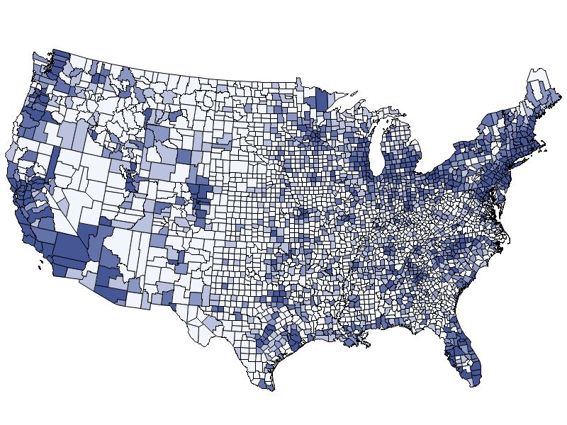
Figure 2 shows the geographic distribution of M&As in the manufacturing sector. Figure
2a shows the number of deals in each county from 1990 to 2014, while Figure 2b shows the total
transaction value (in 2010 dollars) in each county during the same period. The acquisitions in
the manufacturing sector show some geographic pattern in concentration. For example, most
of the deals are concentrated in the northeast as well as on the west coast, most likely because
8
Different states have different starting times on reporting to the QWI data. For example, Massachusetts did
not start reporting until 2010.
14of the geographic concentration of industries.
4. Effect of M&As on Employment Growth
4.1. Establishment Level Analysis
The first section of the empirical analysis focuses on the effect of M&As on the employment
at the target establishments. Following previous studies9 , I estimate the following matched
difference-in-differences design:
Log(Emp)i,t = β0 + β1 T reatedi × P ostt + θi + ωt + i,t , (11)
where Log(Emp)i,t is the log employment of establishment i at time t. treated is an indicator
that equal 1 if the establishment experienced an M&A. P ostt is the indicator for the peri-
ods after the M&A. The interaction between treated and post dummy captures the average
treatment effect of the M&A deal. θic] measures the year-fixed effects and ωi measures the es-
tablishment fixed effects. i,t is the error term. β1 is the main coefficient of interest. A negative
and statistically significant β1 implies that M&As have a negative impact on the employment
level at the target establishments. Standard errors are clustered at the establishment level.
Panel A of table 2 reports the results. In column (1) and (2), I focus on establishments from
all industries. In column (1), the T reated∗P ost term is negative and statistically significant. It
indicates that compared to the control establishments, the acquired establishments on average
experienced a greater decline in employment level. The coefficient of -0.013 indicates that
compared to the control establishments, the treated establishments on average experiences
a 1.3% decrease in employment after the merger. In column (2) of table 2, I weight the
regression by the number of employees during the year before the merger. The coefficient of the
9
Existing studies such as Li (2013), Ma et al. (2016), Lagaras (2018), etc. use similar approaches to test the
establishment level employment change after M&As
15T reated∗P ost term remains negative and statistically significant. The acquired establishment
on average experienced a 2.4% decline in employment level. In Column (3) and (4), I shift
the focus to establishments in the manufacturing sector and repeat the test. In both columns,
the coefficient of treated × post indicator is negative and statistically significant. Column 3
(column 4) shows that, compared with the control establishments, the treated establishments
are associated with a 1.5%(2.5%) decline in employment after the completion of M&As.
To test the dynamic timing of the employment change after M&A at the establishment
level, I modify equation (11) by interacting each time dummy with the treated dummy. Specif-
ically, I estimate the following regression
k=3
X
yi,j,t = β0 + βk T reated × D[t + k]i,j,t + θi + ωt + i,t (12)
k=−3
Where D[t+k]i,t are dummy variables for observations that are k years from the acquisition.
Panel B of Table 2 reports the estimation results. In all the four columns in panel B, there is
no statistically significant difference in employment level before the treated establishments and
control establishments before the acquisition. However, after the acquisition become effective,
the coefficient on the interactions demonstrate a monotonic change. Figure (3) presents the
coefficeint plots of column (2) and (4) in panel B.
4.2. MSA Level Analysis
My analysis on the spillover effect of M&As on the local labor market is based on the com-
parison between MSAs that experienced M&As at different times. In the baseline analysis, I
estimate the following MSA-quarter level panel regression:
Employment Growthi,t = β0 + β1 M &AEventi,t + β2 Xi,t + ηi + πt + i,t , (13)
16where Employment Growthi,t measures the three-year employment growth rate of M SAi .
I focus on the three-year employment growth rate because it takes time for employment
changes to take effect after an M&A. M &AEventi,t is an indicator that equals one if M SAi
experienced a significant jump in merger activities in the past four quarters10 . Xi,t denotes
a vector of time-varying demographic characteristics including four-quarter lagged MSA level
employment and four-quarter lagged total income. In the main model specifications, I also
control the share of employment in the manufacturing sector at time t-4 as MSAs with varying
degrees of dependency on the manufacturing sector might be affected differently by mergers
in the manufacturing sector. I include MSA and time fixed effects, which are denoted by ηi
and πt , respectively, to control for MSA-invariant and time-invariant variables.
4.3. Effect on Employment growth in the Manufacturing Sector
table 3 reports the results of the baseline regressions. The dependent variable is the three-
year employment growth rate in the manufacturing sector. In column (1), I control for the
MSA and year-quarter fixed effects. The coefficient -0.006 indicates that compared with the
MSAs without experiencing M&A Event in the past four quarters, an MSA that experienced
a significant jump in merger activities in the past 4 quarters is associated with a 2.2% lower
three-year employment growth rate in the next three years. This result is economically sig-
nificant compared to the unconditional mean of -2.0%. In column (2), I control for MSA
characteristics by including log (Total income) and log (Total labor force) as control vari-
ables, both of which are four-quarter lagged MSA level variables. The coefficient of the Deal
dummy remains negative and statistically significant. The coefficient decreases from 0.006
to 0.005 compared to column (1) but the magnitude remains economically large. In column
(3), I follow Autor et al. (2013) and control for the share of the manufacturing sector in the
previous year to address the possibility that the deal variable could, in part, be picking up
an overall declining trend in the U.S. manufacturing sector rather than being caused by a
10
The results estimated with windows from 1-3 quarters are consistent with the baseline findings.
17merger completion. The estimated coefficient indicates that an MSA with one percentage
point higher initial manufacturing share experiences a 1.38% lower employment growth rate
in the next three years.
Finally, in column (4), I introduce the state × quarter-fixed effect to address the possibility
of heterogeneous trends across states. Some states might experience specific transitions in
industry composition, so controlling the state × quarter-fixed effects can effectively address
the possible effect caused by state time-varying heterogeneity. The coefficient on the Deal
dummy remains statistically significant at -0.01, indicating that MSAs with target firms in
the past four quarters are associated with a one percentage point lower three-year employment
growth in the manufacturing sector.
Taken together, the results from columns (1) to (4) suggest that when a target firm in the
manufacturing sector is acquired, it causes a sector-wide employment slowdown in the MSA
where the target is located. Lagaras (2018) finds that M&As are associated with a significant
decline in employment in target firms through increased layoffs. My findings show that the
negative effect on employment growth can spread to the whole sector.
4.4. Effect on Employment Growth in the Non-Tradable Sector
The previous section has established the relation between mergers and acquisitions and the
decline in the employment growth rate in the manufacturing sector. In this section, I examine
the spill over of the negative effects on employment growth to the non-tradable sector. As
illustrated by Mian and Sufi (2014), the non-tradable sector, such as retail and restaurants,
depend heavily on local demand. Consequently, a layoff after the completion of an M&A is
expected to lower the average wages and consumer demand of the local community.
I follow Mian and Sufi (2014) and Adelino et al. (2017) to define the non-tradable sector
as consisting of Retail Trade (two-digit NAICS 44-45) and Accommodation and Food Services
(two-digit NAICS 72). I replace the dependent variable in the baseline regressions with the
18three-year employment growth rate in the non-tradable sector and repeat the regressions
specified in equation (1). table 4 shows the results.
In table 4, columns (1) to (4) repeat the tests as the same column numbers in table 3. In
column (1), the model with no control variables indicates that an MSA that has a target firm
in the manufacturing sector acquired in the past four quarters is expected to have a 0.3% lower
average three-year employment growth rate in the non-tradable sector than MSAs without an
M&A Event in the past four quarters. Further, in columns (2) and (3), where I control for
MSA characteristics, the economic magnitude of the coefficient on the Deal dummy decreases
slightly to 1%; however, this is still economically significant compared to the unconditional
sample mean of 4.3%. Finally, to address the issue that different states could have different
trends during the sample period, I repeat the same process as in Table 2 and control for state
by time-fixed effects. The coefficient on the Deal dummy drops to 60 basis points, indicating
that with the completion of a merger, the declined local demand contributes to a 60 basis
points lower three-year employment growth in the local area. I adopt column (4) in table 4
as the main model specification in the following tests.
A back-of-the-envelope calculation shows that, for an average MSA, a completed merger
is associated with about 290 more job losses in manufacturing sector in the next three years
while the declined employment growth is associated with 300 less job creations in the non-
tradable sector. Overall, the results in table 4 indicate that there is a “hidden” cost of M&As
that is borne by the local community where the target is located. By laying off redundant
workforce and improving corporate efficiency, M&As lead to a slower employment growth in
the local area, not only for the manufacturing sector where the target belongs, but also for
other sectors, such as the non-tradable sector.
194.5. Robustness Analysis
table 5 shows that M&As are associated with slower employment growth in the non-tradable
sector. In this section, I first address the concern that the above results might be driven
by other confounding factors by employing two placebo tests. First, I change the timing
of the completion of M&A deals by replacing the actual completion date with a placebo
completion date 12 quarters before the actual date. If acquirers pick up targets from areas
with deteriorating conditions in the manufacturing sector or the local economy, then it is the
deteriorating economic conditions, rather than the M&A, that causes the findings reported
in the previous sections. In this case, the false deal completion dates should show a similarly
negative effect on employment growth.
Column (1) of table 5 reports the results with the false completion dates. The dependent
variable is the three-year employment growth rate in the non-tradable sector. The coefficient
on the Deal dummy is neither statistically nor economically significant, indicating that it is
not the economic conditions associated with the local economy that drive the results reported
in the previous sections. Rather, it is the M&As that cause a slower employment growth in
the MSAs where the target firms are located.
Second, I follow Seru (2014) and Ma et al. (2016) to replace completed deals with with-
drawn deals as “placebos.” If the Deal variable simply picks up the trend of declining industry
or local area conditions, a similar effect should be expected for withdrawn deals. I repeat the
baseline regression with withdrawn deals in column (2) of table 5. As seen, the coefficient
on the Deal dummy is neither statistically or economically significant. Therefore, the merger
deals have to be completed to show the negative effect on employment growth. This suggests
that the corporate restructuring resulting from completed M&As trigger the spillover effect
to the non-tradable sector.
Third, as Figure 1 shows, a large fraction of the M&As in the manufacturing sector took
place around the Financial Crisis. The Crisis could affect local consumer demand by lowering
20household net wealth. To address this, I exclude the observations from 2007 to 2010 and
repeat the tests. The results on the non-tradable sector employment growth are similar after
the completion of the deal. Finally, I follow Autor et al. (2013) and estimate the exposure
of local area to Chinese import penetration. The effect of M&A Events remains similar after
controling for the potential effect of Chinese import penetration. Overall, the tests in table 5
confirm the findings from the baseline regressions that M&As in manufacturing sector have a
negative spillover effect on the local labor market in areas where the target firms are located.
4.6. 2SLS Analysis
The previous sections reveal that completion of mergers in the manufacturing sector has a
negative spillover effect on the non-tradable sector employment by lowering local consumer
demand. However, the correlation can hardly be interpreted as causal because unobserved
economic factors can drive both employment growth in the non-tradable sector and an M&A.
To address such an empirical challenge, I construct an instrument to capture the arguably
exogenous variation in the probability that an MSA has a M&A target. The literature connect-
ing stock market valuation with the probability of corporate takeover finds that undervalued
firms are more likely to be selected as targets in takeovers(Shleifer and Vishny, 2003; Edmans
et al., 2012). Similarly, if more firms from the same industry are undervalued, the industry
should be more likely to become a target industry. Hence, if an undervalued industry accounts
for a large fraction of the local employment, the area might be more appealing for potential
acquirers and be more likely to have M&A targets. Overall, this identification strategy hinges
on the notion that MSAs with different undervalued industries might have different ex-ante
probabilities to have M&A targets.
I identify the exogenous shocks in local valuation in the local area in the following way
X Empi,m
Sm,t = Discounti,t , (14)
i
Empm
21where Empi,m measures the employment of 4-digit NAICS manufacturing industry i of
MSA m when the MSA first enters into the sample. Empm measures the total employment
of MSA m when the MSA first enters the sample. I measure the local presence using the first
available observation of an MSA to mitigate the concern of potential feedback effects from
local labor market to stock valuation. I follow Edmans et al. (2012) and use Discounti,t as the
valuation measure. Discounti,t measures by how much the firms from industry i are traded
11
to their maximum potential value absent managerial inefficiency and mispricing.
The identification assumption in equation (12) is that while the probability of having a
merger target is likely to be endogenously related to local economic conditions, an indus-
try’s valuation is more likely to be driven by aggregate economic shocks. Areas with different
ex-ante exposure to each industry would experience different changes in local valuations. How-
ever, the local valuation measure Si,t is also subject to potential bias. As Edmans et al. (2012)
suggests, stock prices are endogenous and increase in anticipation of a takeover. Therefore, if
an industry is concentrated in one area, the idiosyncratic shock to the area (housing market
crash, disasters etc.) could affect industry valuation.
To address this, I calculate the weighted average discount (market value) for all firms in
L L
the same MSA Si,t . Then, I regress the original measure Si,t on Si,t and take the residual
L
term S̃i,t . If Si,t captures the common valuation shocks shared by all firms in the local area,
S̃i,t will be orthogonal to the local economic conditions and serve as a valid instrument to the
existence of targets in the MSA. I then estimate the following regression
M &A Eventm,t = α0 + α1 × S̃m,t−1 + α2 × Xm,t + m,t , (15)
where α1 is expected to be negative if areas with industries that have higher valuation are
11
Specifically, I follow Edmans et al. (2012) to construct the discount measure based on Tobin’s Q. The
successful firms in an industry are defined as firms that rank on the 80th percentile in their 4-digit NAICS
industry. I calculate the discount measure as (Q∗ − Q)/Q∗ . See Edmans et al. (2012) for more details. I
then aggregate the discount measure of each industry with the weight of total market cap.
22less likely to experience a merger. In the second stage, I estimate the following regression
¯
∆EM Pm,t,t+12 = β0 + β1 × M &A Eventm,t + β2 × Xm,t + m,t , (16)
¯
where M &A Eventm,t denotes the predicted probability of an M&A event in the local MSA.
Columns (1) and (2) of table 6 report the first stage regression. The local discount instrument
is negative and statistically significant on the probability that the MSA will experience an
M&A Event. A 1 SD increase in the local discount instrument is associated with a 2.2% lower
probability of an M&A Event. Considering that the unconditional mean of the M&A Event
is only about 5%, this effect is economically significant as well. The local discount instrument
has a strong explanatory power with partial F-statistics of 13.32 and 13.79 in columns 1 and 2,
respectively. In columns (3) and (4), I test the effect of merger completion on manufacturing
sector employment growth. The reduced form regression in column (3) indicates that a 1 SD
increase in the local discount instrument is associated with a 50 basis points increase in the
manufacturing sector employment. Additionally, column (4) suggests that a 1 SD increase
in the local discount instrument is associated with 70 basis points higher growth rate in the
employment of the non-tradable sector.
In the last four columns of table 6, I report the coefficient estimates for the second-stage
regression. All coefficients in columns (5) to (7) show negative and significant effects on
employment growth rate in the manufacturing and non-tradable sectors, consistent with the
ordinary least squares (OLS) results. Including or removing the control variables do not affect
the point estimates significantly. However, it is important to notice that the point estimates of
the instrumental variable (IV) regression are much higher than the point estimates in the OLS
regression. The greater IV effect indicates that takeovers driven by differences in valuation
lead to a greater drop in employment growth than average takeovers. This is possible as
the acquiring firms could identify undervalued targets and realize the potential value gain
through labor restructuring. Alternatively, the IV estimates could capture the marginal effect
of a large valuation change. Acquiring firms might only approach a target when the target is
23significantly undervalued. I use the OLS result as the preferred model because it shows the
average effect of M&As and is more conservative.
4.7. Wage and Migration Effects
In table 7, I analyze the effects of mergers in the manufacturing sector on the MSA’s wage
growth. I repeat the baseline regressions and replace the dependent variable with the three-
year average weekly wage growth rate. In column (1) of table 7, I study the change in wage
growth in the manufacturing sector. The Deal dummy is negatively correlated with the three-
year wage growth rate with a coefficient of -0.008, indicating that MSAs with completed
mergers are expected to experience an 80 basis points lower growth in wage in the manufac-
turing sector. This finding is consistent with the hypothesis that mergers are associated with a
higher probability of layoffs. Lower labor demand in the manufacturing sector might also lead
to lower wages. Next, I shift my focus to the wage growth in the non-tradable sector. Column
(2) of table 6 shows that the three-year wage growth in the non-tradable sector is statistically
significant at 10% with an economic magnitude of 40 basis points. This finding is consistent
with that of Mian and Sufi (2014), who find little evidence on wage change in the non-tradable
sector despite a decline in the non-tradable sector employment after the Financial Crisis. One
possible explanation here is that non-tradable sector could have low wage elasticity.
In columns (3) and (4) of table 7, I explore the effect of M&As on the migration of
workforce following a merger completion. According to Autor et al. (2013), a large mobility
response indicates that initial local impacts will rapidly diffuse across regions. Following
previous studies (Mian and Sufi, 2014), I use two different measures to test labor mobility
response after the completion of a merger12 . In column (3), I test the change in the three-
year population growth rate after the completion of a merger. The coefficient on the Deal
dummy is negative but statistically insignificant. In column (4), I test the change in the
12
Since the data on population is only available on an annual basis, the tests in columns (3) and (4) in table
7 are conducted at annual MSA level
24three-year labor force growth rate after the completion of a merger. In contrast to the results
on population growth, the three-year labor force growth rate is negatively and statistically
significantly associated with deal completion, indicating that although there are not many
people leaving the MSA, people are quitting the job market because of the weak demand
resulting from the merger deal. When combined, the results from columns (3) and (4) in table
7 further confirm the decline in local consumer demand after merger completion.
4.8. Household Level Analysis
The previous sections have established the relation between merger completion and the spillover
effects at the MSA level. In this section, I analyze how merger completion affects the local
labor market using the household-level data from SIPP. My purpose is to find evidence at the
micro level to corroborate the findings at the aggregate MSA level. I estimate the following
regression:
Outcomei,b,t = α0 + α1 × T reatedi × P ostb,t + α2 × T reatedi
+ α3 × P ostb,t + α4 × Xb,t + α5 × Yi,t + ηb + ωt + θi + i,t , (17)
where T reatedi is an indicator of whether the individual is working in the manufacturing
13
sector (the non-tradable sector) during the year before the merger completion. P ostb,t
is an indicator if MSA b experienced a completed merger at time (t-3, t). Xb is a vector
of the characteristics of MSA b at time t and Yi,t is a vector of individual characteristics of
individual i. ηb indicates the time-invariant MSA heterogeneity. ωt represents the year-fixed
effect and θi represents the individual-fixed effects. To study the effect of completed mergers
on the household, I focus on two outcomes. First, the probability that an individual stays
in the manufacturing sector (the non-tradable sector) and second, the probability that the
13
For MSAs without any completed mergers during the sample period, the treated dummy is defined based
on the sector of the individuals’ first appearance in the sample.
25individual loses his job.
table 8 reports the summary statistics of the household-level data. The individuals in
the sample have an average age of about 40 and 53% are married. About 10% of the sample
observations work in the manufacturing sector and about 12% work in the non-tradable sector.
14
Overall, about 73% of the individuals in the sample are employed during the sample period.
table 8 reports the estimated results.
In panel A of table 9, I test the effect of completion of M&As on individuals working in
the manufacturing sector. The treated dummy is defined as one if the individual works in the
manufacturing sector during the year before the merger completion. In columns (1) to (3),
the dependent variable is the probability that an individual works in the manufacturing factor
after the merger completion. In column (1), I do not include control variables; in column
(2), I control for all individual characteristics and MSA characteristics;15 and in column (3),
I control MSA× year-fixed effects to address the potential issue that different MSAs could
have different trends in the local labor market. The coefficient on the interaction term treated
× post is negative and statistically significant, indicating that an individual working in the
manufacturing sector before the completion of merger is more likely to leave the sector. The
estimated coefficient is equal to -0.045 across three model specifications, indicating that after
the merger completion, a treated individual is 4.5% less likely to remain in the manufacturing
sector. In columns (4) to (6), I test the probability that an individual remains employed after
the merger completion. The coefficient estimates in columns (4) to (6) indicate that individuals
who worked in the manufacturing sector before the completion of mergers are 3.2% to 3.7%
more likely to become unemployed during the three-year period after the merger.
Further, I test the effect of merger completion on workers in the non-tradable sector. The
treated dummy in panel B of table 9 is defined as one if an individual was working in the non-
14
The relative size of employment in the non-tradable and manufacturing sectors for the same period in the
QWI data is similar to that of the SIPP data.
15
The control variables include MSA population, average income, unemployment rate, household size, age,
college degree, and whether the individual is married.
26tradable sector during the year before the merger. Like the results of panel A, the coefficient
on treated×post is negative and statistically significant in all specifications, indicating that
individuals working in the non-tradable sector are more likely to leave the sector after merger
completion. The effect is also economically significant. In columns (1) to (3) of panel B,
a treated individual is about 7% more likely to leave the non-tradable sector after merger
completion. Further, as columns (4) to (6) indicate, an individual working in the non-tradable
sector is 3% more likely to become unemployed after merger completion. Overall, the results
from table 9 confirm the findings at the MSA level that M&As in the manufacturing sector
not only lead to a reduction in employment in the manufacturing sector, but also lead to a
negative spillover on employment in the non-tradable sector.
4.9. Cross-sectional Variation
4.9.1. Firm Heterogeneity
I further explore the heterogeneous impact of M&As on the employment growth for firms of
different ages. I follow Appel et al. (2019) and aggregate the QWI data for young firms (less
than or equal to 5 years old), mature firms (6-10 years old), and old firms (older than 10 years)
and calculate the three-year employment growth rate separately for each group. Columns (1)
to (3) in table 9 report the estimated results for the firms in different age groups, indicating
that young and old firms are more likely to be affected, while the effect is trivial on mature
firms. Column (1) in table 10 shows that an MSA with a completed merger is associated
with a 90 basis points lower three-year employment growth rate among young firms in the
non-tradable sector. These results are consistent with that of Adelino et al. (2017) that young
firms from the non-tradable sector account for the bulk of net employment creation in response
to local demand shocks. Similarly, firms that are more than 10 years old are also subject to
the negative impact of merger completion although the economic magnitude is smaller (50
basis points).
27You can also read