Ensemble flood simulation for a small dam catchment in Japan using nonhydrostatic model rainfalls - Part 2: Flood forecasting using 1600-member ...
←
→
Page content transcription
If your browser does not render page correctly, please read the page content below
Nat. Hazards Earth Syst. Sci., 20, 755–770, 2020
https://doi.org/10.5194/nhess-20-755-2020
© Author(s) 2020. This work is distributed under
the Creative Commons Attribution 4.0 License.

Ensemble flood simulation for a small dam catchment in Japan
using nonhydrostatic model rainfalls – Part 2: Flood forecasting
using 1600-member 4D-EnVar-predicted rainfalls
Kenichiro Kobayashi1 , Le Duc1,2,6 , Apip1,3 , Tsutao Oizumi2,6 , and Kazuo Saito4,5,6
1 Research Center for Urban Safety and Security, Kobe University, 1-1 Rokkodai-machi, Nada-ku, Kobe, 657-8501, Japan
2 Japan Agency for Marine-Earth Science and Technology (JAMSTEC), Yokohama, Japan
3 Research Centre for Limnology, Indonesian Institute of Sciences (LIPI), Bogor, Indonesia
4 Japan Meteorological Business Support Center, Tokyo, Japan
5 Atmosphere and Ocean Research Institute, the University of Tokyo, Kashiwa, Japan
6 Meteorological Research Institute, Tsukuba, Japan

Correspondence: Kenichiro Kobayashi (kkobayashi@phoenix.kobe-u.ac.jp)

Received: 13 November 2018 – Discussion started: 9 January 2019
Revised: 25 November 2019 – Accepted: 4 February 2020 – Published: 23 March 2020

Abstract. This paper is a continuation of the authors’ pre-        1   Introduction
vious paper (Part 1) on the feasibility of ensemble flood
forecasting for a small dam catchment (Kasahori dam; ap-
prox. 70 km2 ) in Niigata, Japan, using a distributed rainfall–    Flood simulation driven by ensemble rainfalls has attracted
runoff model and rainfall ensemble forecasts. The ensem-           more attention in recent years, resulting in a lot of use-
ble forecasts were given by an advanced four-dimensional,          ful information that ensemble flood forecasts can provide in
variational-ensemble assimilation system using the Japan           flood control, such as forecast uncertainty, probabilities of
Meteorological Agency nonhydrostatic model (4D-EnVar-              rare events and potential flooding scenarios. In the Japanese
NHM). A noteworthy feature of this system was the use of           case, it is considered that the ensemble rainfall simulation
a very large number of ensemble members (1600), which              with a high resolution (2 km or below) is desirable, since ex-
yielded a significant improvement in the rainfall forecast         treme rainfall often takes place due to mesoscale convective
compared to Part 1. The ensemble flood forecasting using the       systems and the river catchments are not as large as con-
1600 rainfalls succeeded in indicating the necessity of emer-      tinental rivers; even the largest Tone River basin is around
gency flood operation with the occurrence probability and          17 000 km2 .
enough lead time (e.g., 12 h) with regard to an extreme event.        A good review of ensemble flood forecasting using
A new method for dynamical selection of the best ensemble          medium-term global and European ensemble weather fore-
member based on the Bayesian reasoning with different eval-        casts (2–15 d ahead) by numerical weather prediction (NWP)
uation periods is proposed. As the result, it is recognized that   models can be found in Cloke and Pappenberger (2009).
the selection based on Nash–Sutcliffe efficiency (NSE) does        In much of their review, the resolution of NWP model is
not provide an exact discharge forecast with several hours         relatively coarse (over 10 km), the number of ensembles is
lead time, but it can provide some trend in the near future.       moderate (10–50) and the target catchment size is often
                                                                   large (e.g., Danube River Basin). They basically reviewed
                                                                   global and European ensemble prediction systems (EPSs)
                                                                   but also introduced some research on regional EPSs nested
                                                                   into global EPSs (e.g., Marsigli et al., 2001). They stated
                                                                   that “One of the biggest challenges therefore in improving
                                                                   weather forecasts remain to increase the resolution and iden-

Published by Copernicus Publications on behalf of the European Geosciences Union.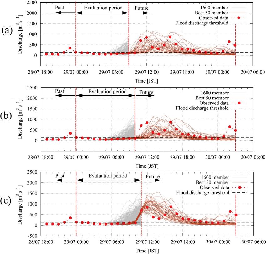
756                          K. Kobayashi et al.: Ensemble flood simulation for a small dam catchment in Japan – Part 2

tify the adequate physical representations on the respective      event. Their ensemble weather simulation model resolution
scale, but this is a source hungry task”.                         was 2.5 km by AROME from Météo-France, which uses AL-
   Short-term flood forecasting (1–3 d) based on ensemble         ADIN forecasts for lateral boundary conditions (10 km res-
NWPs is gaining more attention in Japan. Kobayashi et             olution); thus the deep convection was explicitly resolved.
al. (2016) dealt with an ensemble flood (rainfall–runoff) sim-    We can recognize from this research that the European re-
ulation of a heavy-rainfall event that occurred in 2011 over a    searchers especially around mountain regions have been far-
small dam catchment (Kasahori dam; approx. 70 km2 ) in Ni-        sighted from early days for the importance of these cloud-
igata, central Japan, using a rainfall–runoff model with a res-   resolving ensemble simulations.
olution of 250 m. Eleven-member ensemble rainfalls by the            On the other hand, in Japan, Yu et al. (2018) have also
Japan Meteorological Agency nonhydrostatic model (JMA-            used a post-processing method using the spatial shift of NWP
NHM; Saito et al., 2006) with horizontal resolutions of 2 and     rainfall fields for correcting the misplaced rain distribution.
10 km were employed. The results showed that, although            Their study areas are the Futatsuno (356.1 km2 ) and Nanairo
the 2 km EPS reproduced the observed rainfall much bet-           (182.1 km2 ) dam catchments of the Shingu river basin, lo-
ter than the 10 km EPS, the resultant cumulative and hourly       cated on the Kii Peninsula, Japan. The resolutions of the
maximum rainfalls still underestimated the observed rainfall.     ensemble weather simulations were 10 and 2 km by JMA-
Thus, the ensemble flood simulations with the 2 km rainfalls      NHM, which is similar to the downscaling EPS in Kobayashi
were still not sufficiently valid, and a positional lag correc-   et al. (2016) but for a different heavy-rainfall event in western
tion of the rainfall fields was applied. Using this translation   central Japan caused by a typhoon. The results showed that
method, the magnitude of the ensemble rainfalls and likewise      the ensemble forecasts produced better results than the de-
the inflows to the Kasahori dam became comparable with the        terministic control run forecast, although the peak discharge
observed inflows.                                                 was underestimated. Thus, they also carried out a spatial shift
   Other applications of the 2 km EPS, which permit deep          of the ensemble rainfall field. The results showed that the
convection on some level, can be found in studies, for ex-        flood forecasting with the spatial shift of the ensemble rain-
ample that of Xuan et al. (2009). They carried out an en-         fall members was better than the original one; likewise the
semble flood forecasting at the Brue catchment, with an area      peak discharges more closely approached the observations.
of 135 km2 , in southwestern England, UK. The resolution of          Recently, as a further improvement upon the 2 km down-
their grid-based distributed rainfall–runoff model (GBDM)         scale ensemble rainfall simulations used by Kobayashi et
was 500 m, and the resolution of their NWP forecast by the        al. (2016), Duc and Saito (2017) developed an advanced
PSU/NCAR (Pennsylvania State University–National Cen-             data assimilation system with the ensemble variational
ter for Atmospheric Research) mesoscale model (MM5) was           method (EnVar) and increased the number of ensemble
2 km. The NWP forecast was the result of downscaling of           members to 1600. This new data assimilation system was
the global forecast datasets from the European Centre for         aimed to improve the rainfall forecasts of the 2011 Niigata–
Medium-Range Weather Forecasts (ECMWF). Fifty mem-                Fukushima heavy-rainfall event (JMA, 2013; Niigata Prefec-
bers of the ECMWF EPS and one deterministic forecast were         ture, 2011). The torrential rain of this event occurred over the
downscaled. Since the original NWP rainfall of a grid av-         small area along the synoptic-scale stationary front (for sur-
erage still underestimates the intensity compared with rain       face weather map, see Fig. 1 of Kobayashi et al., 2016). Saito
gauges, they introduced a best-match approach (location cor-      et al. (2013) found that the location where intense rain con-
rection) and a bias-correction approach (scale-up) on the         centrates varied in small changes of the model setting; thus
downscaled rainfall field. The results showed that the en-        the position of the heavy rain was likely controlled by hori-
semble flood forecasting of some rainfall events is in good       zontal convergence along the front rather than the orographic
agreement with observations within the confidence intervals,      forcing.
while that of other rainfall events failed to capture the basic      Since the new EPS produced better forecasts of the rainfall
flow patterns.                                                    fields, in this study, Part 2 of Kobayashi et al. (2016), we ap-
   Likewise in Europe, Hohenegger et al. (2008) carried out       plied those 1600-member ensemble rainfalls to the ensemble
the cloud-resolving ensemble weather simulations of the Au-       inflow simulations of Kasahori dam. In this series, consist-
gust 2005 Alpine flood. Their cloud-resolving EPS of 2.2 km       ing of Part 1 and 2, we intentionally chose a rainfall–runoff
grid space included the explicit treatment of deep convec-        model whose specification is quite close to those runoff mod-
tion and was the result of downscaling of COSMO-LEPS              els used in many governmental practices of Japanese flood
(10 km resolution driven by ECMWF EPS). Their conclu-             forecasting to see the usefulness of 1600-member ensemble
sion was that despite the overall small differences, the 2.2 km   rainfalls. Our objective is to assess impact of the improve-
cloud-resolving ensemble produces results as good as and          ment of the rainfall forecast over the large area around Kasa-
even better than its 10 km EPS, though the paper did not deal     hori dam on the streamflow forecast for the Kasahori dam. In
with the hydrological forecasting. Another paper which dealt      Part 1 the technique of positional lag correction was applied
with cloud-resolving ensemble simulations can be found in         to match the rainfall forecasts with the observations to have a
Vie et al. (2011) for a Mediterranean heavy-precipitation         better hydrological forecast. This technique is hard to apply

Nat. Hazards Earth Syst. Sci., 20, 755–770, 2020                           www.nat-hazards-earth-syst-sci.net/20/755/2020/
K. Kobayashi et al.: Ensemble flood simulation for a small dam catchment in Japan – Part 2 757
in real-time flood forecasting, since rainfall observations are lation system using the Japan Meteorological Agency non-
unknown and there are a lot of potential positional lag vectors hydrostatic model (4D-EnVar-NHM) was newly developed
to choose from. Statistically the positional lag vector should in which background error covariances were estimated from
respond to the local orographic features, but it may vary de- short-range ensemble forecasts by JMA-NHM before being
pending on the synoptic condition on the day and model fore- plugged into functions for minimization to obtain the analy-
cast errors in a specific event. Thus the positional lag vector ses (Duc and Saito, 2017). If the number of ensemble mem-
for one extreme rainfall event basically cannot be applied to bers is limited, ensemble error covariances contain sampling
other extreme event as is. The new EPS is expected to remove noises which manifest as spurious correlations between dis-
the use of such a technique. tant grid points. In data assimilation, the so-called localiza-
In addition, the very large number of ensemble members, tion technique is usually applied to remove such noise, but
which is 10 to 20 times larger than the typical number of at the same time it removes significant correlations in er-
ensemble members currently run in operational forecast cen- ror covariances. In this study, we chose 1600 members in
ters, poses new issues needed to solve in computation and running the ensemble part of 4D-EnVar-NHM to retain sig-
interpretation. First, regional forecast centers may not af- nificant vertical correlations, which have a large impact on
ford running 1600 hydrological forecasts in real time, and a heavy-rainfall events like the Niigata–Fukushima heavy rain-
method to choose the most important members may be help- fall. That means only horizontal localization is applied in
ful. Such a method is known as ensemble reduction in en- 4D-EnVar-NHM. The horizontal localization length scales
semble forecasts (Molteni et al., 2001; Montani et al., 2011; were derived from the climatologically horizontal correla-
Hacker et al., 2011; Weidle et al., 2013; Serafin et al., 2019), tion length scales of the JMA’s operational four-dimensional,
which is built upon cluster analysis when observations are variational assimilation system JNoVA by dilation using a
not used as guidance for selection. However, our problem is factor of 2.0.
more interesting when we can access the observations in the Another special aspect of 4D-EnVar-NHM is that a sepa-
first few hours, and ensemble reduction should make use of rate ensemble Kalman filter was not needed to produce the
these past observations in selecting important members. Sec- analysis ensemble. Instead, a cost function was derived for
ond, it is more challenging to interpret the result when tem- each analysis perturbation, and minimization was then ap-
poral and spatial uncertainties are realized to be more distinct plied to obtain this perturbation, which is very similar to the
now. Without taking such uncertainties into account, the en- case of analyses. This helped to ensure consistency between
semble forecasts are easily to be considered useless. analyses and analysis perturbations in 4D-EnVar-NHM when
The organization of this paper is as follows. Section 2 de- the same background error covariance, the same localization
scribes the new mesoscale EPS and its forecast and rainfall and the same observations were used in both cases. To accel-
verification results. Section 3 describes the rainfall–runoff erate the running time, all analysis perturbations were calcu-
model for explaining the changes in the model parameters. lated simultaneously using the block algorithm to solve the
Results are shown in Sect. 4. In Sect. 5, concluding remarks linear equations with multiple right-hand-side vectors result-
and future aspects are presented. ing from all minimization problems. The assimilation system
was started at 09:00 JST on 24 July 2011 with a 3 h assimi-
lation cycle. All routine observations at the JMA’s database
2 Mesoscale ensemble forecast were assimilated into 4D-EnVar-NHM. The assimilation do-
main was the same as the former operational system at the
2.1 Ensemble prediction system JMA. To reduce the computational cost, a dual-resolution ap-
proach was adopted in 4D-EnVar-NHM where analyses had
An advanced mesoscale EPS was developed and employed a grid spacing of 5 km, whereas analysis perturbations had
to prepare precipitation data for the rainfall–runoff model. a grid spacing of 15 km. The analysis and analysis perturba-
The EPS was built around the operational mesoscale model tions were interpolated to the grid of the ensemble prediction
JMA-NHM for its atmospheric model as the downscale EPS system to make the initial conditions for deterministic and
conducted by Saito et al. (2013). In this study, a domain con- ensemble forecasts.
sisting of 819 × 715 horizontal grid points and 60 vertical
levels was used for all ensemble members. This domain had 2.2 Rainfall verification
a grid spacing of 2 km and covered the mainland of Japan.
With this high resolution, convective parameterization was Due to limited computational resources, ensemble forecasts
switched off. Boundary conditions were obtained from fore- with 1600 members were only employed for the target time
casts of the JMA’s global model. Boundary perturbations of 00:00 JST on 29 July 2011. However, deterministic fore-
were interpolated from forecast perturbations of the JMA’s casts were run for all other initial times to examine the impact
operational 1-week EPS as in Saito et al. (2013). of the number of ensemble members on analyses and the re-
To provide initial conditions and initial perturbations for sulting forecasts. Figure 1 shows the verification results for
the EPS, a four-dimensional, variational-ensemble assimi- the 3 h precipitation forecasts as measured by the fraction
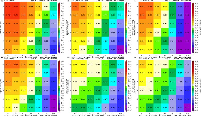
www.nat-hazards-earth-syst-sci.net/20/755/2020/ Nat. Hazards Earth Syst. Sci., 20, 755–770, 2020758 K. Kobayashi et al.: Ensemble flood simulation for a small dam catchment in Japan – Part 2 Figure 1. Fraction skill scores of 3 h precipitation at Niigata–Fukushima from deterministic forecasts initialized by analyses from JNoVA (a, b) and 4D-EnVar-NHM using 1600 (c, d) and 50 members (e, f). These scores are averaged over the period from 21:00 JST on 24 July to 21:00 JST on 29 July 2011. To obtain robust statistics, precipitation is aggregated over the first 12 h forecasts (valid between 3 and 12 h forecast) and the next 12 h forecasts (valid between 12 and 24 h forecasts) as shown in the top and bottom rows, respectively. Note that the first 3 h precipitation is discarded due to the spin-up problem. skill score (FSS; Roberts and Lean, 2008). Given a rainfall 4DEnVar50 to differentiate it from the original one, 4DEn- threshold and an area around a grid point, which is called a Var1600, was run. The main difference between 4DEnVar50 neighborhood, the FSS measures the relative difference be- and 4DEnVar1600 is that vertical localization was applied tween observed and forecasted rainfall fractions in this area. in the former case to generate its ensemble members. As This verification score is used to mitigate difficulty in rainfall mentioned in the previous section, vertical localization can verification at the grid scale with very high resolution fore- potentially weaken vertical flows in convective areas by re- casts in which high variability in rain fields usually makes moving physically vertical correlations. It is very clear from the traditional scores inadequate due to their requirement of Fig. 1 that 4DEnVar1600 outperforms 4DEnVar50 almost for an exact match between observations and forecasts at grid all precipitation thresholds, especially for intense rain. Also points. Thus the solution that the FSS follows is to consider for the high rain rate, compared to JNoVA, 4DEnVar1600 forecast quality at spatial scales coarser than the grid scale forecasts are worse than JNoVA forecasts for the first 12 h by comparing forecasts and observations not at grid points forecasts, which can be attributed to the fact that 4D-EnVar- but at neighborhoods whose sizes are identified with spatial NHM did not assimilate satellite radiances and surface pre- scales. The FSS is normalized to range from 0 to 1, with the cipitation like JNoVA. However, it is interesting to see that value of 1 indicating a perfect forecast and the value of 0 be- 4D-EnVar-NHM produces forecasts better than JNoVA for ing a no-skill forecast which can be obtained by a random very intense rain for the next 12 h forecasts. forecast. To check the reliability of the ensemble forecasts, reliabil- In Fig. 1 we aggregate the 3 h precipitation in the first and ity diagrams are calculated and plotted in Fig. 2 for 4DEn- second 12 h forecasts to increase samples in calculating the Var1600 and 4DEnVar50. Since JNoVA only provided de- FSS. In this way, robust statistics are obtained, but at the terministic forecasts, the reliability diagram is irrelevant for same time dependence of the FSS on the leading times can JNoVA. Note that we only performed ensemble forecasts still be shown. Note that an additional experiment with 4D- initialized at the target time of 00:00 JST on 29 July 2001 EnVar-NHM using 50 ensemble members, which is called due to lack of computational resource to run 1600-member Nat. Hazards Earth Syst. Sci., 20, 755–770, 2020 www.nat-hazards-earth-syst-sci.net/20/755/2020/
K. Kobayashi et al.: Ensemble flood simulation for a small dam catchment in Japan – Part 2                                                759

Figure 2. As in Fig. 1 but for reliability diagrams of 3 h precipitation from ensemble forecasts initialized by analysis ensembles of 4D-EnVar-
NHM using 1600 and 50 members. Three precipitation thresholds of 1 mm (a, b), 10 mm (c, d) and 50 mm (e, f) are chosen. Note that the
ensemble forecasts were only run for the time 00:00 JST on 29 July 2011.

ensemble forecasts at different initial times. Therefore, the                As examples of the forecasts, Fig. 3 shows the accumu-
same strategy of aggregating 3 h precipitation over the first             lated precipitation at the peak period (12:00–15:00 JST on
and second 12 h forecasts in calculating the FSS in Fig. 1 is             29 July 2011) as observed and forecasted by the 4D-EnVar
applied to obtain significant statistics. Clearly, Fig. 2 shows           prediction system. Here, the rainfall observations were ob-
that 4DEnVar1600 is distinctively more reliable than 4DEn-                tained from the operational precipitation analysis system of
Var50 in predicting intense rain. While 4DEnVar50 cannot                  JMA based on radar and rain-gauge observations, which is
capture intense rain, 4DEnVar1600 tends to overestimate ar-               called the radar–AMeDAS (RA) – Automated Meteorologi-
eas of intense rain. The tendency of overestimation of 4DEn-              cal Data Acquisition System. For comparison, the determin-
Var1600 becomes clearer if we consider the forecast ranges                istic forecast initialized by the analysis from JNoVA using
between 12 and 24 h. However, for the first 12 h, 4DEn-                   the same domain was also given. Note that the forecast range
Var1600 slightly underestimates areas of light rains. This                corresponding to this peak period is from 12 to 15 h. Clearly,
also explains why the FSSs of 4DEnVar1600 are smaller than                the deterministic forecast initialized by 4D-EnVar-NHM out-
those of 4DEnVar50 for small rainfall thresholds in Fig. 1.               performed that by the JNoVA, especially in terms of the lo-
                                                                          cation of the heavy rain, although the forecast by 4D-EnVar-

www.nat-hazards-earth-syst-sci.net/20/755/2020/                                     Nat. Hazards Earth Syst. Sci., 20, 755–770, 2020
760 K. Kobayashi et al.: Ensemble flood simulation for a small dam catchment in Japan – Part 2
NHM tended to slightly overestimate the rainfall amount, as Table 1. The equivalent roughness coefficient of the forest, the
verified by the reliability diagrams in Fig. 2. This overestima- Manning coefficient of the river, and identified soil-related parame-
tion can also be observed in the coastal area near the Sea of ters of Part 2 (this paper) and Part 1 (Kobayashi et al., 2016).
Japan. Note that a significant improvement was also attained
against the former downscale EPS used in Part 1 (see Fig. 9 Forest River D Ks
(m−1/3 s−1 ) (m−1/3 s−1 ) (m) (m s−1 )
of Kobayashi et al., 2016).
Since it is not possible to examine all 1600 forecasts, the This paper (RA) 0.424 0.010 0.522 0.0010
ensemble mean forecast is only plotted in Fig. 3d. Again, the This paper (RC) 0.170 0.005 0.234 0.0008
Part 1 0.150 0.004 0.320 0.0005
location of the heavy rain corresponds well with the observed
location, as in the case of the deterministic forecast, but the
ensemble mean precipitation is smeared out as a side effect
of the averaging procedure. Therefore, the ensemble mean RA and RC and observations are shown in Fig. 5 with a
should not be used in our hydrological model as a represen- RA hyetograph. The duration of the calibration simulation
tative of the ensemble forecast. Instead, all ensemble precip- is from 01:00 JST on 28 July to 00:00 JST on 31 July 2011.
itation forecasts should be fed into the hydrological model to The Nash–Sutcliffe efficiency (hereinafter NSE: Nash and
avoid rainfall distortion caused by averaging in addition to Sutcliffe, 1970), which is used for the assessment of model
a faithful description of rainfall uncertainty. Of course with performance, is calculated as follows:
1600 members this causes a huge increase in computational N
2
Qio − Qis
P
cost, and we try to reduce this burden by testing a suitable dy-
i=1
namical selection, described later in Sect. 4. To have a glance NSE = 1 − , (1)
N
to the performance of the ensemble forecast we plot 1 h ac- 2
Qio − Qm
P
cumulated precipitation over the Kasahori dam catchment in i=1
time series in Fig. 4 (observed data are radar–AMeDAS). It N
1 X
can be seen that while the deterministic forecast could some- Qm = Qi , (2)
how reproduce the three-peak curve of the observed rainfall, N i=1 o
ensemble members tended to capture the first peak only. Note
where N is the total number of time steps (1 h interval), Qio is
that some members showed this three-peak curve, such as
observed dam inflow (discharge) at time i, Qis is simulated
the best member, but their number was much lower than the
dam inflow (discharge) at time i, and Qm is the average of
number of ensemble members.
the observed dam inflows.
In the calibration simulations in Fig. 5, the NSEs with RA
and RC are 0.686 and 0.743, respectively. Although the NSE
3 Distributed rainfall–runoff (DRR) model with RA is worse than RC, the total rainfall amount with RA
is considered more accurate, and the second and third dis-
The DRR model used in Part 1 was applied again in this
charge peaks seem to be captured better with RA; thus the
paper. See Kobayashi et al. (2016) for the details. The
following discussion will be made basically with the pa-
DRR model applied was originally developed by Kojima et
rameters calibrated with RA. Some results with RC will be
al. (2007) and called CDRMV3. As described in the previ-
added as references. The main difference of the parameters
ous section, we intentionally chose a rainfall–runoff model
between RA and RC is that the surface soil thickness D to
whose specification is close to those runoff models used by
hold the rainfall at the initial stage is thicker in RA, which
national and local governments, since the purpose is more
yields the lower discharge in the river.
to investigate the usefulness of 1600-member ensemble rain-
falls.
The parameters of the DRR model were recalibrated in this 4 Results
study using hourly radar–AMeDAS, since the amount of to-
tal rainfall for the period (762.8 mm) is closer to ground rain In this section, the results of the ensemble flood simulations
gauge (765.0 mm; Kobayashi et. al., 2016). The hourly radar are shown, focusing on two aspects:
composite (RC; radar data) of JMA was also used for another
1. We examined whether the ensemble inflow simulations
recalibration as a reference, since radar precipitation data
can show the necessity of the flood control operation
are in general the primary source for real-time flood fore-
and emergency operation with the probability and suffi-
casting. The total rainfall amount with RC was 568.5 mm,
cient lead time (e.g. 12 h).
which is smaller than the ground rain gauge (765.0 mm).
The recalibrated equivalent roughness coefficients of the for- 2. We also examined if we could obtain high accuracy en-
est, the Manning coefficients of the river and the identified semble inflow predictions several hours (1–3 h) before
soil-related parameters are described in Table 1 with the pa- the occurrence, which could contribute to the decision
rameters in Part 1. The simulated discharge hydrographs by for optimal dam operation.
Nat. Hazards Earth Syst. Sci., 20, 755–770, 2020 www.nat-hazards-earth-syst-sci.net/20/755/2020/K. Kobayashi et al.: Ensemble flood simulation for a small dam catchment in Japan – Part 2 761 Figure 3. Three-hour accumulated precipitation from 12:00 to 15:00 JST on 29 July 2011 at Niigata–Fukushima as observed by radar– AMeDAS (RA) (a), forecasted by NHM initialized by the analysis of JNoVA (b), forecasted by NHM initialized by the analysis of 4D- EnVar-NHM (c) and forecasted by the ensemble mean forecast of NHM initialized by the analysis ensemble of 4D-EnVar-NHM (d). All forecasts were started at 00:00 JST on 29 July 2011. Figure 4. Time series of 1 h accumulated rainfall over the catchment as forecasted by all ensemble members. The observation, control forecast, ensemble mean forecast and best member forecast are also plotted for comparison. Here, the best member is defined as the member that has the minimum distance between its time series and the observed time series. www.nat-hazards-earth-syst-sci.net/20/755/2020/ Nat. Hazards Earth Syst. Sci., 20, 755–770, 2020
762                          K. Kobayashi et al.: Ensemble flood simulation for a small dam catchment in Japan – Part 2

Figure 5. RA hyetograph, observed dam inflow, and simulated inflows with RA and RC.

Item (1) provides us with the scenario that we can prepare for      range unlike the 1600 ensembles; thus 50 ensemble dis-
any dam operations with enough lead time. Likewise, it may          charges cannot be used for the forecasting as they are.
enable us to initiate early evacuation of the inhabitant living        Figure 7 shows the probability that the inflow discharge is
downstream of the dam. Item (2) is the target that has been         beyond 140 m3 s−1 (hereinafter expressed as q > 140, where
attempted by researchers of flood forecasting. If we could          q is the discharge), the threshold value for starting the flood
forecast the inflow almost correctly several hours before the       control operations. The figure considers the temporal shift of
occurrence, it could help the dam administrator with the de-        the ensemble rainfalls, i.e., temporal uncertainty due to the
cision for actual optimal dam operations.                           imperfect rainfall simulation. In the figure, 0 h uncertainty
                                                                    means that we only considered discharges at time t to cal-
4.1   Probabilistic forecast                                        culate probability, while the 1 h uncertainty means that we
                                                                    considered the discharges at t − 1, t, t + 1, to calculate prob-
Item (1) is considered first herein. Figure 6 shows the com-        ability, and the 2 h uncertainty means that we considered the
parisons of the hydrographs of (a) 11 discharge simula-             discharges at t − 2, t − 1, t, t + 1, t + 2, to calculate prob-
tions in Part 1, (b) the same 11 members but with a posi-           ability. The 3 and 4 h uncertainties were calculated in the
tional shift in Part 1, (c) 50 discharge simulations with 4D-       same way. It becomes clear from the figure that the starting
EnVar-NHM and parameters by RA, (d) 1600 discharge sim-             time of q > 140 is likely at around t = 10:00 JST on 29 July,
ulations with 4D-EnVar-NHM and parameters by RA, and                where all curves cross, while the ending time is likely at
(e) 1600 discharge simulations with 4D-EnVar-NHM and pa-            t = 19:00 JST, where all curves cross again. Before and after
rameters by RC. Note that the duration of the 4D-EnVar-             the cross points there are jumps in the probabilities. In other
NHM ensemble weather simulation is 30 h from 00:00 JST              words, the forecast can indicate that the situation of q > 140
on 29 July 2011 to 07:00 JST on 30 July 2011, but the en-           would take place after 10 h from the beginning of forecasting
semble flood simulation is carried out only for 24 h from           with the probability of around 50 %.
03:00 JST on 29 July 2011 to 03:00 JST on 30 July 2011,                On the other hand, the emergency operation was under-
since we consider that JMA-NHM uses the first 3 h to ad-            taken in the actual flood event. In the emergency operation,
just its dynamics. The result in Fig. 6d and e shows that, ex-      the dam outflow has to equal the inflow to avoid dam fail-
cept for the third peak, the 1600-member ensemble inflows           ure as the water level approaches the top of the dam body.
can encompass the observed discharge within the 95 % confi-         As written in Part 1, when the reservoir water level reaches
dence bound, which was not realized in Part 1, with 11 down-        EL 206.6 m (EL – elevation level), an emergency operation is
scale ensemble rainfalls of 2 km resolution (Fig. 6a). In other     undertaken, and the outflow is set to equal the inflow. As the
words, the extreme rainfall intensity of the event can be re-       height–volume (H–V) relationship of the dam reservoir was
produced by the ensemble members with 1600 4D-EnVar-                not known during the study, we judged the necessity of the
NHM on some level. By comparing (d) with (e), it is recog-          emergency operation by whether the cumulative dam inflow
nized that the 95 % confidence and interquartile bound of (d)       was beyond the flood control capacity of 8 700 000 m3 . Actu-
is narrower than (e); thus the prediction with the parameters       ally, the flood control capacity had not been previously filled
calibrated with RA, a physically more accurate rainfall, can        during regular operations more than the estimation given
reduce the uncertainty of the prediction probably because of        herein, since the dam can release the dam water by natural
the better physical meaning in the parameters. It is consid-        regulation. However, again, since we do not know some of
ered also that the ensemble mean and median values capture          the relationships to calculate the dam water level, the judg-
the overall trend of the observations on some level.                ment is made based on whether the cumulative dam inflow
   Likewise, comparing Fig. 6c and d, we can recognize that         exceeds the flood control capacity.
the simulated discharges by 50 ensemble rainfalls of 4D-               Figure 8 shows the cumulative dam inflows of all the en-
EnVar-NHM do not encompass the observation within the               semble simulations starting from 03:00 JST on 29 July 2011

Nat. Hazards Earth Syst. Sci., 20, 755–770, 2020                             www.nat-hazards-earth-syst-sci.net/20/755/2020/
K. Kobayashi et al.: Ensemble flood simulation for a small dam catchment in Japan – Part 2 763 Figure 6. Hydrographs of (a) 11 discharge simulations in Part 1 (Kobayashi et al., 2016), (b) the same 11 members but with a positional shift in Part 1, (c) 50 discharge simulations with 4D-EnVar-NHM and model parameters by RA, (d) 1600 discharge simulations with 4D-EnVar- NHM and model parameters by RA, and (e) 1600 discharge simulations with 4D-EnVar-NHM and model parameters by RC. www.nat-hazards-earth-syst-sci.net/20/755/2020/ Nat. Hazards Earth Syst. Sci., 20, 755–770, 2020
764 K. Kobayashi et al.: Ensemble flood simulation for a small dam catchment in Japan – Part 2
Figure 7. Probability that the simulated inflow is beyond 140 m3 s−1 considering temporal uncertainty.
as well as the 95 % confidence and interquartile bound and will be used up with the probability of more than 90 % with
the mean, median and observed cumulative inflow with the regard to this flood event.
flood control capacity – (a) with parameters by RA and
(b) with parameters by RC. Figure 8a shows that the mean of 4.2 Selection of the best members
the cumulative dam inflows underestimates the observation,
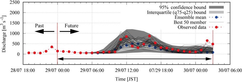
while in Fig. 8b the mean was roughly similar to the observa- Figure 10 shows the 95 % confidence interval of all ensem-
tion. Thus, it is considered that many of the 1600-member en- ble members, the 50 best ensemble members out of 1600 en-
semble rainfalls still underestimate the total rainfall amount sembles selected based on NSE > 0.33 and observations. The
compared with RA rainfall, though the observed cumulative figure shows that the selected 50 members reproduce the ob-
dam inflow is covered within the 95 % confidence interval of servations well. In some of the selected members, even the
the ensemble inflows with RA parameters. As a reference, third peak is reproduced. In the case where the third peak is
Fig. 8b shows that if the hydrological model parameters are reproduced, the inflow hydrographs are beyond the 95 % con-
calibrated with less rainfall (this case RC), underestimated fidence interval. Figure 11 shows the catchment average rain-
ensemble rainfalls yield higher discharges, which resulted in falls of the 50 best ensemble inflow simulations. The black
an almost equivalent mean of the ensembles compared with line is the observed gauge rainfall, the blue line is the radar–
the observation, though this is considered to be a bias cor- AMeDAS and the green line is the radar composite, while
rection from the hydrological model (see also Fig. 6d and e the grey lines are the 50 rainfalls for the best ensemble dis-
for the comparison). Figure 9 shows the probability that the charges. The rainfalls from the best 50 ensemble inflow sim-
cumulative dam inflow exceeds the flood control capacity ulations resemble those of the radar–AMeDAS.
of 8 700 000 m3 . The figure indicates that, for instance, the Clearly, the flood forecasting becomes very useful if we
cumulative inflow would exceed flood control capacity af- could just select the best ensemble members in advance. Log-
ter 12 h from the start of the forecast with the probability ically, this is impossible, since we only know the best mem-
of around 15 % (RA parameters) and 45 % (RC parameters). bers after knowing the observations which enable us to com-
In the actual event, the cumulative inflow based on obser- pute verification scores like the NSE. This raises the question
vations, and assuming no dam water release, would exceed of whether or not the best ensemble members can be inferred
the flood control capacity between 12:00 and 13:00 JST on from the partial information provided by the observations in
29 July 2011. Around that interval, the exceedance probabil- the first few hours. It is easy to see that the answer should be
ity of the forecast is 15 %–30 % (RA parameters) and 35 %– negative due to nonlinearity of the model and the presence
55 % (RC parameters). Until around this time, the forecast of model error: the best matching in the first few hours is al-
shows a delay in the estimate of the cumulative dam inflow. most certainly not the best matching over all forecast ranges.
In the end, the forecast shows that the flood control capacity However, it is obvious that the observations at the first few
hours have a certain value which can help to reduce uncer-
Nat. Hazards Earth Syst. Sci., 20, 755–770, 2020 www.nat-hazards-earth-syst-sci.net/20/755/2020/K. Kobayashi et al.: Ensemble flood simulation for a small dam catchment in Japan – Part 2 765 Figure 8. Cumulative dam inflow by the ensemble simulations, mean of simulation and observations, and critical dam volume (a) with parameters by RA and (b) with parameters by RC. Figure 9. Probability that the dam needs emergency operation. Radar–AMeDAS and radar composite indicate the ensemble simulation with the parameters calibrated with the rainfalls. www.nat-hazards-earth-syst-sci.net/20/755/2020/ Nat. Hazards Earth Syst. Sci., 20, 755–770, 2020
766                          K. Kobayashi et al.: Ensemble flood simulation for a small dam catchment in Japan – Part 2

Figure 10. Hydrographs of all 1600 ensemble members, the 50 best ensemble members (NSE > 0.33) and observations.

Figure 11. Rainfall intensity of the 50 best ensemble inflow simulation members, of radar–AMeDAS, of radar composite and of ground
observations.

                                                                     pre
tainty in the ensemble forecast if we could incorporate this       wi      denoting the equal weight for the ith member:
information into the forecast.
   This procedure has already been well-known under the                        K                                 K
                                                                               X       pre
                                                                                                                X   1
name “data assimilation”, in which we assimilate the obser-        pX (x) =           wi δ (x − x i ) =               δ (x − x i ) .                (3)
                                                                               i=1                              i=1
                                                                                                                    K
vations at the first few hours to turn the prior probabilistic
density function (pdf) given by the short-range forecasts into     Using this prior pdf as the proposal density, the posterior pdf
the posterior pdf given by the analysis ensemble (Kalnay,          has the following form:
2003; Reich and Cotter, 2015; Fletcher, 2017). Thus, if we
know the observations at the first few hours, we should as-                     K                               K
                                                                                X       post
                                                                                                                X               pY (y|x i )
                                                                   pX (x|y) =         wi       δ (x − x i ) =                                      . (4)
similate these data to replace the short-range ensemble fore-                                                         K
                                                                                i=1                             i=1
                                                                                                                      P
casts by the ensemble analyses at these hours, then run the                                                                  pY y|x j δ (x − x i )
                                                                                                                      j =1
model initialized by the new ensemble to issue a new ensem-
ble forecast. As a result, we should replace the definition of     Here, pY (y|x i ) denotes the likelihood of the observations y
                                                                                                                     post
the best members based on verification scores by a more ap-        conditioned on the forecast x i , and the weight wi is the rel-
propriate one based on the posterior pdf. Here, we identify        ative likelihood. Moreover, it can be shown that pY (y|x i ) is
the best members with the most likely members. Clearly, if         the observation evidence for the ith member (Duc and Saito,
we assume that the posterior pdf is unimodal, the best mem-        2018). Then applying the model M as the transition model,
bers should be the members clustering around the mode of           the predictive pdf is given by
this pdf, which is also the analysis. However, it is not clear
how to identify the best members if this pdf is multimodal.                            K
                                                                                                  post
                                                                                       X
   To overcome this problem, we will use the mathemati-            pX (x|y, M) =               wi        δ (x − M (x i )) .                         (5)
                                                                                        i=1
cal framework set up by particle filter (Doucet et al., 2001;
Tachikawa et al., 2011). Let us denote the short-range fore-       This equation shows that the contribution of each member
casts by x 1 to x K , where K is the number of ensemble mem-       to the predictive pdf is unequal, which differs from the prior
bers. The short-range ensemble forecast therefore yields an                                                                  post
                                             pre
                                                                   pdf (Eq. 3). While the members with large values of wi
empirical pdf given by the sample (x i , wi = 1/K), with           dominate the predictive pdf, those with very small values
                                                                        post
                                                                   of wi can be ignored. This suggests that the best members

Nat. Hazards Earth Syst. Sci., 20, 755–770, 2020                              www.nat-hazards-earth-syst-sci.net/20/755/2020/
K. Kobayashi et al.: Ensemble flood simulation for a small dam catchment in Japan – Part 2 767
post
can be identified with the largest values of wi . Thus, if we It is very clear from Fig. 12 that the set of the best mem-
post bers varies considerably with the time intervals of avail-
sort wi in the descending order, the first N weights corre-
spond to the first N best ensemble members. In this case, the able observations. This is because the NSE index is sensitive
predictive pdf (Eq. 5) is approximated by to the large difference between forecasts and observations.
This means that unless we simulate all the discharges of the
N 1600 members in advance, we may need to run many new
X pY (y|x i )
pX (x|y, M) = . (6) members to update this set every time when new observations
N
i=1
P
pY y|x j δ (x − M (x i )) are available, and this makes management of the best mem-
j =1 bers more complicated. To see why this occurs, suppose that
N−1
{Qio −Qis }2 are almost
P
Note that by introducing the notion of the best ensemble we have a member where the sums
members, a substantial change occurs – that is we now work i=1
post zero for the first 1, 2, . . . , N − 1 hours when we have no rain
with a unequal weighted sample (x i , wi ). This should be
or only light rain during this time. When we consider the next
taken into account in computing statistics like the ensemble N 2
hour to reselect the best members, if the term {QN o − Qs }
mean from the best ensemble members.
becomes very large, this member will suddenly be out of fa-
If the likelihoods have the Gaussian form
vor despite the fact that it is always selected as one of the best
members in all previous selection rounds. However, this large
1
pY (y|x i ) ∝ exp − (y − h (x i ))T R−1 (y − h (x i )) , (7) difference may come from spatial and temporal displacement
2
errors of rainfall forecasts and not necessary reflect an inac-
where h is the observation operator, and R is the observa- curate forecast. This shows that the use of the NSE in select-
tion error covariance, it is easy to see that the largest weights ing the best members is quite sensitive to spatial and tempo-
are corresponding to the smallest weighted root-mean-square ral displacement errors of rainfall. Part 1 of this study is an
errors (WRMSEs): illustration for impact of spatial displacement errors on fore-
cast performance, while Figs. 7 and 9 here show the case of
WRMSEi = (y − h (x i ))T R−1 (y − h (x i )) . (8) temporal displacement errors. On the other hand, the NSE of
rainfall cannot be used to select the best discharge members,
Therefore, if R is a multiple of the identity matrix I, the since rainfall NSEs of similar values can produce different
WRMSEs become the RMSEs, which in turn are equivalent discharge hydrographs. For example, the catchment average
to the NSEs. This shows that selection of the best members rainfall with an NSE of around 0 produces discharges with
based on verification scores over the first few hours is in fact an NSE close to 0.5 and −0.5. The spatial distribution of the
selection of the best members based on the relative likeli- rainfall field causes these differences even though the num-
hoods in the posterior pdf. It can also be understood as model ber of the catchment average rainfalls is the same. Even if
selection based on observation evidence (Mackay, 2003). the catchment area is small, different patterns in the rain-
To check the work of this method of dynamical selec- fall field bring different discharge simulations with different
tion, we attempted to select some of the best members out NSEs. Furthermore, the error model for rainfall does not fol-
of the 1600 members several hours in advance of the event low the Gaussian distribution, and a more appropriate dis-
based only on NSEs for the discharges. Figure 12a shows tribution like a gamma or log-normal distribution should be
a result where we selected the best 50 ensemble members used. However, such distributions make NSEs irrelevant, and
(NSE > 0.24) for the first 9 h from the start of the forecast. In new verification scores derived from these distributions are
this case, we had a 3 h lead time towards the observed peak needed, which can take a form that is like the FSS. Thus,
discharge, and the selected 50 members cover the observed it is expected that if we can introduce spatial and temporal
discharge after the first 9 h on some level. The result shows uncertainty in modeling the likelihood pY (y|x i ), the predic-
that the ensemble inflow simulations selected can indicate tive pdf (Eq. 6) could yield a more useful ensemble forecast.
the possibility of rapid increases in the discharge after the However, this requires a lengthy mathematical treatment that
first 9 h with a 3 h lead time. is worth exploring in detail in a separate study.
Likewise Fig. 12b shows the selected best 50 members
(NSE > −0.04) for the first 10 h (2 h ahead of the observed
peak discharge). It is apparent that the result is worse than the 5 Concluding remarks and future aspects
previous first 9 h selection. The ensemble inflow simulations
after 10 h do not cover the observation well in this case. Fig- The study used 1600-member ensemble rainfalls produced
ure 12c shows the selected best 50 members (NSE > 0.92) by 4D-EnVar which contain various rainfall fields with dif-
for the first 11 h (1 h ahead of the observed peak discharge). ferent rainfall intensities. No post-processing such as the lo-
In this case, the ensemble inflows after 11 h could cover the cation correction of the rainfall field and/or rescaling of rain-
observed peak discharge 1 h later on some level, although it fall intensity was employed. The ensemble flood forecast us-
only has a 1 h lead time. ing the 1600-member ensemble rainfalls in this study has
www.nat-hazards-earth-syst-sci.net/20/755/2020/ Nat. Hazards Earth Syst. Sci., 20, 755–770, 2020768 K. Kobayashi et al.: Ensemble flood simulation for a small dam catchment in Japan – Part 2 Figure 12. (a) Best 50 ensemble members (NSE > 0.24) selected from first 9 h forecast, (b) best 50 ensemble members (NSE > −0.04) selected from first 10 h forecast and (c) best 50 ensemble members (NSE > 0.92) selected from first 11 h forecast. shown that the extremely high amount of observed inflow the Xth hour. In other word, we cannot select the best dis- discharge can be reproduced within the confidence interval, charge simulation from the NSE only until X hours. Herein which was not possible by the 11-member downscale ensem- lies the problem that NSEs are quite sensitive to spatial and ble rainfalls used in Part 1. The NSE of the best member out temporal displacement errors in rainfall. In principle, it is of 1600 was 0.72. Likewise, we can calculate the probability possible to introduce those errors into NSEs in a way similar of occurrence (e.g. the necessity of emergency dam opera- to FSSs. However, it should be cautious in introducing such tions) with the 1600-member ensemble rainfalls. Thus, the errors into NSEs before investigating well, although such an result of the study shows that the ensemble flood forecasting approach has been used recently in the meteorology commu- can inform us that, after 12 h for example, emergency dam nity. How to incorporate them qualitatively is also a problem operations would be required with the probability of around to be addressed. Thus, in this sense, the dynamical selection 15 %–30 %, the probability would be more than 90 % for the of the best rainfall field from rainfall simulations considering entire flood event, etc. We consider that this kind of infor- both spatial and temporal displacement errors is required, al- mation is very useful. For instance, a warning of dam water though this was not addressed here and remains for future release can be issued to the inhabitant in the downstream with work. enough lead time if the result obtained in this study is further applicable to other locations and events. On the other hand, the discharge simulations with similar Data availability. JMA-NHM is available under the collabora- NSEs until X hours produce different future forecasts after tive framework between the Meteorological Research Institute Nat. Hazards Earth Syst. Sci., 20, 755–770, 2020 www.nat-hazards-earth-syst-sci.net/20/755/2020/
K. Kobayashi et al.: Ensemble flood simulation for a small dam catchment in Japan – Part 2                                                 769

(MRI) and related institutes or universities. Likewise, the DRR         Doucet, A., de Freitas, N., and Gordon, N. J.: Sequential Monte
model is available under the collaborative framework between               Carlo Methods in Practice, Springer-Verlag, New York, USA,
Kobe and Kyoto universities and related institutes or universi-            2001.
ties. The JMA’s operational analyses and forecasts can be pur-          Duc, L. and Saito, K.: A 4DEnVAR data assimilation system with-
chased at http://www.jmbsc.or.jp/jp/online/file/f-online10200.html         out vertical localization using the K computer, in: Japan Geo-
(last access: 11 March 2020) (JMA, 2019). Likewise, radar                  science Union meeting, 20–25 May 2017, Chiba, Japan, AAS12-
composite analyses and radar rain-gauge analyses can be pur-               P04, 2017.
chased at http://www.jmbsc.or.jp/jp/online/file/f-online30100.html      Duc, L. and Saito, K.: Verification in the presence of observation
(last access: 11 March 2020) and http://www.jmbsc.or.jp/jp/online/         errors: Bayesian point of view, Q. J. Roy. Meteorol. Soc., 144,
file/f-online30400.html (last access: 11 March 2020), respectively         1063–1090, https://doi.org/10.1002/qj.3275, 2018.
(JMA, 2019). The rain-gauge data and hydrological data were pro-        Fletcher, S. J.: Data Assimilation for the Geosciences: From Theory
vided by MLIT (personal communication, 2011), the Niigata Pre-             to Application, Elsevier, Amsterdam, the Netherlands, 2017.
fecture (personal communication, 2011) or JMA at http://www.data.       Hacker, J. P., Ha, S. Y., Snyder, C., Berner, J., Eckel, F. A., Kuchera,
jma.go.jp/gmd/risk/obsdl/index.php (last access: 11 March 2020)            E., Pochernich, M., Rugg, S., Schramm, J., and Wang, X.: The
(JMA, 2013). We will consider making other data available upon             US Air Force Weather Agency’s mesoscale ensemble: scien-
request. Research cooperation is preferable for the data provision.        tific description and performance results, Tellus A, 63, 625–641,
                                                                           https://doi.org/10.1111/j.1600-0870.2010.00497.x, 2011.
                                                                        Hohenegger, C., Walser, A., Langhans, W., and Schaer, C.:
Author contributions. KK managed all research activity of the pa-          Cloud-resolving ensemble simulations of the August 2005
per except the 1600-member ensemble meteorological simulations.            Alpine flood, Q. J. Roy. Meteorol. Soc., 134, 889–904,
Likewise, KK contributed to a large part of the paper preparation.         https://doi.org/10.1002/qj.252, 2008.
LD managed the research work of the meteorological part, includ-        JMA – Japan Meteorological Agency: Report on “the 2011 Niigata-
ing the 1600-member ensemble meteorological simulations. LD                Fukushima heavy rainfall event”, typhoon Talas (1112) and
also contributed to a large part of the paper preparation. A carried       typhoon Roke (1115), Tech. Rep. JMA, available at: http://
out the 1600 rainfall–runoff simulations. TO engaged in the figure         www.jma.go.jp/jma/kishou/books/gizyutu/134/ALL.pdf (last ac-
preparation and data analysis. KS provided advice on the overall           cess: 11 March 2020), 2013.
research activity, especially focusing on the meteorological aspects.   JMA – Japan Meteorological Agency: Outline of the op-
                                                                           erational numerical weather prediction at the Japan
                                                                           Meteorological Agency, Tech. Rep. JMA, available
Competing interests. The authors declare that they have no conflict        at:          https://www.jma.go.jp/jma/jma-eng/jma-center/nwp/
of interest.                                                               outline2019-nwp/pdf/outline2019_all.pdf            (last      access:
                                                                           11 March 2020), 2019.
                                                                        Kalnay, E.: Atmospheric modeling, data assimilation and pre-
                                                                           dictability, Cambridge Univ. Press, London, UK, 2003.
Acknowledgements. Computational results were obtained using the
                                                                        Kobayashi, K., Otsuka, S., Apip, and Saito, K.: Ensemble flood
K computer at the RIKEN Advanced Institute for Computational
                                                                           simulation for a small dam catchment in Japan using 10 and
Science.
                                                                           2 km resolution nonhydrostatic model rainfalls, Nat. Hazards
                                                                           Earth Syst. Sci., 16, 1821–1839, https://doi.org/10.5194/nhess-
                                                                           16-1821-2016, 2016.
Financial support. This work was supported by the Ministry of           Kojima, T., Takara, K., and Tachikawa, Y.: A distributed runoff
Education, Culture, Sports, Science and Technology as Field                model for flood prediction in ungauged basin, Predictions in
3, the Strategic Programs for Innovative Research (SPIRE) and              ungauged basins: PUB kick off, IAHS Publ., Oxfordshire, UK,
the FLAGSHIP 2020 project (Advancement of meteorological                   267–274, 2007.
and global environmental predictions utilizing observational “Big       Mackay, D. J. C.: Information theory, inference, and learning Algo-
Data”). Project IDs are as follows: hp140220, hp150214, hp160229,          rithms, Cambridge Univ. Press, London, UK, 2003.
hp170246, hp180194 and hp190156.                                        Marsigli, C., Montani, A., Nerozzi, F., Paccagnella, T., Tibaldi,
                                                                           S., Molteni, F., and Buizza, R.: A strategy for high–resolution
                                                                           ensemble prediction. Part II: limited-area experiments in four
Review statement. This paper was edited by Kai Schröter and re-            alpine flood events, Q. J. Roy. Meteorol. Soc., 127, 2095–2115,
viewed by Alan Seed and two anonymous referees.                            https://doi.org/10.1002/qj.49712757613, 2001.
                                                                        Molteni, F., Buizza, R., Marsigli, C., Montani, A., Nerozzi, F.,
                                                                           and Paccagnella, T.: A strategy for high-resolution ensemble
                                                                           prediction. I: Definition of representative members and global-
                                                                           model experiments, Q. J. Roy. Meteorol. Soc., 127, 2069–2094,
                                                                           https://doi.org/10.1002/qj.49712757612, 2001.
References                                                              Montani, A., Cesari, D., Marsigli, C., and Paccagnella, T.: Seven
                                                                           years of activity in the field of mesoscale ensemble forecasting by
Cloke, H. L. and Pappenberger, F.: Ensemble flood                          the COSMO-LEPS system: main achievements and open chal-
  forecasting: A review, J. Hydrol., 375, 613–626,
  https://doi.org/10.1016/j.jhydrol.2009.06.005, 2009.

www.nat-hazards-earth-syst-sci.net/20/755/2020/                                    Nat. Hazards Earth Syst. Sci., 20, 755–770, 2020
770 K. Kobayashi et al.: Ensemble flood simulation for a small dam catchment in Japan – Part 2 lenges, Tellus A, 63, 605–624, https://doi.org/10.1111/j.1600- Tachikawa, Y., Sudo, M, Shiiba, M., Yorozu, K., and Sunmin, K.: 0870.2010.00499.x, 2011. Development of a real time river stage forecasting method using Nash, J. E. and Sutcliffe, V.: River flow forecasting through con- a particle filter, Journal of Japan Society of Civil Engineers, Ser. ceptual models part I – A discussion of principles, J. Hydrol., 10, B1, 67, I_511–I_516, https://doi.org/10.2208/jscejhe.67.I_511, 282–290, https://doi.org/10.1016/0022-1694(70)90255-6, 1970. 2011. Niigata Prefecture: Niigata/Fukushima extreme rainfall disaster Vie, B., Nuissier, O., and Ducrocq, V.: Cloud-resolving survey documentation (as of 22 August 2011), available at: ensemble simulations of Mediterranean heavy predic- http://www.pref.niigata.lg.jp/kasenkanri/1317679266491.html tion events: Uncertainty on Initial conditions and lateral (last access: 11 March 2020), 2011. boundary conditions, Mon. Weather Rev., 239, 403–423, Reich, S. and Cotter, C.: Probabilistic Forecasting and Bayesian https://doi.org/10.1175/2010MWR3487.1, 2011. Data Assimilation, Cambridge Univ. Press, UK, 2015. Weidle, F., Wang, Y., Tian, W., and Wang, T.: Validation Roberts, N. M. and Lean H. W.: Scale-selective verifica- of strategies using clustering analysis of ECMWF EPS tion of rainfall accumulations from high-resolution fore- for initial perturbations in a limited area model en- casts of convective events, Mon. Weather Rev., 136, 78–97, semble prediction system, Atmos.-Ocean, 51, 284–295, https://doi.org/10.1175/2007MWR2123.1, 2008. https://doi.org/10.1080/07055900.2013.802217, 2013. Saito, K., Fujita, T., Yamada, Y., Ishida, J., Kumagai, Y., Aranami, Xuan, Y., Cluckie, I. D., and Wang, Y.: Uncertainty analysis of K., Ohmori, S., Nagasawa, R., Kumagai, S., Muroi, C., Katao, hydrological ensemble forecasts in a distributed model utilizing T., Eito, H., and Yamazaki, Y.: The operational JMA nonhydro- short-range rainfall prediction, Hydrol. Earth Syst. Sci., 13, 293– static meso-scale model, Mon. Weather Rev., 134, 1266–1298, 303, https://doi.org/10.5194/hess-13-293-2009, 2009. https://doi.org/10.1175/MWR3120.1, 2006. Yu, W., Nakakita, E., Kim, S., and Yamaguchi, K.: Assessment of Saito, K., Origuchi, S., Duc, L., and Kobayashi, K.: Mesoscale ensemble flood forecasting with numerical weather prediction by ensemble forecast experiment of the 2011 Niigata-Fukushima considering spatial shift of rainfall fields, KSCE J. Civ. Eng., 22, heavy rainfall, Technical Report of the Japan Meteorolog- 3686–3696, https://doi.org/10.1007/s12205-018-0407-x, 2018. ical Agency, 170–184, available at: http://www.jma.go.jp/ jma/kishou/books/gizyutu/134/ALL.pdf (last access: 12 Febru- ary 2020), 2013. Serafin, S, Strauss, L., and Dorninger, M.: Ensemble reduction us- ing cluster analysis, Q. J. Roy. Meteorol. Soc., 145, 659–674, https://doi.org/10.1002/qj.3458, 2019. Nat. Hazards Earth Syst. Sci., 20, 755–770, 2020 www.nat-hazards-earth-syst-sci.net/20/755/2020/
You can also read