Why Australia was not wet during spring 2020 despite La Niña
←
→
Page content transcription
If your browser does not render page correctly, please read the page content below
www.nature.com/scientificreports
OPEN Why Australia was not wet
during spring 2020 despite La Niña
Eun‑Pa Lim1*, Debra Hudson1, Matthew C. Wheeler1, Andrew G. Marshall1, Andrew King2,
Hongyan Zhu1, Harry H. Hendon1,3, Catherine de Burgh‑Day1, Blair Trewin1,
Morwenna Griffiths1, Avijeet Ramchurn1 & Griffith Young1
The austral spring climate of 2020 was characterised by the occurrence of La Niña, which is the most
predictable climate driver of Australian springtime rainfall. Consistent with this La Niña, the Bureau
of Meteorology’s dynamical sub-seasonal to seasonal forecast system, ACCESS-S1, made highly
confident predictions of wetter-than-normal conditions over central and eastern Australia for spring
when initialised in July 2020 and thereafter. However, many areas of Australia received near average
to severely below average rainfall, particularly during November. Possible causes of the deviation
of rainfall from its historical response to La Niña and causes of the forecast error are explored with
observational and reanalysis data for the period 1979–2020 and real-time forecasts of ACCESS-S1
initialised in July to November 2020. Several compounding factors were identified as key contributors
to the drier-than-anticipated spring conditions. Although the ocean surface to the north of Australia
was warmer than normal, which would have acted to promote rainfall over northern Australia, it was
not as warm as expected from its historical relationship with La Niña and its long-term warming trend.
Moreover, a negative phase of the Indian Ocean Dipole mode, which typically acts to increase spring
rainfall in southern Australia, decayed earlier than normal in October. Finally, the Madden–Julian
Oscillation activity over the equatorial Indian Ocean acted to suppress rainfall across northern and
eastern Australia during November. While ACCESS-S1 accurately predicted the strength of La Niña
over the Niño3.4 region, it over-predicted the ocean warming to the north of Australia and under-
predicted the strength of the November MJO event, leading to an over-prediction of the Australian
spring rainfall and especially the November-mean rainfall.
Australian climate is the most predictable in springtime when large-scale oceanic and atmospheric circulations
typically exhibit large swings—the El Niño-Southern Oscillation (ENSO) is usually in its growth phase1,2; the
Indian Ocean Dipole (IOD) anomalies typically peak1,3 with or without a relation to ENSO4,5; the Antarctic
stratospheric polar vortex (SPV) anomaly usually peaks6–8; and the Southern Annular Mode (SAM)9,10 is strongly
influenced by ENSO and the Antarctic SPV8,11,12. These climate drivers play important roles in promoting climate
anomalies over different parts of Australia4,13, overall providing enhanced predictability across northern and
eastern Australia compared to the long-term mean behaviour (i.e., climatological forecast) or persistence from
the preceding conditions.
The 2019 spring to early summer climate was a good example of high predictability of Australian climate:
the IOD was near-record positive and was complemented by a central Pacific El Niño event, the Antarctic SPV
weakened dramatically becoming the near-weakest on record, and the October-December mean SAM was the
most negative on record for that season in the last 40 y ears14,15. Consequently, many regions of Australia during
spring and early summer 2019 experienced record hot and dry conditions especially over the Murray-Darling
basin and along the east coast15,16, which promoted severe bushfires that caused loss of lives and properties15,17.
The Bureau of Meteorology’s dynamical sub-seasonal to seasonal forecast system, ACCESS-S1 (Australian Com-
munity Climate Earth System Simulator-Seasonal version 1)18, skilfully predicted the large-scale conditions and
their impacts on Australia a season in advance14,15,19 (http://www.bom.gov.au/climate/ahead/outlooks/archive/
20190815-outlook.shtml), which was consistent with its well-documented ability to simulate and predict many
aspects of Australia’s weather and climate during spring and early s ummer20–24.
In contrast, spring 2020 showed much reduced prediction skill for Australia. From mid-2020 onwards La
Niña and the negative phase of the IOD were predicted by international forecast models (e.g., https://iri.colum
bia.edu/our-expertise/climate/forecasts/enso/2020-June-quick-look/?enso_tab=enso-sst_table), and a positive
1
Bureau of Meteorology, Melbourne, VIC, Australia. 2School of Geography, Earth, and Atmospheric Sciences and
ARC Centre of Excellence for Climate Extremes, University of Melbourne, Parkville, VIC, Australia. 3School of Earth
Atmosphere and Environment, Monash University, Clayton, VIC, Australia. *email: eun-pa.lim@bom.gov.au
Scientific Reports | (2021) 11:18423 | https://doi.org/10.1038/s41598-021-97690-w 1
Vol.:(0123456789)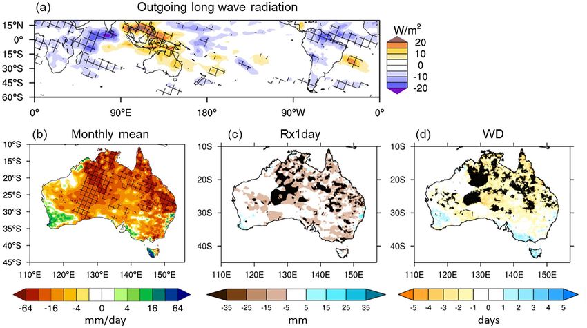
www.nature.com/scientificreports/
phase of the SAM was also anticipated during austral spring partly due to its relationship with La Niña11,25,26. As
La Niña, negative IOD and positive SAM are usually associated with springtime wet conditions over different
regions of Australia13,27, a much-wetter than normal spring was predicted by ACCESS-S1 with high confidence.
Both forecasts for La Niña and the positive SAM were verified well, the latter being partly thanks to an extra
forcing from the sudden stratospheric polar vortex strengthening during October–November (Fig. 1 and Sup-
plementary Fig. S1a). The negative IOD reached its maximum strength in August (−0.7 standard deviation (σ)
anomaly) but then rapidly decayed in October (Fig. 1c).
With these large-scale drivers at play, some parts of Australia received above-average spring rainfall, such as
South Australia and northwest Western Australia, but it was markedly less than expected from the emphatically
wet forecast, and there was significantly below average rainfall over south-eastern Queensland and north-eastern
New South Wales (Fig. 2). This forecast error over eastern Australia was an unpleasant surprise to the users of
seasonal forecasts, damaging the credibility of seasonal climate forecasts. In this study we review the large-scale
climate features of austral spring 2020 and investigate possible causes of the deviation of rainfall from its histori-
cal response to La Niña and causes of the forecast failure.
For the observational analyses over the period 1979–2020 we used: Reynolds OI v2 sea surface temperature
(SST) data28 for 1982–2020 and Hurrell et al.29 SST data for 1979–1981; NOAA interpolated outgoing longwave
radiation (OLR) d ata30; Japanese 55-year Reanalysis (JRA-55) d
ata31 for the global analysis of atmospheric vari-
ables; and the Australian Water Availability Project (AWAP) monthly mean rainfall data over Australia32. For
the forecast analyses we assessed the ACCESS-S1 forecasts initialised in July to November. For each variable,
the observed and forecast climatologies and standard deviations were computed for the period 1990–2012,
over which ACCESS-S1 hindcasts are available. Details of statistical analysis methods and ACCESS-S1 system
configurations are provided in “Methods”.
Large‑scale climate features and Australian rainfall in spring 2020
SSTs over the Niño 3.4 region (blue box in the tropical Pacific in Fig. 1a) started cooling from mid-2020 and
reached minus 1σ anomaly in September 2020 (Fig. 1c). This La Niña developed a central Pacific-flavour with the
maximum cold SST anomaly shifting westwards as the season progressed, which is evidenced by amplification
of the negative El Niño Modoki Index (EMI)33 while the Niño 3.4 SST cold anomaly weakened after October
(Fig. 1c). The strength of La Niña of austral spring 2020 was −1.2σ, which was comparable to that of 1998, 1999
and 2007, but weaker than that of 2010 (−1.6 σ) and 1988 (−1.9 σ) as judged by the Niño 3.4 September to
November mean SST anomaly.
The local SSTs surrounding Australia were significantly higher than normal, which we attribute to the occur-
rence of La Niña during the second half of 2020 and the long-term warming trend, which is statistically significant
at the 5% l evel34,35. Hendon et al.13 demonstrated that northern Australian rainfall in spring significantly increases
with higher SSTs north of Australia, which is monitored by an index of the SSTs averaged over the equator-10°S
and 110–160°E (SSTnAU; long-dashed black box in Fig. 1a). In austral spring 2020, SSTnAU was about 1σ higher
than normal, but this was substantially less than what was expected from the occurrence of the 2020 La Niña
and the long-term warming trend of the SSTnAU based on the historical relationships over 1979–2019. Based
on these relationships, the expected 2020 value was 2σ above normal, which would have been the warmest on
record since 1979 (Supplementary Fig. S2).
The IOD rapidly transitioned from being strongly positive in June (1.6σ), with higher-than-normal SST
over its western pole and lower-than-normal SST over its eastern pole (red and blue boxes in Fig. 1a), to being
moderately negative (−0.7σ) in August. The negative IOD did not last through austral spring but decayed in
October (Fig. 1c). Consequently, the springtime mean IOD amplitude was only −0.3σ. A more pronounced
feature over the tropical Indian Ocean was anomalous warming in the central part of the basin, which perhaps
was contributed to by the long-term upward t rend34,35. Over the period of 1979–2019, there has been a positive
trend in the IOD index (Dipole Mode Index; DMI), statistically significant at the 10% level in s pring36,37. Once
the linear trend was removed, the springtime mean IOD amplitude was -0.7σ, which implies that the long-term
warming trend in the tropical Indian Ocean acted to weaken the temperature difference between the east and
west poles of the negative IOD in spring 2020.
The SAM was in its positive phase, exhibiting moderate strength in October-December (Fig. 1c). However, the
near-surface circulation anomalies during spring 2020 did not follow a canonical zonally symmetric meridional
dipole pattern that has a mid-latitude zonal wavenumber-3 feature e mbedded11. Instead, its zonal symmetry was
disrupted by an equivalent barotropic Rossby wave train emerging from the tropical Indian Ocean, leading to the
zonal wavenumber-1 pattern in the SH high latitudes (Fig. 1b). This wave pattern highlights that the anomalous
tropical central Indian Ocean warming mentioned above is likely to have exerted strong forcing on the circula-
tion over the Southern Indian Ocean. The promotion of the positive SAM in late spring of 2020 could partly
be attributed to La Niña26, but is probably more closely related to the downward coupling from the near-record
strengthening of the Antarctic stratospheric polar vortex that occurred in October and November 2020, which
developed in conjunction with an extraordinary lack of upward propagation of planetary-scale waves from the
troposphere during spring 2020 (https://ozonewatch.gsfc.nasa.gov/meteorology/figures/merra2/heat_flux/vt1-
3w45_75-45s_100_2021_merra2.pdf) (Supplementary Fig. S3).
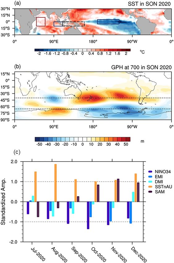
A regression analysis (Fig. 3 and Supplementary Figs. S4, S5) of the historical relationship of Australian
springtime rainfall with these well-known large-scale oceanic and atmospheric springtime seasonal climate
drivers—ENSO, SSTnAU, IOD and SAM— and a 40-year trend produced a strong prediction of a wet spring for
2020 (Fig. 3f) despite the mixed contribution from the weak negative IOD (Fig. 3b). In other words, a statistical
seasonal forecast based on the occurrence of these key drivers anticipated a very wet spring.
Scientific Reports | (2021) 11:18423 | https://doi.org/10.1038/s41598-021-97690-w 2
Vol:.(1234567890)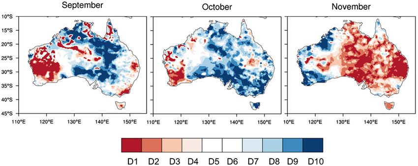
www.nature.com/scientificreports/
Figure 1. Large-scale conditions of the sea surface and the atmosphere in austral spring 2020. (a) September–
November mean (SON; i.e., spring) SST anomalies of 2020 relative to 1990–2012 climatology. The red and blue
boxed areas are the western pole and the eastern pole of the IOD, respectively; the long-dashed black boxed
area is the domain for the SSTs north of Australia considered in this study; and the blue boxed area over the
tropical Pacific shows the Niño3.4 region. (b) 700-hPa geopotential height anomalies of SON 2020. The short
dashed horizontal lines show 40°S and 65°S where nearly zonally symmetric meridional dipole of the SAM
is usually found. (c) Oceanic and atmospheric climate indices during the second half of 2020. The dark blue,
light blue, aqua blue, orange and purple bars indicate the monthly mean values of the Niño3.4 SST, the El Niño
Modoki index33, the Indian Ocean Dipole mode (IOD) index3, the SSTs north of Australia, and the SAM i ndex9,
respectively. Details of the climate indices shown in (c) are described in “Methods”. Maps were generated using
the NCAR Command Language version 6.6.2 (www.ncl.ucar.edu).
Scientific Reports | (2021) 11:18423 | https://doi.org/10.1038/s41598-021-97690-w 3
Vol.:(0123456789)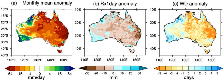
www.nature.com/scientificreports/
Figure 2. Rainfall decile map of spring 2020. The decile thresholds were obtained from the rainfall data over
1990–2012. A similar decile map but with the thresholds obtained from the full AWAP rainfall record since 1900
is available at http://www.bom.gov.au/climate/maps/rainfall/?variable=rainfall&map=decile&period=3month&
region=nat&year=2020&month=11&day=30. The map was generated using the NCAR Command Language
version 6.6.2 (www.ncl.ucar.edu).
Figure 3. Synthesis of 2020 spring rainfall anomalies using multiple linear regression onto key climate indices.
The contributions from the individual predictors are (a) de-trended Niño3.4 SST index, (b) de-trended DMI,
(c) de-trended SSTs north of Australia (eq-10°S,110–160°E), (d) de-trended SAM, and (e) time (i.e., trend). The
full synthesis using all five predictors is shown in (f). (g) Observed 2020 spring rainfall anomaly relative to the
climatology of 1990–2012. (h) Difference between the observed and the synthesized rainfall. The BoM official
base period is 1961–1990, and the anomaly pattern relative to this earlier base period is similar to (g) (http://
www.bom.gov.au/climate/maps/rainfall/?variable=rainfall&map=anomaly&period=3month®ion=nat&
year=2020&month=11&day=30). In (a)–(e) synthesis anomalies were computed by the regression coefficients
obtained over 1979–2019 and then scaled by the predictor values of 2020 (see “Methods”). Stippling in (a)–(e)
indicates where correlation between the rainfall and each predictor is statistically significant over 1979–2019 at
the 5% level. Maps were generated using the NCAR Command Language version 6.6.2 (www.ncl.ucar.edu).
Scientific Reports | (2021) 11:18423 | https://doi.org/10.1038/s41598-021-97690-w 4
Vol:.(1234567890)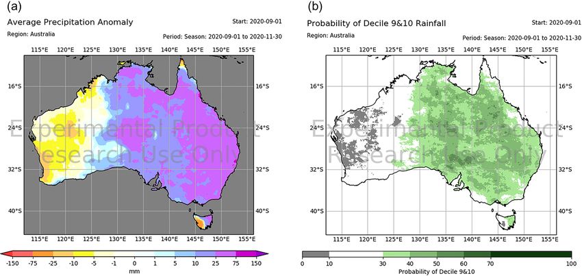
www.nature.com/scientificreports/
Figure 4. Observed and forecast climate indices and eastern Australian rainfall for spring 2020 (September–
November mean). The ACCESS-S1 99-member forecasts were initialised on 1 July, 1 August, and 1 September
(light blue bars) (see “Methods”for the details of the formation of the ensemble). The dark blue bars display
observed values. In (f) observed and forecast rainfall was averaged over eastern Australia (east of 140°E; EAU
rain).
The Bureau of Meteorology’s dynamical forecast system ACCESS-S118 skilfully predicted the occurrence of La
Niña in austral spring as judged by the forecast Niño3.4 SST and the associated spatial details of the tropical SST
anomalies as depicted by the negative EMI and positive SSTnAU with up to two months lead time (Fig. 4a, b, d).
However, the local SSTs north of Australia were predicted to be too warm, with the predicted positive anomaly
being almost two times greater than observed, when the forecasts were initialised on 1 July, 1 August, and 1
September (Fig. 4d). On the other hand, ACCESS-S1 predicted the weak negative IOD of spring only at zero
lead time (i.e., initialised on 1 September), having predicted neutral IOD conditions in earlier forecasts (Fig. 4c).
Positive SAM was correctly predicted from the beginning of July (Fig. 4e) likely due to its connection with La
Niña in the forecast because the anomalous strengthening of the stratospheric polar vortex in October–November
2020 was not predictable until late September (Supplementary Figs. S1b and S6).
Together with the forecasts of tropical Indo-Pacific SST conditions and positive SAM, spring rainfall over
central and eastern Australia was predicted to be significantly higher than normal from the initial conditions
of July onwards (Fig. 4f). These dynamical forecasts are broadly consistent with the statistical forecast based on
the historical relationships presented in Fig. 3. Even at zero lead time, ACCESS-S1 predicted eastern Australia
to be significantly wetter than average, and the forecast probability for spring rainfall in the top 20% category
(based on the hindcast period 1990–2012) was significantly higher than the climatological probability (i.e., > 20%)
(Fig. 5). Further analysis using 99-member ensemble forecasts indicates that the rainfall amount of individual
forecast members over eastern Australia was strongly determined by their SSTnAU forecasts (correlation (r) > 0.4
at lead times 0 and 1 month) and, to a lesser degree, by the EMI and SAM forecasts (r > 0.2 at lead times 0 and
1 month) (Supplementary Fig. S7).
Despite all these strong reasons to anticipate a wet spring, much less rain fell than was expected—more than
half of the country turned out to be drier than average (Fig. 3g) (relative to the mean climate of 1990–2012 in
this study, but this is also the case relative to the earlier period mean climate of 1961–1990; http://www.bom.gov.
au/c limat e/m
aps/r ainfa ll/?v ariab
le=r ainfa ll&m
ap=a nomal y&p
eriod=3 month
&r egion=n
at&y ear=2 020&m
onth=
11&day=30). Figure 2 shows that the spring rainfall deficit was particularly severe, being in the bottom 10–20%
of the climatological period of 1990–2012 in some locations of far eastern and south-eastern Queensland where
Scientific Reports | (2021) 11:18423 | https://doi.org/10.1038/s41598-021-97690-w 5
Vol.:(0123456789)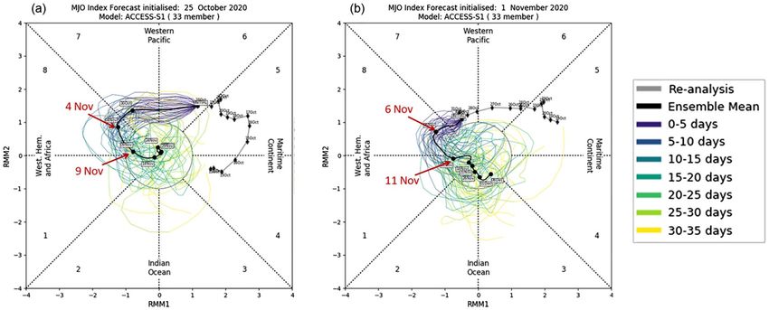
www.nature.com/scientificreports/
Figure 5. ACCESS-S1 99-member forecasts for spring rainfall, initialised on 1 September 2020. (a) Rainfall
anomaly and (b) probability of Decile 9 and 10 (i.e., top 20% category). Maps were generated with Python
version 3.6.1 (https://www.python.org/).
Figure 6. Rainfall decile maps of austral spring months. The decile thresholds were obtained from the period
1990–2012. Similar decile maps but based on the thresholds obtained from the full AWAP rainfall record since
1900 are available at http://www.bom.gov.au/climate/maps/rainfall/?variable=rainfall&map=decile&period=
month®ion=nat&year=2020&month=11&day=30. Maps were generated using the NCAR Command
Language version 6.6.2 (www.ncl.ucar.edu).
excessive rainfall was confidently predicted. Such a dry season was predominantly contributed to by significantly
below-normal rainfall in November 2020 (Figs. 6, 7a) when extreme dry conditions (i.e., bottom 10%) occurred
in all states and territories of Australia (Fig. 6), although the rainfall in September and October was also less
than expected (Fig. S8). In particular, there was a significant reduction in the number of rainy days (i.e., rain-
fall > 1 mm), which explains the extreme dry conditions in the Northern Territory and southern Queensland
with the latter location also being impacted by below-average maximum daily rainfall for the month (Fig. 7b, c).
So, why was November so dry in the midst of strong La Niña and associated SST conditions that were favourable
for a wet spring over eastern Australia?
Scientific Reports | (2021) 11:18423 | https://doi.org/10.1038/s41598-021-97690-w 6
Vol:.(1234567890)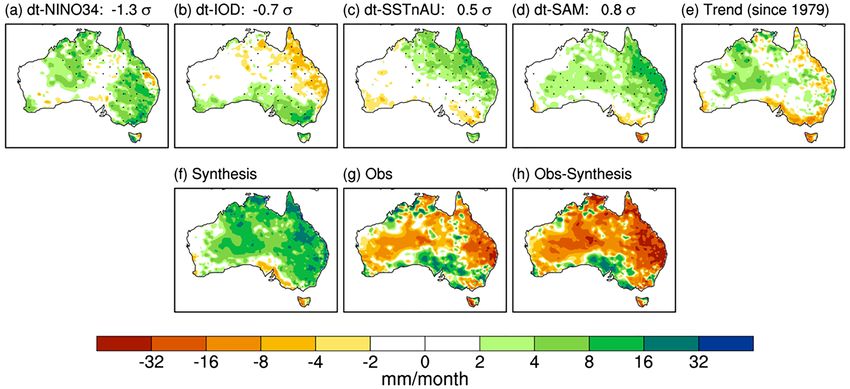
www.nature.com/scientificreports/
Figure 7. November 2020 rainfall anomalies. (a) Monthly mean, (b) 1-day maximum rainfall amount of the
month (Rx1day; i.e., the intensity of the wettest day in the month), and (c) number of wet days (> 1 mm; WD).
Maps were generated using the NCAR Command Language version 6.6.2 (www.ncl.ucar.edu) (a) and the IDL
version 8.6 (https://idlsgroup.com/) (b,c).
Figure 8. Madden–Julian Oscillation (MJO) in October-December 2020. Phase space of the Real-time
Multivariate MJO (RMM) index of Wheeler and Hendon (2004)40 for the period 1 October to 31 December
2020. Each dot represents a day and the sequence of days is joined by coloured lines. In October (red) the MJO
was primarily in Phases 5 and 6, in November (green) it was primarily in Phases 8, 1, 2, and 3, and in December
(blue) in Phase 5 and the Weak MJO circle.
November dryness over Australia
In addition to the dominant seasonal modes of variability described above, another key driver of Australian
weather and climate variability, the Madden–Julian Oscillation (MJO)38, was active on the sub-seasonal time
scale through spring 2020. The convective phase of the MJO passed over the Maritime Continent and the equa-
torial western Pacific in October and over the western hemisphere, Africa, and western-central Indian Ocean in
November 2020 (Fig. 8). Previous work exploring MJO teleconnections to Australian weekly climate anomalies
in each season has shown that during September–November, drier-than-normal conditions occur over eastern
and south-eastern Australia when the MJO convective activity is enhanced over the central Indian Ocean and
Scientific Reports | (2021) 11:18423 | https://doi.org/10.1038/s41598-021-97690-w 7
Vol.:(0123456789)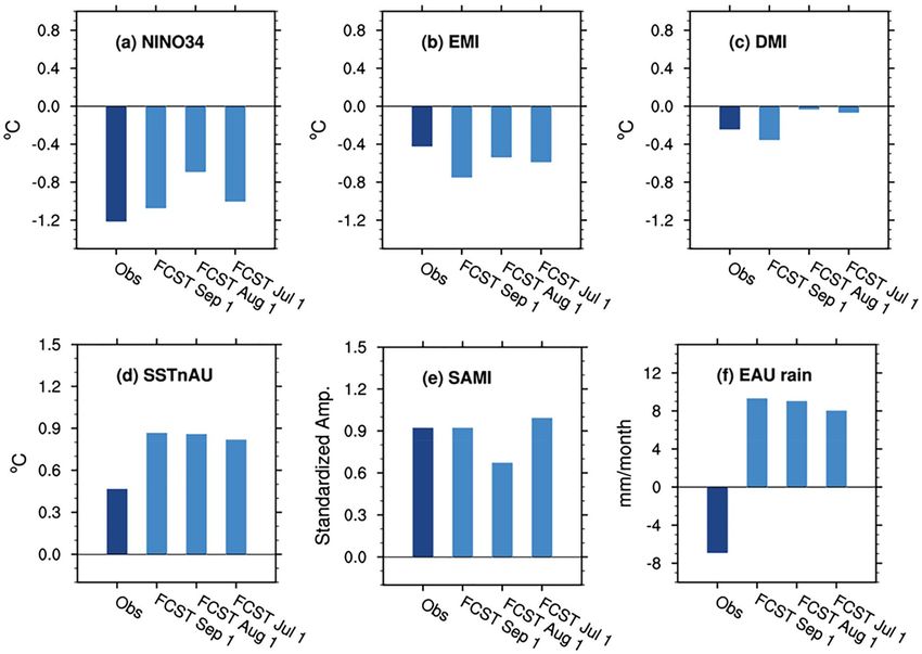
www.nature.com/scientificreports/
Figure 9. Time series of the sum of the daily MJO amplitudes for Phases 8, 1 and 2 during November (referred
to as MJO812). MJO amplitudes in Phases 8, 1, and 2 were summed only if they were equal to or greater
than 1 over more than one day in the month. The blue bars show the sum of the daily raw amplitudes for the
occurrence of Phases 8, 1, and 2, and the orange bars show the same but with the linear dependence on the
Niño 3.4 SST index removed. The black and orange coloured horizontal dashed lines indicate the mean and the
positive 1 standard deviation of the ENSO-free MJO812 time series from its mean, respectively.
suppressed over the far western Pacific. This is depicted as the MJO being in Phases 2 and 3 as displayed at http://
www.bom.gov.au/climate/mjo/#tabs=Average-conditions39.
In November 2020, the MJO propagated through Phases 7, 8, 1, 2, 3, and 4, with the most time and strong-
est amplitudes in Phases 8, 1, and 2. As a novel attempt to capture the impact of the MJO on the monthly total
rainfall in November 2020, we formed an index for November by summing the daily amplitudes of the MJO
in Phases 8, 1 and 2 (MJO812) whenever they were equal to or greater than one for more than one day in each
phase. We used the amplitude of the MJO based on the Real-Time Multivariate MJO (RMM) Index available at
the BoM40 (see “Methods”). In forming the MJO812 index, we removed the ENSO signal by linearly regressing
it out from the raw MJO812 index. Because the interannual variability was already removed from the RMM
indices40, the raw November MJO812 index is not statistically significantly correlated with the Niño3.4 SST index
at the 10% level, assessed by a two-tailed Student41 t-test with the 41 samples of 1979–2019. Nevertheless, some
of the high MJO812 activities occurred during strong El Niño years such as 1982 and 1997. Therefore, removing
the ENSO signal from the MJO812 index was appropriate to select the ENSO-free high MJO events. The raw
and the ENSO-removed MJO812 time series for November are shown in Fig. 9. The amplitude of the MJO812
anomaly during 2020 was about 1σ. Without the ENSO-related component, the November 2020 value was the
6th strongest in the recent 42-year record.
To understand the impact of high MJO812, we have made the composite differences of November-mean
outgoing long wave radiation (OLR) and Australian rainfall between the 6 highest amplitude MJO812 years
(1984, 1992, 1993, 1994, 1996, 2006) and the 8 lowest amplitude MJO812 years (1987, 1995, 1998, 2001, 2004,
2007, 2008, 2015). The years were selected based on the ENSO-free MJO812 index in Fig. 9 being greater than
|1σ|. The influence of ENSO on November-mean OLR flux and rainfall was also removed by regression before
making the composite differences.
High values of the MJO812 index are historically associated with November-mean enhancement of convec-
tion over the western to central equatorial Indian Ocean and suppression of convection over the eastern Indian
Ocean and the Maritime Continent (Fig. 10a). When MJO812 is high during November, the western half of
the Northern Territory/the eastern half of Western Australia and eastern Queensland, especially the southeast
corner of Queensland, experience extensive dryness compared to when MJO812 is anomalously low (Fig. 10b).
Strikingly, this rainfall pattern associated with high MJO activity in Phases 8, 1 and 2 matches well with the
extreme rainfall deficit during November 2020 (Figs. 6 and 7a), suggesting that the MJO activity over the Indian
Ocean and its teleconnection played a key role in acting to dry eastern Australia after the negative IOD decayed.
Composite differences of 1-day maximum rainfall amount and the number of wet days suggest that the number
of rainy days reduces over northern and north-eastern Australia when MJO812 is anomalously high, and both
number of rainy days and 1-day maximum rainfall amount significantly reduce over the southeast corner of
Queensland, where the dry response of the November mean rainfall to MJO812 is especially strong (Fig. 10c, d).
For the hindcast period of 1990–2012, ACCESS-S1 demonstrates skill in predicting the MJO, based on the
RMM indices, out to about four weeks lead time42. Seasonally, this skill extends to 30 days in austral winter and
spring and reduces slightly to 25 days in austral summer and autumn23. Together with this predictive skill of
the MJO, ACCESS-S1 also captures the observed modulation of extreme rainfall by the MJO in weeks two and
three of the f orecast23. This translates to enhanced skill for predicting MJO-related extreme rainfall across much
of Australia during spring and summer23. For instance, some of the largest forecast skill improvements in spring
are achieved for northern Australian rainfall during MJO Phase 8 and for central Australian rainfall during MJO
Phase 2 when the MJO is strong as compared to when it is weak. Moreover, in each of the MJO Phases 8, 1 and 2
the model shows useful skill (better than a random forecast) for predicting dry extremes over most of Australia
including the east (not shown). Thus, if ACCESS-S1 was to adequately predict the state of the MJO in November
Scientific Reports | (2021) 11:18423 | https://doi.org/10.1038/s41598-021-97690-w 8
Vol:.(1234567890)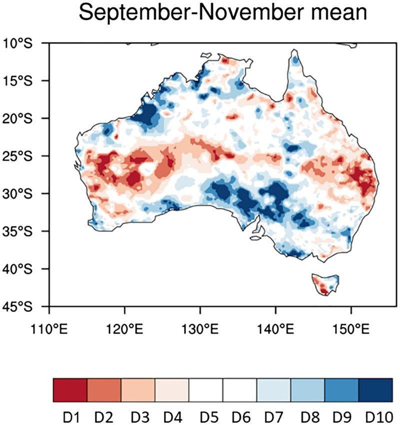
www.nature.com/scientificreports/
Figure 10. Composite difference between 6 highest and 8 lowest MJO812 indices during November. (a) Mean
outgoing long wave radiation (OLR), (b) monthly mean rainfall, (c) 1-day maximum rainfall amount, and (d)
number of wet days. Before forming the composites, the ENSO-related components were removed by regressing
out the linear dependence on the Niño3.4 SST index. The hatched areas in (a) and (b) and the black coloured
areas in (c) and (d) indicate statistically significant differences at the 5% level. In (c) and (d), the black shaded
differences in central Australia are unlikely to be a robust feature because it is a very dry area, and therefore,
differences could be dominated by one or two events, particularly given the small sample sizes in the two MJO
groups. Maps were generated using the NCAR Command Language version 6.6.2 (www.ncl.ucar.edu) (a,b) and
the IDL version 8.6 (https://idlsgroup.com/) (c,d).
2020 in its Phases 8, 1 and 2, it should have provided some indication of the dry conditions over Australia in the
forecasts made from the second half of October 2020.
The ACCESS-S1 ensemble mean forecasts for the MJO initialised in late October onwards were able to pre-
dict the amplification of the MJO in Phase 8 in the first 10 days of November (Fig. 11). However, as the spread
of the ensemble grew rapidly after that, the ensemble mean forecast MJO rapidly weakened and did not evolve
through Phases 1 and 2 during mid- to late November. This failure is likely to stem from the forecast MJO
being unable to maintain its suppressed convection over the Maritime Continent and the western Pacific where
anomalously enhanced convection was forced by the forecast La Niña. In reality, however, the MJO propagated
through that region (Supplementary Fig. S9). Consequently, the ensemble mean forecast for the MJO812 index
during November 2020 was only about half the strength of the observed (Fig. 12g). The 33-member ensemble
forecasts of northern and eastern Australian rainfall show some sensitivity to the forecast strength of MJO812
when they were initialised on 25 October, but it was much weaker than the observed (Supplementary Fig. S10).
While the MJO812 amplitude and its connection to Australian rainfall were significantly under-predicted,
La Niña and the associated westward shift of the maximum cold SST anomaly (as captured by EMI), the SST
anomalies to the north of Australia and the negative IOD were all over-predicted even at the shortest lead time
for the month of November (except for the IOD at 0 lead time) (Fig. 12b–e). Moreover, ACCESS-S1 significantly
over-predicted the positive SAM, with more than doubling of the observed strength that may result from too
strong downward coupling from the stronger-than-normal stratospheric polar vortex over Antarctica (Fig. 12f).
The forecast of overly strong positive SAM would have further raised the odds of increased rainfall over subtropi-
cal Australia and the odds of decreased rainfall over western Tasmania as ACCESS-S1 skilfully simulates the
SAM-Australian rainfall connection in late spring when the SAM forcing is s trong15. Therefore, it appears that
a combination of these different factors led to the over-prediction of wet conditions in subtropical Australia for
November 2020 (Fig. 12a).
Summary and concluding remarks
La Niña is well known to be associated with above normal rainfall over Australia and has often acted in the past
to terminate antecedent multi-year d roughts13,43–46. Furthermore, La Niña boasts long-lead predictability, even
beyond one year , that stems from the ocean wave dynamics known as the delayed oscillator48 or recharge-dis-
47
charge oscillator49, which is expressed at the sea surface as La Niña typically developing after strong El Niño. This
long-lead predictability of La Niña implies that the Australian rainfall component associated with La Niña should
Scientific Reports | (2021) 11:18423 | https://doi.org/10.1038/s41598-021-97690-w 9
Vol.:(0123456789)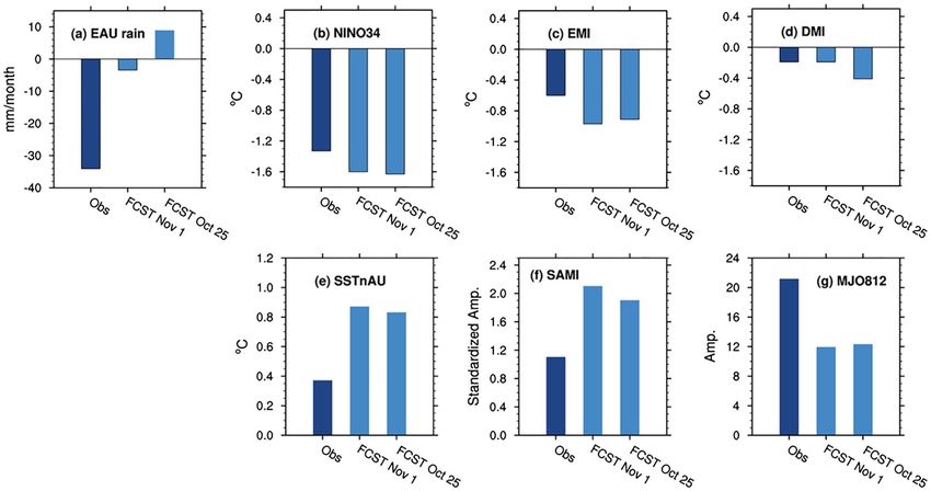
www.nature.com/scientificreports/
Figure 11. ACCESS-S1 forecasts for the MJO in November 2020. Forecasts were initialised on (a) 25 October
and (b) 1 November of 2020. A 33-member burst ensemble was used for these diagrams. The grey line indicates
the observed trajectory of MJO over the 15 days leading up to the forecast initialisation date, and the thick black
line indicates the ensemble mean forecast. The thin coloured lines indicate the ensemble member forecasts,
and the different colours denote the different verification windows as shown by the legend. The ensemble mean
forecasts shown in solid black lines are to be compared to the green line in Fig. 8.
Figure 12. ACCESS-S1 forecasts initialised on 25 October and 1 November 2020 for eastern Australian rainfall
and climate indices for November 2020. In (g) raw MJO812 (i.e., without removing its association with the
Niño3.4 SSTs) is displayed to simplify the comparison with the real-time forecasts.
be predictable at long-lead times. From mid-2020 international seasonal climate forecast models—both statisti-
cal and dynamical models alike—predicted the occurrence of La Niña with a moderate strength (0.5–1 °C at the
Niño 3.4 region) (https://i ri.c olumb
ia.e du/o
ur-e xpert ise/c limat e/e nso/) and a significant strength of the negative
IOD (http://www.bom.gov.au/climate/model-summar y/archive.shtml). Accordingly, Australia was predicted to
be wetter than normal for spring 2020 from the forecasts made from winter 2020 right up to the beginning of the
spring, and there was a strong consensus among international forecast models. However, this confident forecast
for excessive rainfall did not verify well with rainfall being near or below average in many locations, especially
over south-eastern Queensland. Incorrect forecasts, such as this for spring 2020, not only have a negative impact
Scientific Reports | (2021) 11:18423 | https://doi.org/10.1038/s41598-021-97690-w 10
Vol:.(1234567890)www.nature.com/scientificreports/
on user-confidence in seasonal forecasts but also have significant economic and social repercussions particularly
if they come at key decision times. For example, stakeholder feedback suggests that the wet outlook for November
2020 caused producers to rush grain harvests and work excessive hours, resulting in pressure on workers’ health
and safety to get the crops harvested before it rained (Adrian McCabe, Grain Producers South Australia, pers
comm). These types of situations can result in significant mental stress and considerable expense (e.g., having
to get in extra labour and equipment to harvest and transport grain). Therefore, in this study we have reviewed
the climate features of austral spring 2020 in detail, evaluated forecasts from the BoM’s ACCESS-S1 system, and
attempted to understand why Australia was not wet in its spring despite the occurrence of La Niña 2020 and why
the forecast system did not predict the abnormal dry response.
During spring 2020, the negative IOD did not strengthen through the season but started decaying from
August, which was substantially earlier than the typical life cycle of the IOD1. Furthermore, although the SSTs
north of Australia were warmer than normal, they were only a half the strength of the expected anomaly given
the magnitude of the Niño3.4 SST of spring 2020 and the local linear SST trend since 1979. Because La Niña
impacts Australian climate via (1) the strengthened Walker circulation, which is coupled to the warmer-than-
normal SSTs in the far western Pacific region, including the SSTs surrounding northern A ustralia50,51 and also
(2) via the concurrent negative IOD4,36,52, the moderate warming of the local SSTs north of Australia and the
early termination of the negative IOD are likely to have contributed to the drier-than-expected spring over many
areas of Australia in 2020 despite the presence of La Niña.
Moreover, the drying was pronounced in November, particularly over south-eastern Queensland and central
Australia as evidenced by rainfall totals falling in the bottom 20% of the historical record since 1900 in many
locations. We found that this dry anomaly was largely due to the strong MJO activity over the tropical Indian
Ocean, which was depicted as the 6 th strongest event in November by our novel MJO812 index that represents
the duration and strength of the MJO in Phases 8, 1 and 2 during the month. The composite differences of Aus-
tralian November-mean rainfall (as well as the 1-day maximum rainfall amount and the number of wet days)
between the high and low amplitude MJO812 years selected from the period 1979–2019 reveal that MJO812
is associated with strongly supressed monthly mean convection over the Maritime Continent and northern
and eastern Australia and so can significantly reduce rainfall there in November. This composite difference of
November rainfall for high and low MJO812 years matches the November rainfall anomaly of 2020 remarkably
well, confirming that the MJO was a key driver of the dry conditions that developed during November 2020.
According to the assessment of the ACCESS-S1 hindcasts42, skilful predictions of the MJO are possible out
to about four weeks, which means that the November MJO essentially represents unpredictable short time scale
"noise" for the seasonal climate forecasts issued at the start of September or earlier. This intrinsic limitation in
the predictability of the MJO probably explains why seasonal forecasts from all international models failed to
forecast drier-than-normal spring conditions of 2020. However, even when forecasts were initialised in early
November, ACCESS-S1 did not successfully predict the large MJO amplitudes in Phases 1 and 2 that were
observed in mid-late November 2020. Whether this forecast failure to sustain the eastward propagation of the
strong MJO in Phases 1 and 2 reflects a sensitivity to the other forecast atmospheric/sea surface conditions of
November 2020 as briefly discussed in the previous section or reflects a systematic bias of ACCESS-S153 needs
further investigation.
In contrast to the MJO prediction, ACCESS-S1 substantially over-predicted the positive SST anomalies to the
north of Australia for the spring months, which appears to have enhanced a forecast wet signal over northern
and eastern Australia. In addition, November SAM was predicted to be too strongly positive, which was likely
due to too-strong coupling with the Antarctic stratospheric polar vortex strengthening for forecasts initialised
in late October to early November. The under-prediction of the MJO and associated teleconnection might have
exacerbated the over-prediction of the positive SAM and SAM-driven rainfall over Australia for November.
In general, seasonal forecast systems have less skill in predicting SSTs outside of the tropical central to eastern
Pacific Ocean54. Although ACCESS-S1 performs significantly better than climatology or persistence with respect
to predicting monthly and seasonal climate variability, there is still much room for improvement. For instance,
to improve the forecast accuracy and reliability of rainfall over Australia, the forecast accuracy of the SSTs sur-
rounding Australia, the MJO and the SAM will have to be improved.
Although the impact of decadal variability on the climate of spring 2020 was not considered in this study, it is
worth mentioning that the earlier demise of the negative IOD despite the presence of La Niña during spring 2020
may have been influenced by the probable current cold phase of the Inter-decadal Pacific Oscillation (IPO)55,56
(Supplementary Fig. S11). In the most recent cold IPO mean state, the IOD and ENSO were found to be more
independent of each other in austral spring compared to the previous warm IPO mean s tate56. Carefully designed
forecast sensitivity experiments to the ocean initial conditions may shed some light on the impact of the ocean
mean state on this IOD event of 2020 and its predictability.
Finally, there is a hint of a long-term drying trend since 1979 over eastern Queensland, the south-eastern
Australian coast, western Tasmania, and southwest Western Australia according to Fig. 3e. This drying trend is
similar to that in winter, but it is not statistically significant at the 10% level in spring. In contrast, a long-term
wetting trend over north-eastern Western Australia in spring is statistically significant at the 5% level, which
resembles the summer rainfall trend. It is worth noting that the overall trend pattern bears some resemblance
to the projected rainfall change under increasing greenhouse gas emission scenarios using the models of the
Coupled Model Inter-comparison Project phase 6 (CMIP6)57. These weak to moderate linear trends of rainfall
in spring stem, in part, from the long-term trends in different seasonal climate drivers, some of which may
oppose each other to result in a smaller impact. For instance, there has been a weak positive trend in the IOD in
spring as mentioned earlier, which would act to reduce spring rainfall in the southern part of the country, while
there has been a strong positive trend in the SSTs north of Australia, which would act to increase spring rainfall
in the northern part of the country. As austral spring is the season when the large-scale climate drivers tend to
Scientific Reports | (2021) 11:18423 | https://doi.org/10.1038/s41598-021-97690-w 11
Vol.:(0123456789)www.nature.com/scientificreports/
have big swings in their positive and negative phases and significantly impact Australian seasonal climate, bet-
ter understanding the mechanisms of these large-scale modes of climate variability, their interactions with one
another, and their representation in climate prediction models will be key to understanding future changes in
Australian sub-seasonal to seasonal climate and its predictability.
Methods
Climate indices. In this study, ENSO is examined using the Niño 3.4 index and the El Niño Modoki Index
(EMI)33. The Niño 3.4 index is the area-averaged SST anomaly over the Niño 3.4 region (5°S-5°N, 190–240°E).
The EMI is used to detect the ENSO events that have the maximum SST anomaly near the dateline and is the
difference between the area-averaged central Pacific SSTs (10°S–10°N, 165–220°E) and the sum of the half of the
area-averaged eastern Pacific SSTs (15°S–5°N, 250–290°E) and western Pacific SSTs (10°S–20°N, 125–145°E).
The IOD is monitored by the Indian Ocean Dipole mode index (DMI)3, which is the difference of the area-
averaged SST anomalies in the western pole (10°S–10°N, 50–70°E) and the eastern pole (10°S-eq, 90–110°E).
The SSTs north of Australia (SSTnAU) was defined by the areal-mean SSTs over the domain of 10°S-equator
and 110–160°E, following the definition of Hendon et al.13.
The SAM index was obtained following Gong and Wang9’s definition, which is the difference of normalised
zonal-mean mean sea level pressure anomalies between 40°S and 65°S.
The Real-Time Multivariate MJO Index (RMM) consists of the expansion coefficients of the first two leading
modes of empirical orthogonal functions (EOFs) of the combined fields of daily 850 and 200 hPa zonal winds
and satellite-observed outgoing long wave radiation data over 15°S–15°N40 that capture the amplitude and the
eastward propagation of the MJO. The RMM data and comprehensive information about the MJO are available
at http://www.bom.gov.au/climate/mjo/.
Statistical synthesis using multiple linear regression. The synthesis (or reconstruction) of the Aus-
tralian rainfall anomalies of spring 2020, derived from multiple linear regression analysis (Fig. 3), are computed
as follows:
First, the multiple linear regression coefficients are obtained for the training period 1979–2019:
ŷt = bi xi,t
where t and i denote the training period and the number of predictors, respectively; ŷt is the synthesis of the
predictand y for the training period; bi is the regression coefficient of the i-th predictor, derived from least squares
fit regression; and xi,t is the time series of the i-th predictor in the training period.
Then, the synthesis for 2020 is obtained by plugging the predictor values of 2020 in the multiple linear regres-
sion model:
ŷ2020 = bi xi,2020
Statistical significance test. Statistical significance on correlation and regression was tested by a two-
tailed Student t-test with 41 samples of 1979–2019 data. Statistical significance on the difference of two means
of high vs low MJO812 cases was also tested by a two-tailed Student t-test but with six samples for high MJO812
and eight samples for low MJO812 events.
ACCESS‑S1 system. ACCESS-S1 is the Australian Bureau of Meteorology (BoM)’s dynamical sub-sea-
sonal to seasonal climate forecast system18, which is based on the UKMO GloSea5 system58. The atmosphere is
resolved on a ~ 60 km grid with 85 vertical levels, appropriately resolving the stratosphere. The ocean is resolved
at 25 km with 75 vertical levels. The atmosphere, land and ocean component models are coupled every three
hours.
The real-time forecasts using the operational system for September–November 2020 were initialised with the
atmospheric conditions from the BoM’s numerical weather prediction system and the ocean conditions provided
from the Met Office Forecast Ocean Assimilation Model (FOAM)59. The real-time system produces a 33-member
and a 11-member ensemble of multi-week and seasonal forecasts every day, respectively. Generation of forecast
products provided by the BoM Climate Service uses a lagged ensemble approach to form a 99-member ensemble
(9 consecutive days for the seasonal forecast products). For example, forecasts initialised on 1 September 2020
displayed in Figs. 4 and 5 use a 99-member ensemble, consisting of the 11-member forecasts from each day from
24 August to 1 September 2020.
Real-time forecast anomalies were computed against the hindcast climatology over 1990–2012. 11-member
hindcasts of ACCESS-S1 out to 6-month lead time are available at four different initialisation dates per month
(1st, 9th, 17th and 25th). The zonal and meridional winds, temperatures, humidity, surface pressure, and soil tem-
peratures were initialised using the European Centre for Medium-Range Forecasts Interim Reanalysis (ERA-
Interim) data60, while the model soil moisture was initialised with the climatology of ERA-Interim computed over
1990–201258. The ocean was initialised with the analysis from FOAM. The 11-member ensemble was produced
by perturbing the atmospheric initial c onditions18,61 and through the Stochastic Kinetic Energy Backscatter
scheme (SKEB2)62. To compute anomalies of real-time forecasts initialised over 9 consecutive days, we used the
climatology of the immediate prior hindcast date for each real-time forecast initialisation date. For example,
an anomaly of the real-time forecast initialised on 30 August 2020 was computed relative to the climatology of
hindcasts initialised on 25 August for 1990–2012.
Scientific Reports | (2021) 11:18423 | https://doi.org/10.1038/s41598-021-97690-w 12
Vol:.(1234567890)www.nature.com/scientificreports/
For the analysis of the November forecasts, 33-member burst ensemble forecasts (i.e., all initialised on the
same date) were used. Further details of the ACCESS-S1 model configuration, initialisation, ensemble generation
and forecast performance can be found in Hudson et al. studies18,61.
Data availability
Reynolds OI SST analysis set is available at https://psl.noaa.gov/data/gridded/data.noaa.oisst.v2.html. Hurrell
et al. (2008) SST analysis set is available at https://c limat edata guide.u
car.e du/c limat e-d
ata/m
erged-h
adley-n
oaaoi-
sea-surface-temperature-sea-ice-concentration-hurrell-et-al-2008. NOAA interpolated OLR dataset is available
at https://psl.noaa.gov/data/gridded/data.interp_OLR.html. JRA-55 set is available at https://rda.ucar.edu/datas
ets/ds628. AWAP rainfall data set is available at http://www.bom.gov.au/climate/maps/rainfall/?variable=rainf
all&map=totals&period=week®ion=nat&year=2021&month=03&day=29.
Received: 10 June 2021; Accepted: 30 August 2021
References
1. Zhao, M. & Hendon, H. H. Representation and prediction of the Indian Ocean dipole in the POAMA seasonal forecast model. Q.
J. R. Meteorol. Soc. 135, 337–352 (2009).
2. Santoso, A., Mcphaden, M. J. & Cai, W. The defining characteristics of ENSO extremes and the strong 2015/2016 El Niño. Rev.
Geophys. 55, 1079–1129 (2017).
3. Saji, N. H., Goswami, B. N., Vinayachandran, P. N. & Yamagata, T. A dipole mode in the tropical Indian Ocean. Nature 401, 360–363
(1999).
4. Cai, W. et al. Teleconnection pathways of ENSO and the IOD and the mechanisms for impacts on Australian rainfall. J. Clim. 24,
3910–3923 (2011).
5. Lim, E.-P. & Hendon, H. H. Causes and predictability of the negative Indian Ocean dipole and its impact on La Niña during 2016.
Sci. Rep. 7, 12619 (2017).
6. Hio, Y. & Yoden, S. Interannual variations of the seasonal march in the Southern Hemisphere stratosphere for 1979–2002 and
characterization of the unprecedented Year 2002. J. Atmos. Sci. 62, 567–580 (2005).
7. Byrne, N. J. & Shepherd, T. G. Seasonal persistence of circulation anomalies in the Southern Hemisphere stratosphere and its
implications for the troposphere. J. Clim. 31, 3467–3483 (2018).
8. Lim, E.-P., Hendon, H. H. & Thompson, D. W. J. Seasonal evolution of stratosphere-troposphere coupling in the Southern Hemi-
sphere and implications for the predictability of surface climate. J. Geophys. Res. Atmos. 123, 12002–12016 (2018).
9. Gong, D. & Wang, S. Definition of Antarctic Oscillation index. Geophys. Res. Lett. 26, 459–462 (1999).
10. Thompson, D. W. J. & Wallace, J. M. Annular Mode in the extratropical circulation. Part I: Month-to-month variability. J. Clim.
13, 1000–1016 (2000).
11. Lim, E.-P., Hendon, H. H. & Rashid, H. Seasonal predictability of the Southern Annular Mode due to its association with ENSO.
J. Clim. 26, 8037–8054 (2013).
12. Seviour, W. J. M. et al. Skillful seasonal prediction of the Southern Annular Mode and Antarctic ozone. J. Clim. 27, 7462–7474
(2014).
13. Hendon, H. H., Lim, E.-P., Arblaster, J. M. & Anderson, D. L. T. Causes and predictability of the record wet east Australian spring
2010. Clim. Dyn. 42, 1155–1174 (2014).
14. Lim, E.-P. et al. Tropical forcing of Australian extreme low minimum temperatures in September 2019. Clim. Dyn. 56, 3625–3641
(2021).
15. Lim, E.-P. et al. The 2019 Southern Hemisphere stratospheric polar vortex weakening and its impacts. Bull. Am. Meteorol. Soc.
102, E1150-1171 (2021).
16. Nguyen, H., Wheeler, M. C., Hendon, H. H., Lim, E.-P. & Otkin, J. A. The 2019 flash droughts in subtropical eastern Australia and
their association with large-scale climate drivers. Weather Clim. Extrem. 32, 100321 (2021).
17. BoM. Annual climate statement 2019. Available at: http://www.bom.gov.au/climate/current/annual/aus/2019/#:~:text=2019 was
Australia’s warmest year,1.33 °C in 2013.&text=Warming associated with anthropogenic climate,over one degree since 1910, (2020).
18. Hudson, D. et al. ACCESS-S1: The new Bureau of Meteorology multi-week to seasonal prediction system. J. South. Hemisph. Earth
Syst. Sci. 673, 132–159 (2017).
19. Hendon, H. H. & Lim, E.-P. Long lead prediction of the 2019 climate extremes. in the Australian Meteorological and Oceanographic
Society Annual Conference Abstracts p 269, https://d rive.g oogle.c om/fi
le/d/1 3uu4X
tHKcW
KcSTZ
f2aKc i_g NA0Hj Tikd/v iew, (2021).
20. Hudson, D. A. et al. ACCESS-S1 The new Bureau of Meteorology multi-week to seasonal prediction system. J. South. Hemisph.
Earth Syst. Sci. 67, 132–159 (2017).
21. King, A. D. et al. Sub-seasonal to seasonal prediction of rainfall extremes in Australia. Q. J. R. Metrol. Soc. https://doi.org/10.1002/
qj.3789 (2020).
22. Hendon, H. H., Lim, E.-P. & Abhik, S. Impact of interannual ozone variations on the downward coupling of the 2002 Southern
Hemisphere stratospheric warming. J. Geophys. Res. Atmos. https://doi.org/10.1029/2020JD032952 (2020).
23. Marshall, A. G., Hendon, H. H. & Hudson, D. Influence of the Madden-Julian Oscillation on multiweek prediction of Australian
rainfall extremes using the ACCESS-S1 prediction system. J. South. Hemisph. Earth Syst. Sci. https://doi.org/10.1071/ES21001
(2021).
24. Marshall, A. G., Gregory, P. A., de Burgh-Day, C. O. & Griffiths, M. Subseasonal drivers of extreme fire weather in Australia and
its prediction in ACCESS-S1 during spring and summer. Clim. Dyn. https://doi.org/10.1007/s00382-021-05920-8 (2021).
25. L’Heureux, M. L. & Thompson, D. W. J. Observed relationships between the El Niño-Southern Oscillation and the extratropical
zonal-mean circulation. J. Clim. 19, 276–287 (2006).
26. Lim, E.-P. & Hendon, H. H. Understanding and predicting the strong Southern Annular Mode and its impact on the record wet
east Australian spring 2010. Clim. Dyn. 44, 2807–2824 (2015).
27. Risbey, J. S., Pook, M. J., Wheeler, M. C. & Hendon, H. H. On the remote drivers of rainfall variability in Australia. Mon. Weather
Rev. 137, 3233–3253 (2009).
28. Reynolds, R. W., Rayner, N. A., Smith, T. M., Stokes, D. C. & Wang, W. An improved in situ and satellite SST analysis for climate.
J. Clim. 15, 1609–1625 (2002).
29. Hurrell, J. W., Hack, J. J., Shea, D., Caron, J. M. & Rosinski, J. A new sea surface temperature and sea ice boundary dataset for the
community atmosphere model. J. Clim. 21, 5145–5153 (2008).
30. Liebmann, B. & Smith, C. A. Description of a complete (interpolated) outgoing longwave radiation dataset. Bull. Am. Meteorol.
Soc. 77, 1275–1277 (1996).
31. Kobayashi, S. et al. The JRA-55 reanalysis: General specifications and basic characteristics. J. Meteorol. Soc. Japan. Ser. II(93), 5–48
(2015).
Scientific Reports | (2021) 11:18423 | https://doi.org/10.1038/s41598-021-97690-w 13
Vol.:(0123456789)www.nature.com/scientificreports/
32. Jones, D., Wang, W. & Fawcett, R. High-quality spatial climate data-sets for Australia. Aust. Meteorol. Oceanogr. J. 58, 233–248
(2009).
33. Ashok, K., Behera, S. K., Rao, S. A., Weng, H. & Yamagata, T. E. Niño Modoki and its possible teleconnection. J. Geophys. Res. 112,
C11007 (2007).
34. Deser, C., Phillips, A. S. & Alexander, M. A. Twentieth century tropical sea surface temperature trends revisited. Geophys. Res.
Lett. 37, 1–6 (2010).
35. Lim, E. P. et al. Interaction of the recent 50 year SST trend and La Niña 2010: Amplification of the Southern Annular Mode and
Australian springtime rainfall. Clim. Dyn. 47, 2273–2291 (2016).
36. Ummenhofer, C. C. et al. What causes southeast Australia’s worst droughts?. Geophys. Res. Lett. 36, L04706 (2009).
37. Abram, N. J. et al. Coupling of Indo-Pacific climate variability over the last millennium. Nature 579, 385–392 (2020).
38. Madden, R. A. & Julian, P. R. Detection of a 40–50 day oscillation in the zonal wind in the tropical pacific. J. Atmos. Sci. 28, 702–708
(1971).
39. Wheeler, M. C., Hendon, H. H., Cleland, S., Meinke, H. & Donald, A. Impacts of the Madden–Julian oscillation on Australian
rainfall and circulation. J. Clim. 22, 1482–1498 (2009).
40. Wheeler, M. C. & Hendon, H. H. An All-season real-time multivariate MJO index: Development of an index for monitoring and
prediction. Mon. Weather Rev. 132, 1917–1932 (2004).
41. Student. The probable error of a mean. Biometrika 6, 1 (1908).
42. Marshall, A. G. & Hendon, H. H. Multi-week prediction of the Madden–Julian oscillation with ACCESS-S1. Clim. Dyn. 52,
2513–2528 (2019).
43. McBride, J. L. & Nicholls, N. Seasonal relationships between Australian rainfall and the Southern oscillation. Mon. Weather Rev.
111, 1998–2004 (1983).
44. Power, S., Casey, T., Folland, C., Colman, A. & Mehta, V. Inter-decadal modulation of the impact of ENSO on Australia. Clim.
Dyn. 15, 319–324 (1999).
45. Holgate, C. M., Van Dijk, A. I. J. M., Evans, J. P. & Pitman, A. J. Local and remote drivers of Southeast Australian drought. Geophys.
Res. Lett. 47, (2020).
46. King, A. D., Pitman, A. J., Henley, B. J., Ukkola, A. M. & Brown, J. R. The role of climate variability in Australian drought. Nat.
Clim. Chang. 10, 177–179 (2020).
47. Luo, J.-J., Liu, G., Hendon, H., Alves, O. & Yamagata, T. Inter-basin sources for two-year predictability of the multi-year La Niña
event in 2010–2012. Sci. Rep. 7, 2276 (2017).
48. Battisti, D. S. & Hirst, A. C. Interannual variability in a tropical atmosphere-ocean model: Influence of the basic state, ocean
geometry and nonlinearity. J. Atmos. Sci. 46, 1687–1712 (1989).
49. Jin, F. & An, S. Within the equatorial ocean recharge oscillator model for ENSO. Geophys. Res. Lett. 26, 2989–2992 (1999).
50. Nicholls, N. The Southern Oscillation, sea-surface-temperature, and interannual fluctuations in Australian tropical cyclone activity.
J. Climatol. 4, 661–670 (1984).
51. van Rensch, P. et al. Mechanisms causing east Australian spring rainfall differences between three strong El Niño events. Clim.
Dyn. 53, 3641–3659 (2019).
52. Meyers, G., McIntosh, P., Pigot, L. & Pook, M. The years of El Niño, La Niña and interactions with the tropical Indian Ocean. J.
Clim. 20, 2872–2880 (2007).
53. Zhu, H., Maloney, E., Hendon, H. & Stratton, R. Effects of the changing heating profile associated with melting layers in a climate
model. Q. J. R. Meteorol. Soc. 143, 3110–3121 (2017).
54. Cottrill, A. et al. Seasonal forecasting in the pacific using the coupled model POAMA-2. Weather Forecast. 28, 668–680 (2013).
55. Zhao, M., Hendon, H., Oscar, A., Liu, G. & Guomin, W. Weakened Eastern Pacific El Niño predictability in the early twenty-first
century. J. Clim. 29, 6805–6822 (2016).
56. Lim, E.-P., Hendon, H. H., Zhao, M. & Yin, Y. Inter-decadal variations in the linkages between ENSO, the IOD and south-eastern
Australian springtime rainfall in the past 30 years. Clim. Dyn. 49, 97–112 (2017).
57. Grose, M. R. et al. Insights from CMIP6 for Australia’s future climate. Earth Futur. 8, e2019EF001469 (2020).
58. MacLachlan, C. et al. Global Seasonal forecast system version 5 (GloSea5): A high-resolution seasonal forecast system. Q. J. R.
Meteorol. Soc. 141, 1072–1084 (2015).
59. Waters, J. et al. Implementing a variational data assimila- tion system in an operational 1/4 degree global ocean model. Q. J. R.
Meteorol. Soc. 141, 333–349 (2015).
60. Dee, D. et al. The ERA-Interim reanalysis: Configuration and performance of the data assimilation system. Q. J. R. Meteorol. Soc.
137, 553–597 (2011).
61. Hudson, D. et al. Corrigendum to: ACCESS-S1: The new Bureau of Meteorology multi-week to seasonal prediction system. J.
South. Hemisph. Earth Syst. Sci. 70, 393 (2020).
62. Bowler, N. E., Arribas, A., Beare, S. E., Mylne, K. R. & Shutts, G. J. The local ETKF and SKEB: Upgrades to the MOGREPS short-
range ensemble prediction system. Q. J. R. Meteorol. Soc. 135, 767–776 (2009).
63. Henley, B. J. et al. A tripole index for the interdecadal Pacific Oscillation. Clim. Dyn. 45, 3077–3090 (2015).
Acknowledgements
This study is part of the Forewarned is Forearmed project, which is supported by funding from the Austral-
ian Government Department of Agriculture, Water and the Environment as part of its Rural R&D for Profit
programme. H. Zhu received funding from the Australian Government’s National Environmental Science Pro-
gramme (NESP), and A. King received funding from the Australian Research Council (DE180100638). C. de
Burgh-Day and M. Wheeler received support from the Northern Australian Climate Program (NACP) funded
by Meat and Livestock Australia, the Queensland Government, and University of Southern Queensland. We are
grateful to Dr Sugata Narsey at the BoM for his feedback on the initial version of the manuscript. We thank Dr
Oscar Alves and other members of the seasonal prediction teams at the BoM for their work in the generation
and curation of the ACCESS-S1 hindcast set. E. Lim thanks Ms Alison Griffiths for her input to the title of this
article. This research was undertaken on the NCI National Facility in Canberra, Australia, which is supported
by the Australian Commonwealth Government. The NCAR Command Language (NCL; http://www.ncl.ucar.
edu) version 6.4.0, IDL version 8.7.3, and Python version 3.6.1 were used for data analysis and visualization of
the results. We also acknowledge NCAR/UCAR, NOAA, the Japanese Meteorological Agency, and the BoM
for producing and providing the Hurrell et al. (2008) SST analysis, the OLR data, the JRA-55 reanalysis, and
the MJO RMM data, respectively, and Henley et al.63 and NOAA for the availability of the IPO Tripole Index.
Finally, we thank Dr Shuhei Masuda for convening the peer-review process and two anonymous reviewers for
their valuable feedback on the manuscript.
Scientific Reports | (2021) 11:18423 | https://doi.org/10.1038/s41598-021-97690-w 14
Vol:.(1234567890)You can also read