Tipping points induced by parameter drift in an excitable ocean model
←
→
Page content transcription
If your browser does not render page correctly, please read the page content below
www.nature.com/scientificreports
OPEN Tipping points induced
by parameter drift in an excitable
ocean model
Stefano Pierini1,2* & Michael Ghil3,4
Numerous systems in the climate sciences and elsewhere are excitable, exhibiting coexistence of
and transitions between a basic and an excited state. We examine the role of tipping between two
such states in an excitable low-order ocean model. Ensemble simulations are used to obtain the
model’s pullback attractor (PBA) and its properties, as a function of a forcing parameter γ and of the
steepness δ of a climatological drift in the forcing. The tipping time ttp is defined as the time at which
the transition to relaxation oscillations (ROs) arises: at constant forcing this occurs at γ = γc. As
the steepness δ decreases, ttp is delayed and the corresponding forcing amplitude decreases, while
remaining always above γc. With periodic perturbations, that amplitude depends solely on δ over
a significant range of parameters: this provides an example of rate-induced tipping in an excitable
system. Nonlinear resonance occurs for periods comparable to the RO time scale. Coexisting PBAs and
total independence from initial states are found for subsets of parameter space. In the broader context
of climate dynamics, the parameter drift herein stands for the role of anthropogenic forcing.
Sudden changes in behavior of a physical system have played an important role in the geosciences since the early
1950s1–4; see also Ghil et al.5. The study of such changes was systematically described, under the name of bifurca-
tions and associated regime c hanges6,7. More recently, the term “tipping points” has been introduced from the
social sciences8 into the climate sciences by Lenton et al.9 and has attracted considerable attention.
A useful distinction between bifurcations and tipping points (TPs), beyond the rhetorical effect of the latter,
does arise in the theory of dynamical systems with explicit time dependence in the forcing or coefficients. Such
systems are opposed to those without explicit time dependence, that can often be treated within the framework
of classical differentiable dynamical systems10,11. The latter are referred to as autonomous, the former in general
as nonautonomous. For nonautonomous systems one often makes also the distinction between random forc-
ing, which leads to random dynamical s ystems12,13, and purely deterministic forcing, which leads to dynamical
systems that are also termed simply as n onautonomous14. A more general theory that combines the deterministic
and random cases is also e merging15; Ghil & L ucarini16 provide a discussion of the latter in the climate context.
17
Kuehn , among others, has shown how TPs generalize bifurcations in the broader setting of nonautonomous
and random dynamical systems, by considering the detailed evolution of the system in the neighborhood of a
TP, while Ashwin et al.18 have classified this behavior into three broad classes:
(1) B-tipping or Bifurcation-due tipping—slow change in a parameter leads to the system’s passage through a
classical bifurcation;
(2) N-tipping or Noise-induced tipping—random fluctuations lead to the system’s crossing an attractor basin
boundary; and
(3) R-tipping or Rate-induced tipping—rapid changes lead to the system’s losing track of a slow change in its
attractors.
Further perspective is provided by Feudel et al.19 and Ghil20 on climate applications and by Ashwin, Feudel,
Wieczorek and c oauthors21–24.
The autonomous differentiable dynamical system’s framework has served the climate sciences well for sev-
eral decades1–4,6,25. It is mainly the recent interest in anthropogenic climate change and its interaction with the
1
Department of Science and Technology, Parthenope University of Naples, Centro Direzionale, Isola C4,
80143 Napoli, Italy. 2CoNISMa, Rome, Italy. 3Geosciences Department and Laboratoire de Météorologie
Dynamique (CNRS and IPSL), École Normale Supérieure and PSL University, Paris, France. 4Atmospheric
and Oceanic Sciences Department, University of California at Los Angeles, Los Angeles, CA, USA. *email:
stefano.pierini@uniparthenope.it
Scientific Reports | (2021) 11:11126 | https://doi.org/10.1038/s41598-021-90138-1 1
Vol.:(0123456789)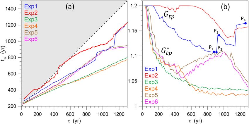
www.nature.com/scientificreports/
climate system’s natural variability that have led the research groups of Ghil and of Tél26–30, followed rapidly by
others, to introduce the framework of nonautonomous and random dynamical systems into the climate sciences.
In the context of nonautonomous dynamical systems, we analyze in the present study a problem that has
received relatively little attention to date: the tipping induced by a parameter drift in an excitable system, mark-
ing the transition from a stable basic state to self-sustained relaxation oscillations (ROs). Wieczorek et al.31
investigated such an effect in connection with the so-called compost-bomb instability, i.e., an explosive release
of soil carbon from peatlands into the atmosphere. Kiers and Jones32 and Wieczorek et al.33 analyzed conditions
for the occurrence of such R-tipping in excitable systems; see also applications of R-tipping to e cosystems21,23,24.
Before introducing in more detail the subject of the investigation and the model used, we briefly summarize
the concepts of multistability and excitability in climate dynamics. Multistability is one of the main paradigms
of climate dynamics6,16,25, in which the system possesses multiple equilibria, typically arising via saddle-node or
pitchfork bifurcations. Transitions from one equlibrium state to another can occur spontaneously if a threshold
is crossed, and subsequent bifurcations can lead to limit cycles, tori and strange attractors. Slow, quasi-adiabatic
changes in a parameter often lead to hysteresis between two stable equilibria. The transition from a nearly ice-free
climate to a snowball Earth and b ack16,34–36 is just one striking example of such behavior. The tipping induced by
parameter drift in multistable climate systems was studied, for example, by Drótos et al.28 and by Kaszás et al.37.
Another key paradigm of climate dynamics is provided by ROs and their excitability7,38,39. ROs are self-
sustained if a given threshold is passed, otherwise the system is said to be excitable, in which case ROs can be
excited by a stochastic p rocess40 through the so-called coherence resonance mechanism41. An excitable system
need not have multiple equilibria but must have a basic state that can be an equilibrium point, a small-amplitude
limit cycle or even a strange attractor occupying a small fraction of the phase space volume visited ultimately by
the trajectories. Whatever this basic state, the RO is composed of a rapid, large-amplitude transition that leads
the system to an unstable excited state and is followed by a spontaneous, slow return to the original basic state.
Relevant examples of paleoclimate and current climate phenomena that have been interpreted in terms of ROs
in excitable systems are: the ice ages over the late Pleistocene42, the Dansgaard-Oeschger events43–47, the Heinrich
events34,48,49, the multidecadal variability of the Atlantic Meridional Overturning Circulation ( AMOC50–53), and
the interannual variability of the Gulf Stream and Kuroshio E xtension54–61.
None of the studies above examined the phenomena under consideration from the unifying viewpoint of TPs
being crossed due to the gradual change in a key control parameter. Given the previously mentioned pervasive
effects of global warming, it is important to shed further light on its potential impact upon the interannual and
interdecadal variability of the Kuroshio Extension and AMOC, among other relevant manifestations of intrinsic
climate variability.
In this spirit, we study herein the four-variable wind-driven ocean model of P ierini62 and systematically
investigate its TPs under the action of a smooth drift in the external forcing. This low-order, spectrally truncated
quasigeostrophic model is nonlinear and excitable and the TPs mark its transition from an excitable to a self-
sustained RO regime. In our analysis, ensemble simulations (ESs) will be carried out to estimate the system’s
pullback attractors (PBAs) and to capture therewith its internal variability.
The model was originally developed to study aspects of the Kuroshio Extension dynamics that could not be
investigated with the much more realistic models based on the partial differential equations of geophysical fluid
dynamics because of the prohibitive computational cost required to do so. In fact, the affordable computational
cost of this low-order model did allow stochastic TPs to be s tudied63 and the system’s PBAs to be obtained in
several interesting c ases64–67. Apart from its original oceanographic application, the model should be seen here
as a mathematical tool used to investigate basic aspects of excitable systems, and the results so obtained could
be helpful in the broader context of the climate sciences and elsewhere.
The main issues addressed in the present study are: (a) finding the forcing amplitude at the TP and its depar-
ture from the corresponding frozen-in bifurcation value; (b) the analysis of the dependence of the TP on the
forcing’s drift rate; and (c) the sensitivity of the TP to the period and amplitude of periodic perturbations in the
forcing.
The paper is organized as follows. In the next section the mathematical model is described, an operational
definition of TPs is introduced, and the ES approach is discussed. In the subsequent sections, a basic numerical
experiment is presented and analyzed, several sensitivity experiments are discussed and, finally, the results are
summarized and conclusions are drawn.
Model and methods
The model and the experimental setup. The model used herein describes the wind-driven ocean cir-
culation in midlatitude basins, such as the North Atlantic or North Pacific. In such a circulation, a western
boundary current jet, such as the Gulf Stream in the North Atlantic, forms the common boundary of an anti-
cyclonic (i.e., clockwise in the northern hemisphere) subtropical gyre and a cyclonic (i.e., anticlockwise in the
northern hemisphere) subpolar gyre7,26,68. The analysis here is based on the highly truncated spectral double-
gyre model of Pierini62. The flow is two-dimensional and it is confined to a rectangular domain; it is described
by the streamfunction ψ(x, t), with ψ and the cartesian coordinates x = (x, y) being dimensionless. The time t
in the equations below is also dimensionless but we shall use in the text dimensional time, still denoted by t, to
emphasize the typical time scales of the oceanic phenomena that have inspired the model, namely the bimodal
decadal variability of the Kuroshio Extension55,69.
Our quasigeostrophic model is governed by four coupled nonlinear ordinary differential equations, written
here in vector–matrix notation as:
Scientific Reports | (2021) 11:11126 | https://doi.org/10.1038/s41598-021-90138-1 2
Vol:.(1234567890)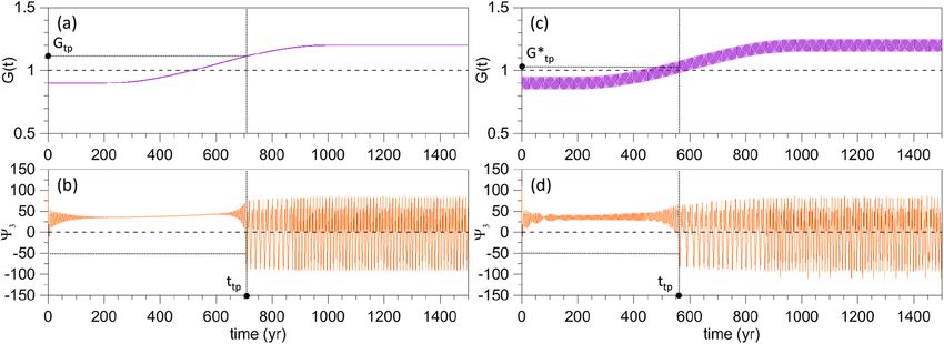
www.nature.com/scientificreports/
Figure 1. Definition of the ramp function Rτ (t); its duration is defined as τ = t2 − t1.
d�
+ �J� + L� = G(t)w; (1)
dt
here the vector �(t) = (�1 , �2 , �3 , �4 ) contains the coefficients in the truncated Galerkin expansion of the
streamfunction with respect to the orthonormal modes {Ei (x, y) : i = 1, . . . , 4}, with ψ(x, t) = 4i=1 �i (t)Ei (x, y).
ierini62 for the full evolution equation of ψ(x, t), the definition of the matrix operators J and L , the
Please see P
wind stress forcing vector w , the orthonormal basis {Ei (x, y)}, as well as for all the technical details and values
of the model parameters not mentioned here.
Moreover, Pierini62 noticed that 2 and 4 play a role similar to that of variables that are conjugate to 1 and
ierini62. Hence, the initial data in all the forward time integrations
3, respectively; see, for instance, Fig. 4 in P
are chosen to satisfy 1 = 2 and 3 = 464–66. Moreover, for the sake of convenience, the scaling 10−5 →
is adopted throughout.
The scalar factor G(t) in the external forcing of Eq. (1) is chosen as a linear combination of a normalized
climatological, time-independent component γ , a monotonic ramp, and a periodic perturbation:
G(t) = γ + αRτ (t) + β sin(ωt). (2)
Here γ , α and β are positive dimensionless constants, ω = 2π/T , while Rτ (t) is the ramp function shown
in Fig. 1, with τ = t2 − t1 and t1 = 200 year throughout the analysis; the explicit formula for Rτ (t) is given in
Supplementary Equation (S1).
This ramp is approximately linear near its midpoint and it varies smoothly towards the endpoints t1 and t2.
In our analysis, we will characterize the ramp by its steepness δ calculated at its midpoint:
δ = αRτ′ |t=(t1 +t2 )/2 . (3)
Keeping in mind the original application of model (1) to the Kuroshio Extension dynamics, the monotonically
increasing component in (2) stands for the effect of amplification in the midlatitude winds due to anthropogenic
warming, while the periodic perturbation can be thought of as the seasonal-to-interannual variability in the
westerly winds.
The behavior of the model’s autonomous version, in which α = β = 0, is discussed in the Supplementary
Information. The critical value γ = γc = 1 corresponds to a TP that marks the abrupt transition from small-
amplitude limit cycles to large-amplitude, nonlinear, self-sustained ROs; see Supplementary Figures S1, S2 and
discussion thereof. In particular, this sudden jump from a small- to a large-amplitude oscillation might be
associated with a canard-type transition70.
As an example of the two types of autonomous behavior, for γ < 1.0 and γ > 1.0, Fig. 2b, d illustrate the
evolution of �3 (t), initialized at the point marked by the red filled circle in Fig. 4 below. A very small-amplitude
periodic solution is plotted, for γ = 0.9, in panel (b) and a large-amplitude RO, for γ = 1.2, in panel (d) of
Fig. 2. In this autonomous case, the value γc = 1 that characterizes transition from small-amplitude oscillations
to large-amplitude ROs is identified by the light, black dashed line in panels (a, c).
It is worth stressing that ROs can emerge even for γ < γc: a suitable additive noise in G(t) can excite them and
thus activate coherence r esonance62; hence, γc = 1 identifies the upper bound of the so-called excitable regime.
Pierini63 introduced a stochastic TP γs to define the lower bound of this regime. A similar phenomenon was
described by S utera71 in the Lorenz convection m odel3, where it is associated with the existence of a subcritical
Hopf bifurcation; see Sec. 5.4 in ref.6 and Fig. 5.9 therein. In this earlier work, the role of the unstable RO here
is played by an unstable limit cycle.
In Supplementary Figure S3 and the related discussion, it is shown that our model possesses the fundamental
property of excitability when subjected to noisy forcing. This property is common to the excitable systems rele-
vant to the climate sciences mentioned in the introduction, ranging from p aleoclimatic34,42–49 to multidecadal50–53
54–61
and down to interannual time scales .
Tipping point definition for time‑dependent forcing. The question we want to answer in the pre-
sent study is: how does the transition from small-amplitude limit cycles to large-amplitude ROs occur if G(t) is
increased gradually from a subcritical value G < γc = 1 to a supercritical value G > 1? More specifically, at what
time and for what value of G does the abrupt transition occur? Figure 3 helps clarify this question.
Figure 3a shows the time dependence of G(t) for γ = 0.9. Thus, G passes gradually from its value in Fig. 2a to
that in Fig. 2c. The corresponding response is shown in Fig. 3b: the transition does not occur for G = 1, as one
might expect it; such a transition would require an infinitely slow increase of G(t), so as to take the system from
Scientific Reports | (2021) 11:11126 | https://doi.org/10.1038/s41598-021-90138-1 3
Vol.:(0123456789)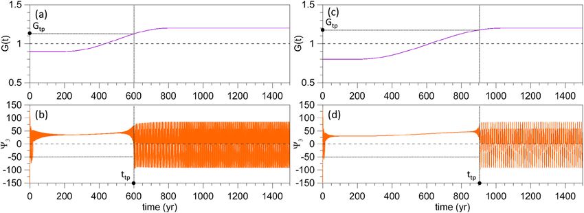
www.nature.com/scientificreports/

                                            Figure 2.  Typical solutions in the two regimes of the model’s autonomous version, cf. Eq. (1), with α = β = 0
                                            in the forcing given by Eq. (2). The constant values γ of the factor G(t) in the forcing are shown in the upper
                                            panels by a solid purple line, with (a) γ = 0.9 and (c) γ = 1.2. The corresponding model solutions are plotted
                                            for �3 (t) in the lower panels (b) and (d); see text and Fig. 4 for the initialization of the trajectories in the lower
                                            panels.

                                            Figure 3.  Transition from the excitable regime to the RO regime for a ramp forcing in Eq. (2). (a) Time
                                            dependence of the factor G(t) in the forcing for γ = 0.9 < γc = 1, α = 0.3, τ = 800 year, and β = 0; (b)
                                            corresponding response of �3 (t); see text for the choice of initial states. (c, d) Same as panels (a, b) but for
                                            β = 0.05 and perturbation period T = 5 year.

                                            the excitable regime to the RO regime adiabatically through a sequence of quasi-autonomous states. In fact, if
                                            we choose to identify the transition time—denoted here as the TP time ttp—as the one at which 3 is less than
                                            the threshold value 3,c = −50 for the first time, then the transition takes place at t = ttp = 707 year, which
                                            corresponds to G(ttp ) ≡ Gttp = 1.11 and is appreciably greater than γc = 1, cf. Fig. 3a, b.
                                               One might then wonder how robust this TP is. The simplest way to address this question is to add a sinusoidal
                                            perturbation to the ramp. In this case, i.e., if β = 0, we will use
                                                                                       G∗ (ttp ) ≡ Gtp
                                                                                                    ∗
                                                                                                       = γ + αRτ (ttp )                                          (4)
                                            to characterize the forcing amplitude at the TP. The example plotted in Fig. 3c, d differs from that of Fig. 3a, b
                                            only by the presence of such a perturbation in Eq. (2), with β = 0.05 and T = 5 year. As a result, ttp occurs earlier,
                                            at ttp = 563.5 < 707 year, whereas the amplitude is reduced to Gtp  ∗ = 1.029 < 1.11.
                                                 The methodology illustrated in Figs. 2 and 3 will be followed throughout our analysis, but the ESs mentioned
                                            in the introduction will be used to capture the system’s internal variability, as described in the next section.

                                            Ensemble simulations. For each time-dependent forcing G(t) used in this study, a 1500-year-long ES
                                            composed of N = 168 members will be carried out: this will provide an estimate of the system’s PBA. The initial
                                            points corresponding to the ensemble members will be regularly distributed at t = 0 in the four-dimensional
                                            hypercube  ≡ { −70 ≤ 1 , 2 ≤ 150; −150 ≤ 3 , 4 ≤ 120}. For the sake of graphical representation,we

          Scientific Reports |   (2021) 11:11126 |                https://doi.org/10.1038/s41598-021-90138-1                                                          4

Vol:.(1234567890)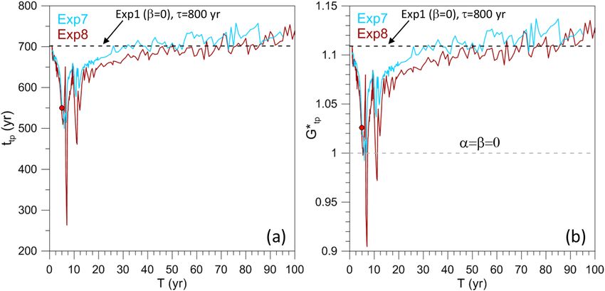
www.nature.com/scientificreports/
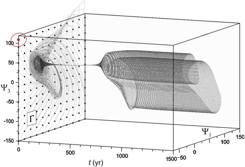
Figure 4. ES subject to the same forcing used in the single forward time integrations of Fig. 3a, b. The filled red
circle in the oval indicates the initial state used to initialize the four simulations of Figs. 2 and 3. After an initial
transient, it is visually obvious that the ES converges to a stable cylinder-shaped PBA, obtained by the translation
in time of an autonomous limit cycle.
Numerical experiment γ α τ (year) β T (year)
Exp1 0.9 0.3 32.5–1316.25 0 −
Exp2 0.8 0.4 ” ” −
Exp3 0.9 0.3 ” 0.025 5
Exp4 ” ” ” 0.050 ”
Exp5 0.8 0.4 ” 0.025 ”
Exp6 ” ” ” 0.050 ”
Exp7 0.9 0.3 800 0.050 1–100
Exp8 ” ” ” 0.100 ”
Table 1. List of the numerical experiments; see Eq. (2) for the definition of the parameters. In experiments
Exp1–Exp6, the duration τ = t2 − t1 of the ramp takes on 80 different values that range from 32.5 to
1316.25 year. In experiments Exp7 and Exp8, the period T ranges from 1 to 100 year. For each value of τ or T,
an ES with 168 initial states is carried out. Quotation marks in the table indicate identical entries.
will refer to the rectangle Ŵ ≡ { −70 ≤ �1 ≤ 150; −150 ≤ �3 ≤ 120} ⊂ � lying in the (�1 , �3 )-plane, as
done in P ierini64 and in subsequent analyses of model (1). Moreover, in the discussion of the results, we will refer
to the model’s trajectories as being defined in the (�1 , �3 )-plane but, naturally, the actual trajectories evolve in
the full four-dimensional phase space.
Figure 4 shows the ESs corresponding to the simulation of Fig. 3a, b, whose single integration is initialized
at the red point in the upper-left corner of Ŵ; the regular grid in Ŵ indicates the 168 initial points for the ES. The
definition of a TP for the time-dependent forcing introduced above is extended to an ES as follows: ttp is the time
at which, for the first time in any of the ES members, �3 < �3,c.
Results: the basic numerical experiment
In this section, a numerical experiment composed of 80 ESs is presented and discussed; it is denoted as Exp1
in Table 1 and it serves to study the TP’s dependence on the ramp steepness δ. For this study, we let τ take on
80 distinct values that range from very abrupt change in the forcing, with τ = 32.5 year, to very gradual, with
τ = 1316.25 year. Except for τ , all the other forcing parameter values in Eq. (2) here are the same as used for
the simulations in Figs. 3a, b and 4, namely γ = 0.9, α = 0.3 and β = 0. Moreover, for each τ -value, an ES with
168 initial data—such as that shown in Fig. 4—is carried out in order to simulate the irreducible uncertainty
associated with the system’s internal variability72–74. The ramps in G(t) for the two extreme values of τ are plotted
in Supplementary Figure S4.
Figure 5 summarizes the results of Exp1–Exp6, but we only discuss here those of Exp1; the results of
Exp2–Exp6 will be discussed in the following section. The blue line in Fig. 5a shows the dependence of ttp on τ
in Exp1: ttp increases monotonically and almost linearly with τ ; the anomalous jumps and fluctuations appearing
after t ≃ 1100 year will be explained below. The monotonically increasing trend is obviously due to the fact that
the greater τ the longer it takes to reach a given value of G.
The blue line in Fig. 5b shows that Gtp decreases almost linearly up to τ ∼ = 900 year as τ increases. Such a
negative trend is also expected because, as already observed, the slower the variation of the forcing strength the
closer the forcing at the TP will be to the autonomous critical value G = 1, i.e., we expect Gtp → 1 as τ → ∞.
Scientific Reports | (2021) 11:11126 | https://doi.org/10.1038/s41598-021-90138-1 5
Vol.:(0123456789)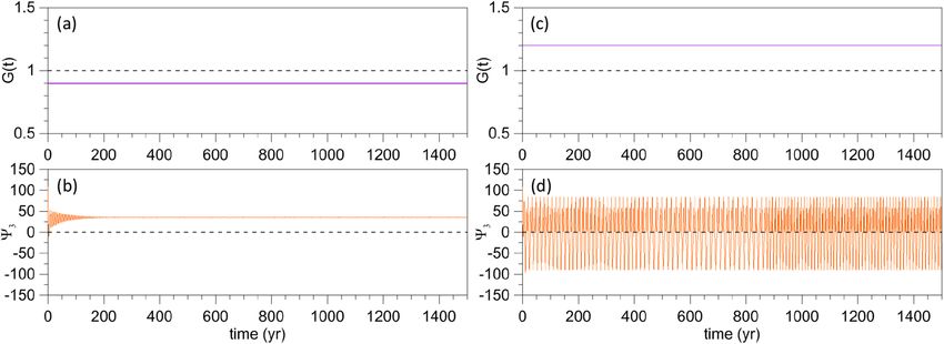
www.nature.com/scientificreports/

                                            Figure 5.  Dependence of key results on the ramp duration τ in experiments Exp1–Exp6. (a) TP timing ttp
                                            versus τ ; when a line portion lies in the grey area the tipping occurs after the end of the ramp. The filled circles
                                            on the red line indicate the presence of data; their absence indicates that no TP is reached. (b) Forcing values
                                            G(ttp ) at the TP (for Exp1 and Exp2) or Gtp ∗ (for Exp3–Exp6) versus τ ; the filled blue circles P −P correspond
                                                                                                                                               1  3
                                            to the ESs for Exp1 shown in Supplementary Figure S5, while the filled circle P4 corresponds to the orange ES of
                                            Supplementary Figure S6.

                                            Figure 6.  Same as Fig. 5b but shown as a function of the ramp steepness δ defined in Eq. (3). The solid black
                                            vertical line in the zoomed inset indicates the ramp steepness δ corresponding to the two ESs of Exp1 (blue line)
                                            and Exp2 (red line) shown in Fig. 8.

                                                It is important, though, to stress that the range of variability of the ramp’s duration τ considered herein spans
                                            time intervals that range from roughly 3 to roughly 130 times the typical time scale of the ROs; hence Gtp is
                                            always substantially greater than unity. Note that the initial plateau for τ ≤ 130 year in Fig. 5b is present because
                                            for those values the TP is reached at t > t2, i.e., when G = 1.2.
                                                Thus, in the range 130 year < τ < 900 year, as τ increases—and therefore the forcing’s drift rate δ decreases—
                                            the TP is delayed and the corresponding G-value decreases, but it remains well above the autonomous critical
                                            value G = 1. For τ > 900 year, a sudden increase of Gtp occurs in Fig. 5b, followed by a gradual decrease and
                                            another sharp increase. We investigate these anomalous behaviors in the Supplementary Information (see Sup-
                                            plementary Figures S5, S6 and S7).
                                                According to Fig. 5a, as τ increases, the TP is delayed and the corresponding value of Gtp in Fig. 5b decreases.
                                            It follows that, since increasing τ the ramp steepness δ decreases, Gtp must increase with δ. This increase is shown
                                            in Fig. 6 for Exp1 by the blue line: the forcing amplitude Gtp at the TP increases steeply and monotonically with

          Scientific Reports |   (2021) 11:11126 |               https://doi.org/10.1038/s41598-021-90138-1                                                     6

Vol:.(1234567890)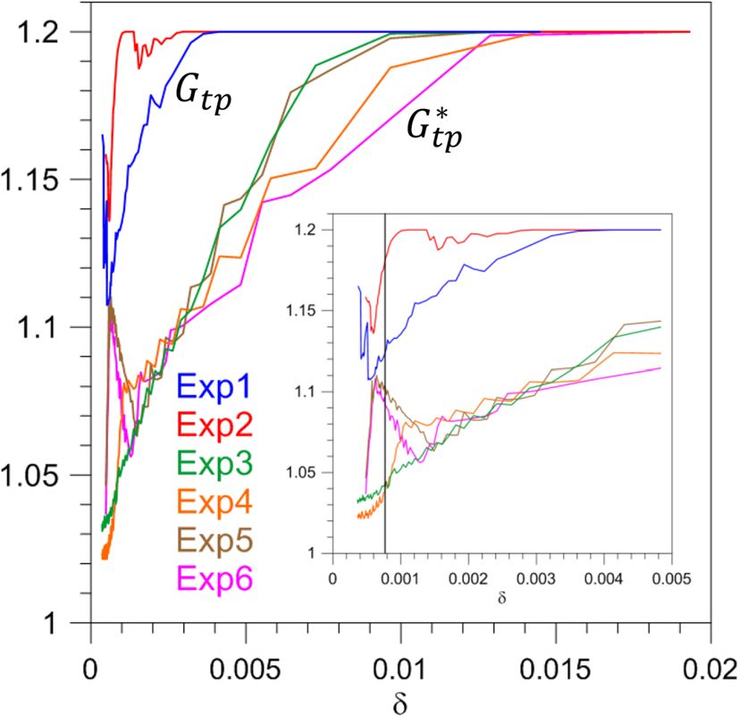
www.nature.com/scientificreports/
Figure 7. Dependence of the number C̄ of trajectory clusters on τ for Exp1, with T0 = 50 year and r = 0.5
in Eq. (6). The magenta, green and red bars refer to the ESs shown in Supplementary Figures S5, S6 and S8,
respectively.
the drift rate, except for the anomalous behavior found for δ < 0.0005 and δ > 0.004. The latter nonmonotonici-
ties are associated with the appearance and disappearance of local PBAs (see the Supplementary Information).
To complete the analysis of Exp1 we investigate the sensitivity to initial data of the ES members. Supple-
mentary Figures S5, S6 and S7 show that the RO phases tend to cluster in groups or may even exhibit total
independence from the initial data (TIID), as occurs in Supplementary Figure S5(b) for some of the N trajec-
tories. To obtain information about the phase dependence of the ensemble members, we rely on the parameter
C introduced by P ierini64:
N
1
(j)
C(r, t, τ ) = H r −
�τ(i) (t) − �τ (t)
; (5)
2
N i,j
here H is the Heaviside step function and r is a prescribed distance. This functional C gives the number of tra-
jectory pairs whose distance is less than r, normalized by N 2. In general, if the N available trajectories reduce to
n clusters, each one containing trajectories within the maximum distance r, then 1/n ≤ C ≤ 1. In the present
analysis each of these clusters will be denoted as “single trajectory” if r ≤ r0 = 0.5; r0 is in fact much smaller than
the projection of the PBA onto the Ŵ-plane. Note that the extreme case C = 1/n occurs if the N trajectories are
equally distributed among n single trajectories.
The particularly interesting case C = 1 (n = 1) implies TIID and is usually referred to as generalized synchro-
nization when the forcing is periodic, because then the unique single trajectory is necessarily synchronized with
the forcing (e.g.,64,75,76). More generally, the existence of a small number of single trajectories is clearly a case of
phase synchronization77–79.
A time-independent parameter can be obtained by averaging C over an interval T0 starting from the tipping
time ttp:
ttp (τ )+T0
1
C̄(r, τ ) = C(r, t, τ )dt. (6)
T0 ttp (τ )
Figure 7 shows C̄(r, τ ) with r = r0 = 0.5 and T0 = 50 year. See Supplementary Figure S8 for a discussion of
the four red bars. As τ is increased further in Fig. 7, the C̄-values for the ESs reported in Supplementary Fig-
ures S5 and S6 are plotted as the magenta and green bars, respectively. In particular, the unstable trajectories
corresponding to τ = 1300 year (cyan lines in Supplementary Figures S6 and S7(b)) yield a value of C̄ = 0.96
close to TIID, as expected.
Results: sensitivity experiments
In this section, we study the experiments Exp2–Exp8 summarized in Table 1, focusing on the changes in TPs
induced by the changes in the parameters γ , α, β and τ of the forcing in Eq. (2).
Sensitivity of tipping to the system’s past history (Exp2). In Exp1, we saw that the TP depends cru-
cially on the ramp steepness δ of the forcing G(t), which one can also think of as the drift rate; see again Figs. 5
and 6. Ashwin et al.18 defined rate-induced tipping for systems possessing multiple steady states16,80; the blue line
of Fig. 6 illustrates a similar phenomenon occurring in our excitable system for Exp1.
However, a natural question arises: does the TP depend solely on δ, as the R-tipping terminology suggests, or
does it dependent also—and perhaps crucially—on other parameters, too? To clarify this issue, we designed and
performed Exp2: it differs from Exp1 in that the climatological amplitude in Eq. (2) is reduced from γ = 0.9 to
γ = 0.8, while the ramp factor is increased from α = 0.3 to α = 0.4. As a consequence, Exp1 and Exp2 share the
same Gmax while, for a given τ , δ is larger in Exp2 then in Exp1. We will therefore be able to compare ESs with
the same δ but with a different past history.
Scientific Reports | (2021) 11:11126 | https://doi.org/10.1038/s41598-021-90138-1 7
Vol.:(0123456789)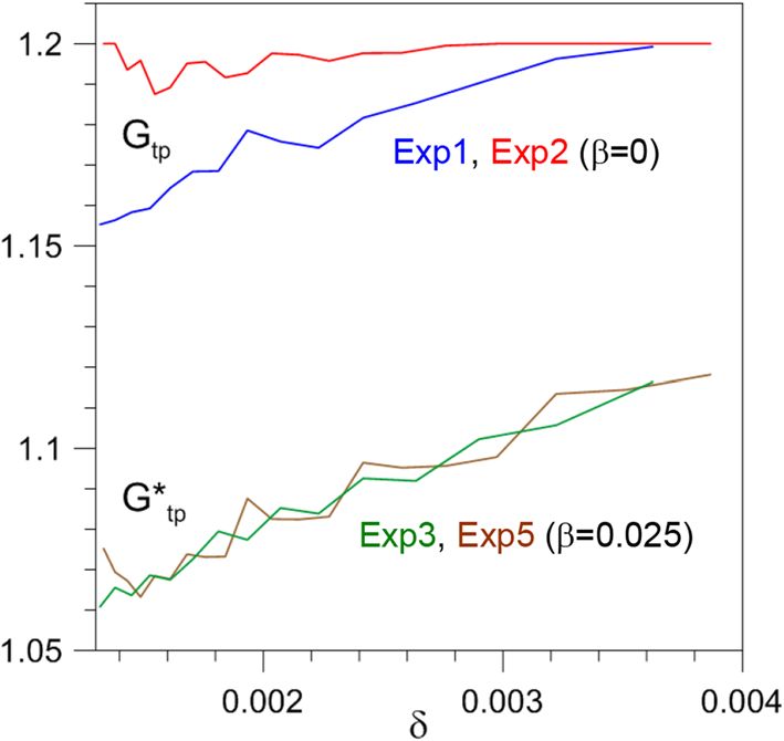
www.nature.com/scientificreports/

                                            Figure 8.  Dependence of the TP on ramp length for two ESs belonging to Exp1 and Exp2 and having the same
                                            drift rate δ. (a) Time dependence of the factor G(t) for Exp1 with τ = 600 year. (b) �3 (t) of the corresponding
                                            ES. (c) Time dependence of the factor G(t) for Exp2 with τ = 835 year. (d) �3 (t) of the corresponding ES.

                                                In Fig. 8, the details of an ES that is part of Exp1 are thus compared with those of an ES within Exp2. The
                                            two are chosen so that δ is the same in both, as shown by the vertical solid line in the zoomed inset of Fig. 6, but
                                            their past histories differ. In Exp2, both ttp and Gtp are found to be greater than in Exp1. More generally, the red
                                            solid lines of Exp2 are quite distinct from, and lie well above, the blue solid lines for Exp1 in both Figs. 5 and 6,
                                            where the dependence of ttp and Gtp on τ and δ, respectively, is plotted.
                                                Thus, in the case of forcing that increases monotonically, the transition is not determined by the drift rate
                                            δ alone but by both δ and the initial forcing amplitude. More precisely, based on the comparison between the
                                            dependence of Gtp on past history at given δ for Exp1 and Exp2, as shown in Fig. 6, we can conclude that the
                                            smaller the forcing amplitude γ < 1 at the beginning of the ramp, the greater the forcing amplitude at the TP
                                            has to be.
                                                This result clearly implies a long memory of the past. For example, let us consider the ESs of Exp1 and Exp2
                                            shown in Fig. 8. Suppose that, in Exp1, at t = ta the model has not yet reached the TP for G(ta ) = Ga ; then sup-
                                            pose that, in Exp2, at t = tb the model has not yet reached the TP either for the same G(tb ) = Gb = Ga . Still,
                                            Fig. 8b, d show that, shortly before the TP, the state of the system is virtually the same in both ESs.
                                                In summary, at t = ta in Exp1 and at t = tb in Exp2, the state of the system is virtually the same, δ is the same,
                                            while the value of the external forcing and its future evolution are the same as well. Yet the TP is reached at very
                                            different times with respect to the beginning t1 of the changes in the forcing. Since the only difference between
                                            Exp1 and Exp2 is the temporal evolution prior to ta and tb , respectively, this effect can only occur if the system
                                            keeps track of the previous evolution for sufficiently long times. One might expect that, if the system is perturbed,
                                            such an anomalous behavior would no longer occur.
                                                We will see in the next subsection that, in fact, if the forcing is perturbed by a periodic component, the sce-
                                            nario just discussed changes drastically. Namely, over a wide range of δ-values, the TP depends solely on δ. The
                                            latter behavior represents, therefore, a case of R-tipping in an excitable system.
                                                Finally, notice that, unlike in Exp1, C̄ ≃ 1 in Exp2, and thus the latter exhibits TIID for many more values
                                            of τ , as seen by comparing Supplementary Figure S9 with Fig. 7. An example is provided by the ES of Fig. 8d,
                                            in which the N ensemble members are well synchronized. The reason for such a difference in behavior deserves
                                            to be analyzed in detail in a future study. In the next subsection, we will at least investigate whether the TIID
                                            observed in Exp2 is stable or not.

                                            Sensitivity to periodic perturbations (Exp3–Exp6). It is important to assess the robustness of the
                                            results obtained in Exp1 and Exp2 with respect to perturbations of the forcing. We saw that a small-amplitude
                                            periodic perturbation added to the forcing can affect considerably ttp and Gtp  ∗ , cf. Figs. 3c, d, while Supplementary
                                            Figure S7 shows that even when such a periodic perturbation acts only over a short duration it may trigger an
                                            instability in the solution. Therefore, we now repeat Exp1 and Exp2 by adding periodic perturbations in G, with
                                            β = 0 in Eq. (2). The perturbation period is 5 year and we use two amplitudes, β = 0.025 and 0.05. Exp3 and
                                            Exp4 correspond to Exp1, while Exp5 and Exp6 correspond to Exp2; see Table 1.
                                                Compare now in Fig. 5 (1) the curve of Exp1 (blue) with those of Exp3 (green) and Exp4 (orange) and (2)
                                            that of Exp2 (red) with those of Exp5 (brown) and Exp6 (magenta). From panel (a) it is immediately clear that,
                                            as a result of the perturbation, ttp occurs notably earlier, while panel (b) clearly shows that the forcing amplitude
                                              ∗ is notably reduced. Note also that the difference (1) between Exp3 and Exp4 and (2) between Exp5 and Exp6
                                            Gtp
                                            is quite small, despite their perturbation amplitudes differing by a factor of 2.
                                                These two findings suggest that the TPs that are due to a drift in the forcing, as in Exp1 and Exp2, are unsta-
                                            ble: a small periodic perturbation shifts the TPs to values that are then robust with respect to changes in the
                                            perturbation’s amplitude. This result will be analyzed in greater depth in a future study and we strongly suspect
                                            that similar sensitivity to random, rather than periodic, perturbations will be also detected.

          Scientific Reports |   (2021) 11:11126 |                https://doi.org/10.1038/s41598-021-90138-1                                                      8

Vol:.(1234567890)
www.nature.com/scientificreports/
Figure 9. Rate-induced tipping in the presence of periodic perturbations. Same as Fig. 6 but for a limited range
of δ-values for the unperturbed (Exp1 and Exp2) and corresponding perturbed (Exp3 and Exp5) cases with
β = 0.025 and T = 5 year.
Another significant example of the instability of the unperturbed Exp1 and Exp2 concerns the dependence
of Gtp on δ. We saw big differences between Exp1 and Exp2 (blue and red lines in Fig. 6) in this dependence. On
the other hand, we argued there that, since such differences seem to be associated with the system’s full history,
the same value Gtp ∗ (δ) could result if the two histories of the forcing were subjected to a periodic perturbation.
This is in fact what occurs for a significant range of δ-values. Let us focus on δ ≥ 0.0013 in Fig. 6, which is
beyond the range of anomalous behaviors discussed in connection with the basic numerical experiment. The
lines showing Gtp (δ) for the unperturbed Exp1 and Exp2 and the lines showing Gtp ∗ (δ) for the corresponding
perturbed Exp3 and Exp5 with β = 0.025 are again reported, for 0.0013 ≤ δ ≤ 0.004, in Fig. 9. For the sake of
clarity, Exp4 and Exp6, with β = 0.05, are not plotted, since they yield basically the same behavior.
The first striking difference between the unperturbed and perturbed cases concerns the substantially smaller
values attained by the forcing amplitude at the TP for the perturbed cases, as just discussed. For values of the drift
rate approaching δ ≃ 0.004, the blue and red lines of Exp1 and Exp 2 both tend to the constant value Gtp = 1.2
because, as already noted, in this limit the TP is reached at t > t2 when G = 1.2. For decreasing δ the difference
between the two curves increases, as already discussed.
On the contrary, the lines (green and brown) showing Gtp ∗ (δ) for Exp3 and Exp5 essentially coincide in this
range. The memory of the remote past states of the perturbed system is lost, and the same forcing amplitude at
the TP is reached in Exp3 and Exp5—which, like Exp1 and Exp2, share the same mean drift rate. In conclusion,
the green and brown lines of Fig. 9 show a case of R-tipping in an excitable system.
In the Supplementary Information, interesting results are presented concerning the dependence of the phase
distribution of ROs on the presence and amplitude of periodic forcing (see Supplementary Figures S10 and S11).
Sensitivity to forcing period (Exp7 and Exp8). In the preceding subsection, we have studied the effect
of a periodic perturbation of fixed period T = 5 year on the TPs induced by a drift in the forcing for varying τ . In
order to analyze the sensitivity to forcing period, Exp1 is modified in Exp7 and Exp8 to include a periodic forc-
ing in which τ = 800 year is fixed, while the period T varies from 1 to 100 year; see again Table 1. The depend-
ence of the TP on T in these two numerical experiments is shown in Fig. 10. Like in the previous numerical
experiments we compute 80 ESs—in this case with T-values regularly distributed in the range 1–100 year—to
construct the graphs of Fig. 10. Many additional ESs are also computed for T = 1–25 year so as to capture the
strong variability of ttp and Gtp
∗ in this range.
Let us first focus on Exp7 (light blue lines), which shares the forcing amplitude β = 0.05 with Exp4. For high
values of T, ranging between 25 and 100 year, ttp and Gtp ∗ are close to the corresponding value of Exp1, with no
periodically perturbed forcing (black dashed line). For T ≃ 10–25 year the TP occurs somewhat earlier, while
for T < 10 year abrupt drops in ttp do occur. The biggest drop is at T ∼ = 6 year and it corresponds to an earlier
occurrence of the TP by about 200 year with respect to the periodically unperturbed case. For even smaller
T, ttp and Gtp
∗ return to their unperturbed values, while passing through the values that correspond to Exp4 at
T = 5 year; the latter values are indicated by a red filled circle.
A similarly anomalous behavior is found in Exp8 for the perturbation’s amplitude β being doubled (brown
lines in Fig. 10); in this case the sensitive dependence on the period T is even more striking. Chekroun et al.81
studied such a rough parameter dependence in a truncated version of a periodically driven, intermediate cou-
pled ENSO m odel82,83 by using the Ruelle–Pollicott resonances of the model’s associated Perron–Frobenius or
transfer operator84,85.
In the ENSO case of Chekroun et al.81, the period of the forcing was fixed and given by the seasonal cycle,
while the parameter δ of interest affected the travel time of the equatorially trapped waves and hence the intrin-
sic model periodicity. On the other hand, in the present case the intrinsic period of the ROs is determined
by the system’s dynamics, while the external-forcing period is being modified. But it is really the ratio of the
Scientific Reports | (2021) 11:11126 | https://doi.org/10.1038/s41598-021-90138-1 9
Vol.:(0123456789)www.nature.com/scientificreports/
Figure 10. Dependence of the TP on period T in Exp7 and Exp8. (a) TP timing ttp versus period T. The
horizontal dashed line indicates the value corresponding to Exp1 for τ = 800 year. (b) Gtp ∗ versus T. Black
dashed line as in panel (a), while the gray dashed line corresponds to the critical value of the autonomous
system. The red filled circles in both (a) and (b) indicate the value that is common to Exp7 and Exp4.
external-to-internal frequency that matters, as illustrated in the highly simplified case of Arnold tongues in the
standard circle map86,87.
Returning to Fig. 10 (brown line), two peaks at T ∼ = 7 year and T ∼= 11.2 year are found in Exp8 and, in both
cases, Gtp
∗ < 1: that is, the ROs arise for a time-averaged forcing amplitude that is appreciably smaller than the
value required for the autonomous system to transit from the excitable to the self-sustained RO regime.
The abrupt reduction of ttp and Gtp∗ occurs for periods T that are comparable to the RO’s typical time scale;
thus, we are in the presence of a nonlinear-resonance–like behavior. These results deserve further investigation
by relying on some of the tools discussed in connection with the ENSO case above.
Summary and conclusions
Excitable dynamical systems are characterized by large-amplitude relaxation oscillations (ROs), which are self-
sustained once a control parameter exceeds a given threshold, given by γ = 1 in our case. In such a setting, the
system leaves a basic state—e.g., a small-amplitude limit cycle—visits one or more very distinct states, and then
returns spontaneously to the basic state. Alternatively, if the control parameter is below that threshold, ROs can
be excited by a suitable time-dependent external forcing, in which case the ROs are very similar to those aris-
ing in the self-sustained regime. The excitable-system paradigm plays an important role in climate dynamics in
general and in paleoclimatology in particular, as discussed in the introduction.
In this paper, we have studied the transition from the excitable to the self-sustained regime subject to the
action of a smooth parameter drift. If the drift is infinitely slow, the transition will occur at the same threshold
as for the corresponding autonomous system, but for finite drift times the tipping point (TP) marking such a
transition could be very different. Investigating this problem is, for example, very important for understanding
how internal modes of climate variability could undergo abrupt transitions in amplitude or character as a con-
sequence of the present smooth increase of atmospheric greenhouse gas c oncentrations9,16,72.
We have explored this problem herein by making use of a low-order quasigeostrophic model62 originally
developed to study the wind-driven ocean circulation; see Eq. (1). The model was used in the present paper as
a prototype of an excitable system, given its RO dynamics and its excitability. The various forms of the forcing
were given by Eqs. (2)–(3).
In the basic numerical experiment Exp1, the subcritical climatological amplitude γ = 0.9 was connected to
the supercritical value γ = 1.2 through 80 ramps differing by their duration τ . The corresponding ramp steep-
ness δ varies essentially in inverse proportion to τ , cf. Eq. (3). For each ramp, an ensemble simulation (ES) was
performed to obtain an approximate description of the corresponding pullback attractor (PBA).
Note that Pierini et al.65 rigorously demonstrated the existence of a global PBA for the weakly dissipative
nonlinear model governed by Eq. (1). The ESs carried out in the present paper provide us with much more
detailed information on the irreducible uncertainty associated with this excitable system’s internal variability.
We performed a detailed analysis of the time ttp at which tipping occurs and the ROs arise, as well as of
the corresponding forcing amplitude Gtp, as a function of τ . The results were summarized in Fig. 5 and in the
companion Fig. 6, in which Gtp—or Gtp ∗ for the periodically perturbed cases, with β = 0 in Eq. (2)—is plotted
against the ramp steepness δ.
The main result is that—as τ increases, and therefore δ decreases—ttp is delayed and Gtp decreases, while
remaining well above the autonomous critical value G = γc = 1. There are, however, important departures from
this behavior. For example, in an anomalous dependence of Gtp upon τ , two clusters suddenly appear in the PBA
Scientific Reports | (2021) 11:11126 | https://doi.org/10.1038/s41598-021-90138-1 10
Vol:.(1234567890)www.nature.com/scientificreports/
and, for a small increase of τ , the first cluster disappears, leading to an abrupt forward shift of the TP; see again
Supplementary Figure S5. Besides, we found PBAs for which total independence from the initial data (TIID)
occurs and no ROs appear; such filamentary PBAs, however, were shown to be unstable, cf. Supplementary
Figure S7.
Rate-induced tipping or R-tipping (e.g.,18) has been extensively studied in the literature for systems possessing
multiple steady states16,22,24,80. The latter is, however, not the case of system (1) herein. Still, in our Exp1, we saw
that, in fact, the tipping does depend on the forcing’s drift rate δ (blue line of Fig. 6).
To investigate whether other conditions contribute to the tipping besides the drift rate, we studied Exp2 to
compare ESs with the same δ but with different forcing histories. Figure 6 shows that the tipping does depend
crucially on the temporal evolution of the forcing prior to the autonomous critical value Gtp = 1 being attained.
This implies a long memory of the system’s forcing history under certain circumstances. We found, though,
that when the forcing is periodically perturbed (i.e., when β = 0 in Eq. (2)) tipping induced solely by the drift
rate—that is, R-tipping—does occur, as found for an extended range of drift rates.
Other interesting features were found in Exp2. Unlike in Exp1, TIID behavior is present for many values of
τ , as shown in Supplementary Figure S9 in terms of the clustering parameter C̄ defined in Eqs. (5) and (6). This
prevalence of TIID behavior suggests that approaching the TP from smaller initial values of the forcing amplitude
G(t) and with a larger δ facilitates the appearance of phase coherence. Disjoint local PBAs also coexist for some
ramp steepness values; see, for instance, Supplementary Figure S11 (panels (a, b)). Moreover, for some ESs in
Exp2, the TP is reached only well after the forcing amplitude has achieved a constant value, cf. Supplementary
Figure S11 (panels (a–d)).
In the four numerical experiments Exp3–Exp6, we have investigated how robust the results obtained so far
are with respect to small-amplitude periodic perturbations superimposed on the ramp; see again Table 1. As
a consequence of these perturbations, ttp occurs noticeably earlier and the forcing amplitude Gtp ∗ at the TP is
substantially reduced, cf. Figs. 5 and 6. On the other hand, the amplitude β of the periodic perturbation does
not seem to play a decisive role: doubling β from a value of 0.025 to 0.050 does not affect the TP substantially.
Other intriguing features emerge in these periodically perturbed numerical experiments: (1) the disjoint PBAs
and the filamentary PBAs found in Exp2 for β = 0 disappear in Exp5 and Exp6, cf. Supplementary Figure S11
(panels (e–l)); (2) in Exp6, during the long-term evolution after the TP and while subject to time-independent
forcing, phase coherence is suddenly lost, cf. Supplementary Figure S11 (panels (i–l)); and (3) the TIID found
in many cases in Exp2 is preserved under periodic perturbations, cf. Supplementary Figure S10 (panels (c, d)).
These latter results are particularly unexpected in view of the less robust character of the other features observed
in Exp1 and Exp2.
Finally, in Exp7 and Exp8, sensitivity to forcing period T was investigated. Here, the parameters take on the
Exp1 values and the ramp steepness is held constant, with τ = 800 year; two amplitudes of the forcing perturba-
tion were considered (β = 0.05, 0.1), while the period varied over a wide range of values, T = 1−100 year. For
very large periods, the tipping occurs at values close to those found in Exp1.
On the other hand, for periods T in the forcing that are comparable to the ROs’ typical time scale, a dramatic
drop in the TP timing ttp and corresponding forcing amplitude Gtp ∗ occurs, cf. Fig. 10. For two particular periods,
the forcing amplitude at the tipping is well below the value required for the autonomous system to transition from
the excitable to the self-sustained RO regime. Thus, we are in the presence of nonlinear-resonance-like behavior.
The strong possibility of rough parameter dependence raised by these results needs to be explored further
by bringing to bear the tools needed to study the system’s associated transfer operator and its Ruelle–Pollicott
resonances. More generally, the many interesting types of tipping effects obtained in this work should be further
investigated.
Particularly intriguing is the dependence on model history, which seems to contradict the Markovian char-
acter of its governing equation (1). Memory effects have been studied with considerable attention in the climate
sciences over the last decades (e.g.,88–90, and references therein). But in the present case, the memory seems to
apply collectively to the single or multiple PBAs, and not so much to the individual trajectories. Some guidance
for this situation may be available in the work of D. Mukhin and c olleagues91,92, who studied regime transitions
in an ENSO model with memory. A complementary way of studying regime transitions, in a paleoclimate con-
text, can be found in93.
In conclusion, a wealth of interesting information was obtained in the present investigation on the TPs
induced by parameter drift in an excitable system. We believe the results are of potential interest in several areas
of climate dynamics. Earth system models of intermediate complexity or even more realistic climate models may
experience tipping scenarios similar to those found herein; these scenarios could lend themselves to the kind
of study exemplified in our work.
On the other hand, some scenarios found with the present simple model may not show up in more detailed
models because of the many parameterizations needed to insure the numerical stability of the latter16,94. Our
simple model could, if so, at least suggest the possible existence of such hidden scenarios and stimulate their
investigation.
Received: 12 October 2020; Accepted: 26 April 2021
References
1. Hide, R. Some experiments on thermal convection in a rotating liquid. Q. J. R. Meteorol. Soc. 79, 161 (1953).
2. Stommel, H. Thermohaline convection with two stable regimes of flow. Tellus 2, 244–230 (1961).
3. Lorenz, E. N. Deterministic nonperiodic flow. J. Atmos. Sci. 20, 130–141 (1963).
Scientific Reports | (2021) 11:11126 | https://doi.org/10.1038/s41598-021-90138-1 11
Vol.:(0123456789)www.nature.com/scientificreports/
4. Veronis, G. An analysis of the wind-driven ocean circulation with a limited number of Fourier components. J. Atmos. Sci. 20,
577–593 (1963).
5. Ghil, M., Read, P. & Smith, L. Geophysical flows as dynamical systems: the influence of Hide’s experiments. Astron. Geophys. 51,
4–28 (2010).
6. Ghil, M. & Childress, S. Topics in Geophysical Fluid Dynamics: Atmospheric Dynamics, Dynamo Theory and Climate Dynamics
(Springer, 1987) (reissued in pdf, 2012).
7. Dijkstra, H. A. & Ghil, M. Low-frequency variability of the large-scale ocean circulation: a dynamical systems approach. Rev.
Geophys. 43, RG3002 (2005).
8. Gladwell, M. The Tipping Point: How Little Things Can Make a Big Difference (Little Brown, 2000).
9. Lenton, T. M. et al. Tipping elements in the earth’s climate system. Proc. Natl. Acad. Sci. USA 105, 1786–1793 (2008).
10. Smale, S. Differentiable dynamical systems. Bull. Am. Math. Soc. 73, 747–817 (1967).
11. Guckenheimer, J. & Holmes, P. J. Nonlinear Oscillations, Dynamical Systems, and Bifurcations of Vector Fields (Springer, 1983).
12. Crauel, H. & Flandoli, F. Attractors for random dynamical systems. Probab. Theory Relat. Fields 100, 365–393 (1994).
13. Arnold, L. Random Dynamical Systems (Springer, 1998).
14. Carvalho, A., Langa, J. A. & Robinson, J. Attractors for Infinite-Dimensional Non-autonomous Dynamical Systems (Springer, 2012).
15. Caraballo, T. & Han, X. Applied Nonautonomous and Random Dynamical Systems: Applied Dynamical Systems (Springer, 2017).
16. Ghil, M. & Lucarini, V. The physics of climate variability and climate change. Rev. Mod. Phys. 92, 035002. https://doi.org/10.1103/
RevModPhys.92.035002 (2020).
17. Kuehn, C. A mathematical framework for critical transitions: bifurcations, fast–slow systems and stochastic dynamics. Physica D
240, 1020–1035. https://doi.org/10.1016/j.physd.2011.02.012 (2011).
18. Ashwin, P., Wieczorek, S., Vitolo, R. & Cox, P. Tipping points in open systems: bifurcation, noise-induced and rate-dependent
examples in the climate system. Philos. Trans. R. Soc. A Math. Phys. Eng. Sci. 370, 1166–1184 (2012).
19. Feudel, U., Pisarchik, A. N. & Showalter, K. Multistability and tipping: from mathematics and physics to climate and brain–Mini-
review and preface to the focus issue. Chaos 28, 033501 (2018).
20. Ghil, M. A century of nonlinearity in the geosciences. Earth Space Sci. 6, 1007–1042 (2019).
21. Perryman, C. & Wieczorek, S. Adapting to a changing environment: non-obvious thresholds in multi-scale systems. Proc. R. Soc.
A 470, 20140226 (2014).
22. Ashwin, P., Perryman, C. & Wieczorek, S. Parameter shifts for nonautonomous systems in low dimension: bifurcation- and rate-
induced tipping. Nonlinearity 30, 2185 (2017).
23. Vanselow, A., Wieczorek, S. & Feudel, U. When very slow is too fast—collapse of a predator–prey system. J. Theor. Biol. 479, 64–72
(2019).
24. O’Keeffe, P. E. & Wieczorek, S. Tipping phenomena and points of no return in ecosystems: beyond classical bifurcations. SIAM J.
Appl. Dyn. Syst. 19, 2371–2402 (2020).
25. Dijkstra, H. A. Nonlinear Physical Oceanography: A Dynamical Systems Approach to the Large Scale Ocean Circulation and El Niño
2nd edn. (Springer, 2005).
26. Ghil, M., Chekroun, M. D. & Simonnet, E. Climate dynamics and fluid mechanics: natural variability and related uncertainties.
Physica D 237, 2111–2126. https://doi.org/10.1016/j.physd.2008.03.036 (2008).
27. Chekroun, M. D., Simonnet, E. & Ghil, M. Stochastic climate dynamics: random attractors and time-dependent invariant measures.
Physica D 240, 1685–1700 (2011).
28. Drótos, G., Bódai, T. & Tél, T. Probabilistic concepts in a changing climate: a snapshot attractor picture. J. Clim. 28, 3275–3288
(2015).
29. Herein, M., Drótos, G., Haszpra, T., Márfy, J. & Tél, T. The theory of parallel climate realizations as a new framework for telecon-
nection analysis. Sci. Rep. 7, 44529 (2017).
30. Tél, T. et al. The theory of parallel climate realizations. J. Stat. Phys. 179, 1496–1530 (2020).
31. Wieczorek, S., Ashwin, P., Luke, C. M. & Cox, P. M. Excitability in ramped systems: the compost-bomb instability. Proc. R. Soc. A
467, 1243–1269 (2011).
32. Kiers, C. & Jones, C. K. R. T. On conditions for rate-induced tipping in multi-dimensional dynamical systems. J. Dyn. Differ. Equ.
32, 483–503 (2020).
33. Wieczorek, S., Xie, C. & Jones, C. K. R. T. Compactification for asymptotically autonomous dynamical systems: theory, applications
and invariant manifolds. arXiv preprint arXiv:2001.08733 (2020).
34. Ghil, M. Cryothermodynamics: the chaotic dynamics of paleoclimate. Physica D 77, 130–159 (1994).
35. Hoffman, P. F., Kaufman, A. J., Halverson, G. P. & Schrag, D. P. A Neoproterozoic snowball Earth. Science 281, 1342–1346 (1998).
36. Lucarini, V., Fraedrich, K. & Lunkeit, F. Thermodynamic analysis of snowball earth hysteresis experiment: efficiency, entropy
production, and irreversibility. Q. J. R. Meteorol. Soc. 136, 2–11 (2010).
37. Kaszás, B., Feudel, U. & Tél, T. Tipping phenomena in typical dynamical systems subjected to parameter drift. Sci. Rep. 9, 8654
(2019).
38. Van der Pol, B. On relaxation-oscillations. Lond. Edinb. Dublin Philos. Mag. J. Sci. 2, 978–992 (1926).
39. Grasman, J. Relaxation oscillations. In Encyclopedia of Complexity and Systems Science (ed. Meyers, R. A.) 1475–1488 (Springer,
2015).
40. Lindner, B., Garcia-Ojalvo, J., Neiman, A. & Schimansky-Geier, L. Effects of noise in excitable systems. Phys. Rep. 392, 321–424
(2004).
41. Pikovsky, A. S. & Kurths, J. Coherence resonance in noise-driven excitable systems. Phys. Rev. Lett. 78, 775–778 (1997).
42. Crucifix, M. Oscillators and relaxation phenomena in Pleistocene climate theory. Philos. Trans. R. Soc. A 370, 1140–1165 (2012).
43. Dansgaard, W. et al. Evidence for general instability of past climate from a 250-kyr ice-core record. Nature 364, 218–220 (1993).
44. Ganopolski, A. & Rahmstorf, S. Abrupt glacial climate changes due to stochastic resonance. Phys. Rev. Lett. 88, 038501 (2002).
45. Ditlevsen, P. D. & Johnsen, S. J. Tipping points: early warning and wishful thinking. Geophys. Res. Lett. 37, L19703 (2010).
46. Peltier, W. R. & Vettoretti, G. Dansgaard–Oeschger oscillations predicted in a comprehensive model of glacial climate: A “kicked’’
salt oscillator in the Atlantic. Geophys. Res. Lett. 41, 7306–7313 (2014).
47. Vettoretti, G. & Peltier, W. R. Fast physics and slow physics in the nonlinear Dansgaard–Oeschger relaxation oscillation. J. Clim.
31, 3423–3449 (2018).
48. Heinrich, H. Origin and consequences of cyclic ice rafting in the northeast Atlantic ocean during the past 130,000 years. Quat.
Res. 29, 142–152 (1988).
49. MacAyeal, D. R. Binge/purge oscillations of the laurentide ice sheet as a cause of the north atlantic’s heinrich events. Paleoceanog-
raphy 8, 775–784 (1993).
50. Delworth, T. L. & Greatbatch, R. J. Multidecadal thermohaline circulation variability driven by atmospheric surface flux forcing.
J. Clim. 13, 1481–1495 (2000).
51. Jungclaus, J. H., Haak, H., Latif, M. & Mikolajewicz, U. Arctic–North Atlantic interactions and multidecadal variability of the
meridional overturning circulation. J. Clim. 18, 4013–4031 (2005).
52. Frankcombe, L. M., Dijkstra, H. A. & Von der Heydt, A. Noise-induced multidecadal variability in the north Atlantic: excitation
of normal modes. J. Phys. Oceanogr. 39, 220–233 (2009).
Scientific Reports | (2021) 11:11126 | https://doi.org/10.1038/s41598-021-90138-1 12
Vol:.(1234567890)You can also read