Weather extremes over Europe under 1.5 and 2.0 C global warming from HAPPI regional climate ensemble simulations
←
→
Page content transcription
If your browser does not render page correctly, please read the page content below
Earth Syst. Dynam., 12, 457–468, 2021
https://doi.org/10.5194/esd-12-457-2021
© Author(s) 2021. This work is distributed under
the Creative Commons Attribution 4.0 License.

                        Weather extremes over Europe under
                      1.5 and 2.0 ◦ C global warming from HAPPI
                        regional climate ensemble simulations
                   Kevin Sieck, Christine Nam, Laurens M. Bouwer, Diana Rechid, and Daniela Jacob
            Climate Service Center Germany (GERICS), Helmholtz-Zentrum Hereon, 20095 Hamburg, Germany
                                   Correspondence: Kevin Sieck (kevin.sieck@hereon.de)

                                 Received: 10 February 2020 – Discussion started: 20 February 2020
                           Revised: 26 February 2021 – Accepted: 16 March 2021 – Published: 3 May 2021

       Abstract. This paper presents a novel dataset of regional climate model simulations over Europe that signifi-
       cantly improves our ability to detect changes in weather extremes under low and moderate levels of global warm-
       ing. This is a unique and physically consistent dataset, as it is derived from a large ensemble of regional climate
       model simulations. These simulations were driven by two global climate models from the international HAPPI
       consortium. The set consists of 100×10-year simulations and 25×10-year simulations, respectively. These large
       ensembles allow for regional climate change and weather extremes to be investigated with an improved signal-
       to-noise ratio compared to previous climate simulations. To demonstrate how adaptation-relevant information
       can be derived from the HAPPI dataset, changes in four climate indices for periods with 1.5 and 2.0 ◦ C global
       warming are quantified. These indices include number of days per year with daily mean near-surface apparent
       temperature of > 28 ◦ C (ATG28); the yearly maximum 5-day sum of precipitation (RX5day); the daily precip-
       itation intensity of the 50-year return period (RI50yr); and the annual consecutive dry days (CDDs). This work
       shows that even for a small signal in projected global mean temperature, changes of extreme temperature and
       precipitation indices can be robustly estimated. For temperature-related indices changes in percentiles can also
       be estimated with high confidence. Such data can form the basis for tailor-made climate information that can aid
       adaptive measures at policy-relevant scales, indicating potential impacts at low levels of global warming at steps
       of 0.5 ◦ C.

1   Introduction                                                   the generation of global climate simulations (CMIP5; Taylor
                                                                   et al., 2012) and the Shared Socioeconomic Pathways (Mein-
Identifying regional climate change impacts for different          shausen et al., 2020) used in CMIP6 (Eyring et al., 2016).
global mean temperature targets is increasingly relevant to        Therefore, new techniques are being developed to extract
both the private and public sector. In the private sector, in-     information on the possible implications of further global
vestors demand financial disclosure associated with climate        warming. Recent studies using CMIP5 data have shown that
change risks and opportunities (Goldstein, et al., 2018). In       climate change indices can be extracted for different warm-
the public sector, policy makers rely on climate information       ing levels, by identifying specific time periods when a cer-
built on internationally agreed limits to develop national cli-    tain global mean temperature (GMT) increase is reached in a
mate action policies. This is especially true after the adoption   general circulation model (GCM) (Schleussner et al., 2016;
of the Paris Agreement of the United Nations, which aims to        Vautard et al., 2014; Jacob et al., 2018). These studies typ-
keep global climate warming well below 2.0 ◦ C compared            ically used 5 to 15 ensemble members, which were avail-
to pre-industrial times (UNFCCC, 2015). Temperature tar-           able in CMIP5 at the time, for their global and regional stud-
gets, however, are not directly related to the representative      ies. However, Mitchell et al. (2016) argued that a different
concentration pathways (Van Vuuren et al., 2011) used in           experiment design is needed to better address the policy-

Published by Copernicus Publications on behalf of the European Geosciences Union.
458                       K. Sieck et al.: Weather extremes over Europe under 1.5 and 2.0 ◦ C global warming from HAPPI

relevant temperature targets with climate simulations, be-         2.1   Global HAPPI simulations
cause the relatively small CMIP5 ensemble does not provide
the necessary size to quantify changes in weather extremes at      The HAPPI protocol by Mitchell et al. (2017) has been set
low levels of warming. The high natural variability in mod-        up to inform the IPCC Special Report on 1.5 ◦ C Warming
els requires the creation of large ensemble datasets (Deser        (IPCC, 2018). The idea is that large ensembles (> 50 mem-
et al., 2014). Following the recommendations of Mitchell           bers) of GCM simulations will allow extreme events to be
et al. (2016), the HAPPI consortium (“Half a degree Addi-          studied, even for the small differential warming between a
tional warming, Prognosis and Projected Impacts”) designed         current decade (2006–2015) and two future decades under
targeted experiments created for the purpose of extracting         1.5 and 2.0 ◦ C global warming.
the required information on distinct warming levels using             All simulations were conducted in atmosphere-only mode
10 state-of-the-art GCMs (Mitchell et al., 2017). The HAPPI        in order to increase ensemble size. Atmosphere-only mode
experiments include a large number of ensemble members,            simulations have lower computational costs (Mitchell et al.,
typically 50 to 100 members per GCM, using AMIP-style              2017) and can provide more accurate regional projections
integrations (Gates, 1992), which significantly improves the       because they do not suffer from systematic biases such as
signal-to-noise ratios. A better signal-to-noise ratio is essen-   sea surface temperature (SST) drifts (He and Soden, 2016).
tial for differentiating between impacts from 1.5 and 2.0 ◦ C      The simulation period for all members is limited to 10 years,
global warming, especially for changes in weather extremes.        because during the current period from 2006–2015 sea-
   Regional climate impact assessments often require a much        surface temperatures stayed approximately constant. This pe-
higher resolution than GCMs currently have (e.g. Giorgi and        riod forms the basis of the entire experiment and allows for
Jones, 2009). To bridge this gap, dynamical downscaling            a better estimate of, for example, return values from this pe-
with regional climate models (RCMs) is an effective op-            riod compared to periods with a strong warming trend. The
tion as they provide physically consistent high-resolution cli-    experiment design for the current decade follows the DECK
mate information (Jacob et al., 2014; Giorgi and Gutowski,         AMIP protocol using observed sea ice and SSTs. For the fu-
2015; Gutowski et al., 2016). Here, the RCM REMO (Jacob            ture periods, SSTs are calculated by taking the 2006–2015
et al., 2012) is used to dynamically downscale simulations         observed conditions and adding a SST increment represent-
from two GCMs of the HAPPI consortium. Two regional                ing the future periods.
climate datasets of 25 and 100 members are developed to               The multi-model-averaged CMIP5 global mean temper-
create a large ensemble of RCM simulation, which are par-          ature response for 2091–2100 compared to 1861–1880 un-
ticularly suitable to study extremes. Earlier studies such as      der RCP2.6 is 1.55 ◦ C. Mitchell et al. (2017) considered this
Leduc et al. (2019) have successfully demonstrated the use-        warming as sufficiently close to inform about impacts under
fulness of such an approach. To demonstrate the potential          1.5 ◦ C and chose this period under RCP2.6 as the basis for
of this dataset for regional climate impact studies, under 1.5     a 1.5 ◦ C warmer period. The SST anomalies for the 1.5 ◦ C
and 2.0 ◦ C global warming, changes in four climate indices        period were computed using the modelled decade-averaged
for weather extremes are quantified.                               difference between 2091–2100 from RCP2.6 and 2006–2015
   In Sect. 2, we present the REMO regional climate model,         from RCP8.5, as RCP8.5-averaged SSTs over this period
experiment setup and simulations performed. In Sect. 3, the        are closest to observations. Forcing values for anthropogenic
changes to four climate indices for extreme weather are de-        greenhouse gases, aerosols and land use are taken from the
rived from the HAPPI dataset. Lastly, the conclusions are          year 2095 of RCP2.6 and kept constant during the simula-
presented in Sect. 4.                                              tion. Because of the poor representation of sea ice in the
                                                                   CMIP5 models, Mitchell et al. (2017) used a different ap-
2   Methods                                                        proach to construct sea ice concentrations for the 1.5◦ C pe-
                                                                   riod. A detailed description is beyond the scope of this paper
To create a dataset for regional climate impact studies for        and can be found in the cited reference.
Europe under 1.5 and 2.0 ◦ C global warming, the regional             The SST anomalies for the 2.0 ◦ C period cannot be calcu-
climate model REMO has been used to dynamically down-              lated following a similar approach as for the 1.5 ◦ C period,
scale two GCM ensembles following the HAPPI experiment             because none of the RCPs show a global mean temperature
protocol by Mitchell et al. (2017). The major aspects of the       response close to 2.0 ◦ C at the end of the century. There-
HAPPI experiment protocol are summarized in the follow-            fore, Mitchell et al. (2017) calculated a weighted sum of the
ing subsection, as there are important differences compared        RCP2.6 and RCP4.5 multi-model global mean temperature
to the typical CMIP protocols. Following which, the RCM            response using the following formula: w1 × TRCP2.6 + w2 ×
experimental set-up is introduced. Lastly, several common          TRCP4.5 with w1 = 0.41 and w2 = 0.59. The result adds up
climate indices are computed to demonstrate the usefulness         to 2.05 ◦ C, which is exactly 0.5 ◦ C more compared to the
of this new dataset.                                               modelled warming under RCP2.6 of 1.55 ◦ C (see above).
                                                                   The calculation of SST anomalies and sea ice extent fol-
                                                                   lows the same methodology as for the 1.5 ◦ C period. Mitchell

Earth Syst. Dynam., 12, 457–468, 2021                                                https://doi.org/10.5194/esd-12-457-2021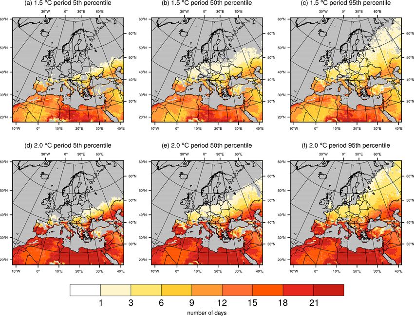
K. Sieck et al.: Weather extremes over Europe under 1.5 and 2.0 ◦ C global warming from HAPPI                                459

et al. (2017) decided to apply their weighting method only        over Europe on a timescale of 10 years is small compared to
to the well-mixed greenhouse gases, because the land-use          the internal variability of a GCM (Sieck and Jacob, 2016).
changes and aerosols show very different spatial patterns and     Each simulation covers a period of 10 years, and as such, ini-
are therefore kept at the 1.5 ◦ C period values.                  tial conditions for the lower boundary need to be in balance
                                                                  with the RCM’s internal climate in order to avoid artificial
2.2   Regional HAPPI simulations
                                                                  drifts in the modelled results. To achieve this, for each driv-
                                                                  ing GCM, the first year of a random GCM member was sim-
In order to create high-resolution climate data for Europe        ulated five times with REMO using initial conditions from
from HAPPI, the RCM REMO has been used for downscal-              the end of the previous run, creating one initial soil state for
ing. REMO is a hydrostatic limited-area model of the atmo-        every ensemble member in one period. This was performed
sphere that has been extensively used and tested in climate       for each of the three periods. Tests showed that this mini-
change studies over Europe (Jacob et al., 2012; Teichmann         mizes drifts in the deep soil climatology compared to initial
et al., 2013; Kotlarski et al., 2014). The simulation domain      conditions taken directly from the GCM (not shown).
follows the CORDEX specification for the standard Euro-              We performed a qualitative analysis of the results com-
pean domain with 0.44◦ horizontal resolution. The Euro-           pared to observations. In general, the performance of
pean CORDEX domain for REMO covers 121 × 129 grid                 the HAPPI ensemble is in line with typical results from
boxes. To exclude the zone where the REMO simulations             the CMIP-type downscaling activities performed in the
are relaxed towards the GCM solutions, a core domain of           CORDEX framework with REMO (see the Supplement for
106 × 103 grid boxes, following the CORDEX definition,            figures and discussion). A list of variables and frequencies
is used for the analyses. In the vertical, 27 levels are used     available from the REMO simulations can be found in the
without nudging except for the boundaries. Boundary condi-        Supplement (see Table S1).
tions are taken from the HAPPI Tier1 experiments (Mitchell
et al., 2017), which are carried out with ECHAM6 in T63
                                                                  2.3     Climate indices
(1.875◦ ) horizontal resolution (Stevens et al., 2013; Lierham-
mer et al., 2017) (100 members per period) and NorESM             To demonstrate how adaptation-relevant information can be
in 1.25◦ × 0.94◦ horizontal resolution (Bentsen et al., 2013)     derived from the HAPPI dataset for two different average
(25 members per period). Both models provide 6-hourly 3-          global temperature targets, four climate indices used in cli-
dimensional data for downscaling. In REMO the same green-         mate impact studies are presented. The extremes are se-
house gas forcings as for the GCMs were used and no land-         lected based on recommended indices developed by the joint
use changes were applied.                                         CCI/CLIVAR/JCOMM Expert Team on Climate Change De-
   SST and sea ice concentrations were taken directly from        tection and Indices (ETCCDI) (Karl et al., 1999; Frich et al.,
the GCM output matching the GCM land–sea mask for                 2002) and other indicators. The selected climate indices are
NorESM. From ECHAM6 only the sea ice concentrations               number of days per year with a daily mean near-surface
were taken. Due to the interpolation procedure for the sea ice    apparent temperature of more than 28 ◦ C (ATG28), annual
extent, it could happen that sea ice was artificially created     maximum 5-day sum of precipitation (RX5day), change in
where no ice conditions were present in the original dataset,     daily precipitation intensity at the 50-year return period
e.g. during summer in the Baltic Sea. ECHAM6 has a mech-          (RI50yr), and consecutive dry days (CDDs) as a measure of
anism that as soon as there is a fraction of sea ice greater      meteorological drought.
than zero, the SST is limited to a maximum of 272.5 K. This          All four climate indices are calculated for each year and
leads to artificial temperature jumps in the SST between ad-      ensemble member. With 100 and 25 members, respectively,
jacent grid boxes as soon as erroneous sea ice appeared in        for 10 years each, the ECHAM6-driven ensembles yield
one of the grid boxes. In order to avoid inheriting this issue,   1000 data points for each grid box and simulation period,
the originally provided SST fields from the HAPPI project         and NorESM-driven ensembles have 250 data points.
were used for the REMO simulations, using ECHAM6 as a
forcing GCM. After testing different temperature and/or sea
                                                                  2.3.1    Apparent temperature
ice fraction thresholds, the authors decided to keep the origi-
nal sea ice maps, because in cases where artificial sea ice was   The ATG28 index is used as an indicator for heat stress,
created the fraction was typically well below 1 % and only in     which is relevant for impacts on human health (Davis et al.,
rare cases reaches up to 4 % (not shown). All other proce-        2016). The apparent temperature is computed using the same
dures would have removed too much sea ice in other seasons        formulation as in Davis et al. (2016):
or led to unrealistic gradients of sea ice fractions. With the
tile approach of REMO, the effect of the artificial sea ice on    AT = −2.653 + 0.994T + 0.0153Td2 ,                          (1)
the averaged near-surface variables is hardly detectable.
   For each GCM member only one REMO simulation was               with AT being the apparent temperature, T the daily mean
carried out, as inter-member variability of an RCM ensemble       near-surface temperature, and Td the daily mean near-surface

https://doi.org/10.5194/esd-12-457-2021                                               Earth Syst. Dynam., 12, 457–468, 2021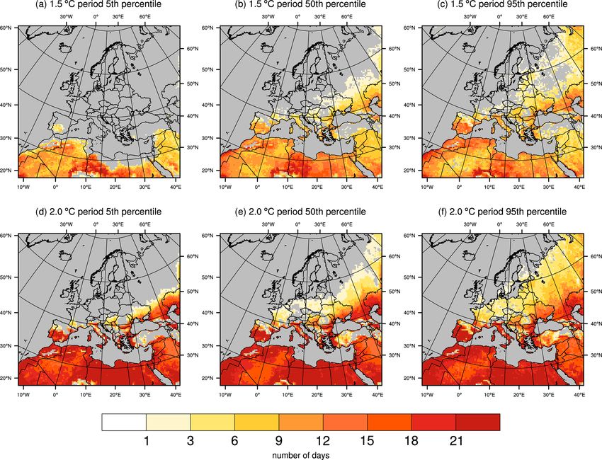
460                       K. Sieck et al.: Weather extremes over Europe under 1.5 and 2.0 ◦ C global warming from HAPPI

dew point temperature. Similar formulations exist in the liter-
ature showing very similar results (see Anderson et al., 2013
for a review). The threshold of 28 ◦ C is based on the defi-
nition of Zhao et al. (2015), who set this limit as the lower
boundary for human heat stress.
   Future changes of ATG28 are analysed by calculating the
differences of the 5th, 50th, and 95th percentiles between
current and projected periods. Only grid boxes with 20 or
more days over 28 ◦ C in the current period were included
in the analysis in order to allow for confidence interval cal-
culations for the calculated percentiles using order statis-
tics. Statistical significance is determined when the calcu-
lated percentile in the 1.5 or 2.0 ◦ C period is outside the per-
centile confidence range of the current period. As ATG28
is temperature-based, changes over the ocean surfaces are
masked out, because they are determined by the prescribed
SST changes to a large extent.

2.3.2   Five-day precipitation sum                                  Figure 1. The European CORDEX domain used by REMO. The
                                                                    outermost black square shows the sponge zone. The PRUDENCE
The annual maximum of the five-day precipitation sum
                                                                    regions are depicted by the boxes with the centred two letter codes:
(RX5day) is used to characterize heavy precipitation events,
                                                                    BI – British Isles, IP – Iberian Peninsula, FR – France, ME – Middle
which can be relevant for flood generation in river basins.         Europe, SC – Scandinavia, AL – Alps, MD – Mediterranean, EA –
The RX5day represents a noisy, i.e. highly spatially and tem-       Eastern Europe.
porally variable parameter. A large ensemble allows for a bet-
ter assessment of the signal-to-noise in extreme precipitation.
   Differences in RX5day are computed by subtracting the            2.3.4    Consecutive dry days
ensemble mean of the current decade from that of the 1.5
and 2.0 ◦ C periods. Statistical significance for RX5day was        Lastly, the consecutive dry days (CDDs), defined as the max-
calculated using a Mann–Whitney U test, and only results            imum number of consecutive days with a daily precipitation
with a significance at the 95 % level are shown.                    amount of less than 1 mm over a region (Karl et al., 1999;
                                                                    Peterson et al., 2001), are calculated for the entire 10-year
2.3.3   Daily precipitation intensity                               period of each ensemble member. The CDD is calculated for
                                                                    each of PRUDENCE regions (Christensen and Christensen,
A change in extreme precipitation directly influences local         2007), illustrated in Fig. 1, because drought indicators are
communities. Such communities have applied design stan-             relevant over large areas, as impacts on water resources oc-
dards for structures to withstand floods with a specified re-       cur at these scales.
turn period. These return standards will no longer be appli-           The significance of changes in the CDD distributions is de-
cable when the extreme value distribution shifts with global        termined using the Mann–Whitney U test with a significance
warming. A Gumbel Type I extreme value distribution is fit-         at the 95 % level. This determines whether samples from the
ted to the annual maxima of daily rainfall amounts. Using           1.5 and 2.0 ◦ C simulations are drawn from a population with
this distribution, an estimate is made of the intensity of rain-    the same distribution as the current period.
fall events associated with a given exceedance probability, in
line with engineering practices. For each ensemble, the daily
rainfall intensity with a 50-year return is computed, hereafter     3     Results
called RI50yr. Information on changes in the rainfall inten-
sity with a 50-year return interval is useful for infrastructure    3.1     Apparent temperature
design and maintenance. For example, road authorities in Eu-
                                                                    Figures 2 and 3 show the changes in ATG28 for the NorESM-
rope typically use between 1- and 10-year return periods for
                                                                    and ECHAM6-driven ensembles, respectively. The grey
assessing effects of rainwater falling on major roads (high-
                                                                    boxes are masked-out areas. On land, they refer to grid boxes
ways) and between 10 and 100 years for rainfall beside the
                                                                    that do not match our criteria of 20 or more occurrences of
road and waters crossing the road (Bless et al., 2018). Dif-
                                                                    ATG28 during the current period. Ocean boxes are masked
ferences in RI50yr between the 1.5 and 2.0 ◦ C simulations
                                                                    out, because any change is very closely related to the pre-
compared and the current period simulations are computed
                                                                    scribed SSTs. In general, the changes are strongest close to
as the relative change in mean daily precipitation intensity.
                                                                    warm ocean areas, especially around the Mediterranean. But

Earth Syst. Dynam., 12, 457–468, 2021                                                   https://doi.org/10.5194/esd-12-457-2021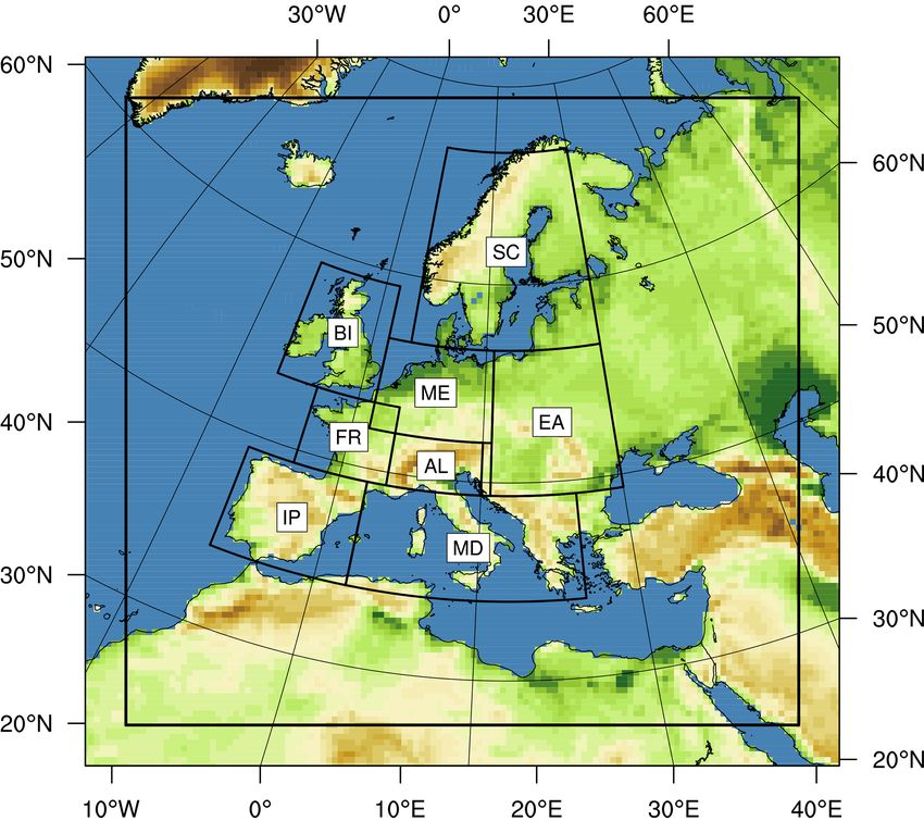
K. Sieck et al.: Weather extremes over Europe under 1.5 and 2.0 ◦ C global warming from HAPPI                                           461

Figure 2. Differences in ATG28 between the current and the 1.5 ◦ C period and (a–c) the 2.0 ◦ C period (d–f) for the NorESM-driven REMO
simulations in number of days. Shown are the differences in the 5th percentile (a, d), median (b, e) and 95th percentile (c, f). Differences
over ocean areas are masked out in grey, as they are closely related to the prescribed SST changes. Masked-out areas over land refer to areas
with fewer than 20 occurrences of ATG28 during the current period.

also the central and eastern parts of Europe show increases              especially important in areas with complex topography such
in ATG28, consistent with the increase in mean temperature               as the Mediterranean region, which is usually only poorly re-
(not shown). The distinct difference between the two warm-               solved in GCM simulations.
ing levels should be noticed. Around the Mediterranean the
increase in ATG28 during the 1.5 ◦ C period is mostly mod-
erate with up to 9 d in the median, whereas changes in the               3.2   Five-day precipitation sum
2.0 ◦ C period reach 18 d and more. This result is consistent
between the ECHAM6- and NorESM-driven ensembles. For                     Figure 4 shows the relative differences of RX5day for the
the northern parts of Spain, on the French Atlantic coast and            REMO ensemble experiments. In general, there is an in-
parts of Eastern Europe, we can note stronger changes for                crease in RX5day over the European part of the domain with
the 95th compared to the 5th percentile. This means that the             stronger signals in the 2.0 ◦ C period compared to the 1.5 ◦ C
shape of the distribution changes towards more highly ex-                period. It can also be seen that the patterns in the ECHAM6-
treme values. For most of the other regions there is only little         driven ensemble are more coherent than the NorESM ensem-
or no change in the shape of the distribution of ATG28. It               ble with larger areas showing a significant change. This is re-
should be noted that the spatial resolution of the simulations           lated to the difference in ensemble size between ECHAM6-
allows one to show the lower level of warming in mountain-               and NorESM-driven simulations and underlines the neces-
ous areas compared to coastal areas, e.g. over Italy. This is            sity for a large ensemble to achieve proper signal-to-noise
                                                                         ratios when looking at the difference in regional changes un-

https://doi.org/10.5194/esd-12-457-2021                                                       Earth Syst. Dynam., 12, 457–468, 2021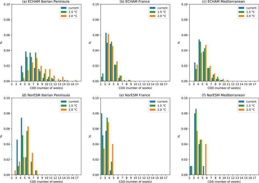
462                      K. Sieck et al.: Weather extremes over Europe under 1.5 and 2.0 ◦ C global warming from HAPPI

Figure 3. Same as Fig. 2, but for the ECHAM6-driven REMO simulations.

der small GMT increases in highly variable quantities such        3.3   Daily rainfall intensity, 50-year return period
as precipitation extremes. Tests with a randomly picked 25-
                                                                  Figure 5 shows spatial differences in the 50-year return
member ensemble from the ECHAM6-driven simulations
                                                                  period of daily rainfall intensity (RI50yr) across Europe.
showed a similarly noisy pattern as the NorESM-driven runs
                                                                  In both the NorESM- and ECHAM6-driven ensembles, a
(see Supplement).
                                                                  greater increase in the rainfall intensity is found in the 2.0 ◦ C
   Apart from artificial effects due to the boundary condi-
                                                                  simulations compared to 1.5 ◦ C. ECHAM6-driven simula-
tions, the strongest signal within the core domain appears
                                                                  tions clearly show increases in RI50yr of up to 20 % over
over the Baltic Sea, with an increase of up to 15 % in RX5day
                                                                  continental Europe. The estimated changes in rainfall inten-
under a 2.0 ◦ C increase in GMT. This result is consistent be-
                                                                  sity in the NorESM-driven simulations appear to be more ex-
tween both ensembles. A similar increase can be seen over
                                                                  treme, but these simulations are also noisier as they are based
the Adriatic Sea but is not so pronounced in the ECHAM6-
                                                                  on fewer ensemble members.
driven ensemble. This might be related to feedbacks from
insufficiently resolved SSTs, because the GCMs usually do
not resolve these small sub-basins well. In the case of the       3.4   Consecutive dry days
Adriatic Sea, where precipitation amounts are highly sensi-       In this section, changes in the distributions of consecutive
tive to changes in local SST (e.g. Stocci and Davolio, 2016),     dry days (CDDs) for the 1.5 and 2.0 ◦ C periods compared
this can lead to biases in heavy precipitation amounts.           to the current period are presented. To distinguish whether
                                                                  these changes in the distributions are statistically significant,
                                                                  we employ the Mann–Whitney U test. When the resulting
                                                                  p values of the test are less than or equal to 0.05, the null

Earth Syst. Dynam., 12, 457–468, 2021                                                https://doi.org/10.5194/esd-12-457-2021
K. Sieck et al.: Weather extremes over Europe under 1.5 and 2.0 ◦ C global warming from HAPPI 463 Figure 4. Relative difference of RX5day (in percent) between current and the 1.5 ◦ C period and (a, b) the 2.0 ◦ C period (c, d) for the ECHAM6 with 100 members (a, c) and NorESM with 25 members (b, d) driven REMO simulations. Grey shading shows areas with non- significant changes on the 95 % significance level. hypothesis is rejected indicating the distributions differ. The have changes in CDD distributions under 1.5 and 2.0 ◦ C that p values for each of the PRUDENCE regions (Christensen are statistically indistinguishable from the current period (Ta- and Christensen, 2007; see Fig. 1) are presented in Table 1. ble 1). One can deduce that region 2 will likely have longer Bold numbers in Table 1 indicate that the distributions are drought periods than experienced before compared to regions significantly different. 6 and 8. Interestingly, for region 7, the Mediterranean, the We begin by looking at three regions where the Mann– CDD distributions of the ECHAM6 and NorESM ensem- Whitney U test provided consistent results across the ensem- bles of 1.5 ◦ C do not differ statistically from the current pe- bles. In region 2, the Iberian Peninsula, the CDD distribu- riod, yet both ensembles show a statistically different distri- tions in both the 1.5 and 2.0 ◦ C simulations differ statistically bution at 2.0 ◦ C. Thus, one can conclude for region 7, accord- compared to the simulations for the current period. Over this ing to these simulations, a lower target of 1.5 ◦ C increase in region, one can see an increase in the duration of the longest GMT could reduce the length of the maximum number of dry period, and the probability of having a CDD, which ex- dry days in this region, compared to a 2.0 ◦ C target. In re- ceeds 9 weeks, is greater in the warmer scenarios (Fig. 6). gion 3, France, the results of the two ensembles differ. The In contrast, regions 6 and 8, the Alps and Eastern Europe, ECHAM6 simulations suggest that there is no difference in https://doi.org/10.5194/esd-12-457-2021 Earth Syst. Dynam., 12, 457–468, 2021
464                         K. Sieck et al.: Weather extremes over Europe under 1.5 and 2.0 ◦ C global warming from HAPPI

Figure 5. Relative difference of RI50yr (in percent) between current and the 1.5 ◦ C period and (a, b) the 2.0 ◦ C period (c, d) for ECHAM6
with 100 members (a, c) and the NorESM with 25 members (b, d) driven REMO simulations.

Table 1. Mann–Whitney U test p values for distributions of consecutive dry days (CDDs) for the ECHAM6- and NorESM-driven ensembles
for different PRUDENCE regions (for locations see Fig. 1). Bold values indicate statistically significant differences.

                               PRUDENCE region                 ECHAM6                        NorESM
                                                       Current vs. Current vs.      Current vs. Current vs.
                                                         1.5 ◦ C     2.0 ◦ C          1.5 ◦ C      2.0 ◦ C
                               1. British Isles           0.270         0.035          0.024          0.053
                               2. Iberian Peninsula       0.036         0.000          0.000          0.000
                               3. France                  0.391         0.230          0.015          0.002
                               4. Middle Europe           0.077         0.015          0.363          0.212
                               5. Scandinavia             0.238         0.356          0.046          0.081
                               6. Alps                    0.333         0.105          0.378          0.355
                               7. Mediterranean           0.069         0.036          0.348          0.021
                               8. Eastern Europe          0.325         0.465          0.419          0.385

Earth Syst. Dynam., 12, 457–468, 2021                                                          https://doi.org/10.5194/esd-12-457-2021
K. Sieck et al.: Weather extremes over Europe under 1.5 and 2.0 ◦ C global warming from HAPPI 465
Figure 6. Duration of drought events in three PRUDENCE regions (Iberian Peninsula, France, and the Mediterranean) under 1.5 and 2.0◦
global warming for the ECHAM-driven (a–c) and NorESM-driven (d–f) ensembles. For significance see Table 1.
CDD distributions between the warmer climate compared to a 0.5 ◦ C higher global mean warming can have consider-
the current period, whereas the NorESM simulations find the able consequences for human health. This is especially true
warmer climate has a distinctly different CDD distribution around the Mediterranean, where changes towards hotter and
compared to the current period. more humid conditions along the coasts can have negative
impacts on the population and may increase mortality due
to heat stress. The tourism sector may also be negatively
4 Discussion and conclusions affected by hotter and more humid conditions. Robust esti-
mates of percentiles and changes in percentiles can be de-
A unique climate dataset has been presented that enables rived from the large ensemble. Some regions show a change
the quantification of differences between a 1.5 and 2.0 ◦ C of the shape in distribution of ATG28 towards higher extreme
warmer world compared to pre-industrial times on a re- values. These findings are not directly comparable to earlier
gional level. This dataset can support climate change im- studies but are in line with studies on extreme temperatures
pact studies on the regional scale with physically consis- under 1.5 and 2.0 ◦ C warming (e.g. Schleussner et al., 2016;
tent data, which is often not possible to achieve with other Sanderson et al., 2017; Suarez-Gutierrez et al., 2018).
methods than dynamical downscaling. The use of a large en- RX5day shows a general increase over Europe which is
semble (100 × 10 years) compared to alternative datasets for more pronounced under higher global mean warming. More
analysing changes under different temperature targets is es- coherent spatial patterns with larger areas showing signif-
pecially beneficial to assess changes in highly variable mete- icant changes result from the larger ensemble driven by
orological parameters, such as extreme temperature and pre- ECHAM6 (100 members) compared to the smaller ensem-
cipitation. In general, the 100 members driven by ECHAM6 ble driven by NorESM (25 members) and also compared to a
provide information of statistically significant changes over smaller sub-ensemble driven by ECHAM6, which underlines
relatively large and spatially homogeneous areas. In compar- the need for large ensemble size to reliably detect changes in
ison, the 25-member ensemble driven by NorESM shows a highly variable quantities such as precipitation extremes. Our
much noisier spatial pattern which lowers confidence in the results for RX5day are in line with earlier findings by King
projected changes. and Karoly (2017), who investigate RX1day for Europe un-
The significant differences in apparent temperature der 1.5 and 2.0 ◦ C warming. They find that heaviest rainfall
ATG28 under different global mean warming level show that
https://doi.org/10.5194/esd-12-457-2021 Earth Syst. Dynam., 12, 457–468, 2021466 K. Sieck et al.: Weather extremes over Europe under 1.5 and 2.0 ◦ C global warming from HAPPI
events would be more likely under 2 ◦ C warming compared The current dataset was created using the only two GCMs
to 1.5 ◦ C. available at the time for downscaling, one with a reduced
With regard to the change in the daily rainfall intensity at number of ensemble members. As more GCM ensembles
the 50-year return period (RI50yr), a greater increase in rain- become available for downscaling in the future, it will al-
fall intensity was found in the 2.0 ◦ C warmer world. Given low for new studies which can provide more robust estimates
these changes, information can be derived for local com- of inter-model variability/uncertainty. Nevertheless, there is
munities, which must consider changes in rainfall intensity currently a unique dataset targeted to the Paris agreement
when designing hydraulic and water resource infrastructures, goals available for further analysis. A comparison with al-
as well as transportation infrastructure, including highways ternative methods for extracting the warming level is lacking
and bridges. Cost considerations associated with increasing and should be done in future studies.
rain intensity demands can be computed for upcoming design
projects to ensure investments remain beneficial. The HAPPI
dataset can be used to calculate other return periods, catering Data availability. The data are stored in the internal DKRZ tape
to the demands of individual sectors. archive. Due to the number of data, it is has not been possible to
Robust high and low percentile changes for precipitation make them available via a publicly accessible data portal. A list of
are still difficult to distil on a grid box level from the data available variables in netCDF format is given in the Supplement,
and data requests can be sent to happi-data@hereon.de.
because of the high variability of precipitation extremes, but
methods such as spatial aggregation might help to achieve
robust signals on larger spatial scale.
Supplement. The supplement related to this article is available
The changes to CDD distributions show that Spain would
online at: https://doi.org/10.5194/esd-12-457-2021-supplement.
experience longer droughts in the future compared to the cur-
rent period, even with a 1.5 ◦ C increase in GMT. For Italy,
drought conditions associated with the 1.5 ◦ C simulations Author contributions. KS and DJ designed the study. KS per-
show non-significant changes, yet those associated with the formed the regional climate model simulations. KS and CN did
2.0 ◦ C simulations are significantly different to the current the analysis of the climate indices and created the plots. KS, CN,
period, thus showing possible consequences of exceeding the LMB and DR wrote the initial draft paper. All authors contributed
1.5 ◦ C GMT target of the Paris Agreement. with discussions and revisions.
The relatively coarse resolution of 0.44◦ for a dynamical
downscaling study over Europe is a compromise between
model complexity, resolution and ensemble size. In particu- Competing interests. The authors declare that they have no con-
lar, the coarse driving data of the ECHAM6 model with T63 flict of interest.
(1.875◦ ) horizontal resolution do not allow for direct down-
scaling to a much higher resolution, such as 0.22◦ , without
having a large spatial spin-up of small-scale features inside Acknowledgements. The authors thank the three anonymous ref-
the domain (see e.g. Matte et al., 2017). We do not expect erees and Laura Suarez-Gutierrez for providing comments that
helped to improve this paper. We also thank the German Climate
fundamental qualitative changes to our findings at a resolu-
Computing Center (DKRZ) for supplying computing time and the
tion of 0.22◦ , except where regional mesoscale features play
HAPPI consortium for providing the boundary conditions for the
an important role. downscaling. We acknowledge the E-OBS dataset from the EU-FP6
As pointed out by Fischer et al. (2018), data from AMIP project ENSEMBLES (http://ensembles-eu.metoffice.com, last ac-
ensembles such as HAPPI have to be used with caution. In cess: 23 April 2021) and the data providers in the ECA & D project
regions and on timescales where oceanic variability plays an (http://www.ecad.eu, last access: 1 May 2018). The authors thank
important role, results from AMIP ensembles tend to over- their co-workers for the valuable discussions. This work is part of
estimate extremes and often show overconfidence with a too the research project HAPPI-DE supported by the German Federal
high a significance of the results. For Europe, this effect is Ministry of Education and Research (BMBF) under grant number
especially important on seasonal or longer timescales. For 01LS1613C. It was also supported by the Digital Earth project of
shorter-term events such as daily extremes, AMIP ensembles the Helmholtz Association, funding code ZT-0025.
compare equally well with other methods in the mid and high
latitudes, because they are dominated by atmospheric vari-
Financial support. This research has been supported by the Bun-
ability.
desministerium für Bildung und Forschung (grant no. 01LS1613C).
The results for most of the indices presented should not
be affected because they specifically target short timescale The article processing charges for this open-access
extremes. In the case of CDD it depends on the region inves- publication were covered by a Research
tigated. In some regions CDD comes close to or even exceeds Centre of the Helmholtz Association.
an entire season. In these cases, one should confirm any find-
ings using other sources, e.g. ensembles of coupled GCMs.
Earth Syst. Dynam., 12, 457–468, 2021 https://doi.org/10.5194/esd-12-457-2021K. Sieck et al.: Weather extremes over Europe under 1.5 and 2.0 ◦ C global warming from HAPPI 467
Review statement. This paper was edited by Gabriele Messori Gutowski Jr., W. J., Giorgi, F., Timbal, B., Frigon, A., Jacob, D.,
and reviewed by three anonymous referees. Kang, H.-S., Raghavan, K., Lee, B., Lennard, C., Nikulin, G.,
O’Rourke, E., Rixen, M., Solman, S., Stephenson, T., and Tan-
gang, F.: WCRP COordinated Regional Downscaling EXperi-
ment (CORDEX): a diagnostic MIP for CMIP6, Geosci. Model
References Dev., 9, 4087–4095, https://doi.org/10.5194/gmd-9-4087-2016,
2016.
Anderson, G. B., Bell, M. L., and Peng, R. D.: Methods to calcu- He, J. and Soden, B. J.: The Impact of SST Biases on Projec-
late the heat index as an exposure metric in environmental health tions of Anthropogenic Climate Change: A Greater Role for
research, Environ. Health Persp., 121, 1111–1119, 2013. Atmosphere-only Models?, Geophys. Res. Lett., 43, 7745–7750,
Bentsen, M., Bethke, I., Debernard, J. B., Iversen, T., Kirkevåg, A., 2016.
Seland, Ø., Drange, H., Roelandt, C., Seierstad, I. A., Hoose, C., IPCC: Global Warming of 1.5 ◦ C. An IPCC Special Report on the
and Kristjánsson, J. E.: The Norwegian Earth System Model, impacts of global warming of 1.5 ◦ C above pre-industrial lev-
NorESM1-M – Part 1: Description and basic evaluation els and related global greenhouse gas emission pathways, in the
of the physical climate, Geosci. Model Dev., 6, 687–720, context of strengthening the global response to the threat of cli-
https://doi.org/10.5194/gmd-6-687-2013, 2013. mate change, sustainable development, and efforts to eradicate
Bles, T., De Lange, D., Foucher, L., Axelsen, C., Leahy, C., and poverty, edited by: Masson-Delmotte, V., Zhai, P., Pörtner, H. O.,
Rooney, J. P.: Water management for road authorities in the Roberts, D., Skea, J., Shukla, P. R., Pirani, A., Moufouma-
face of climate Change: Country Comparison Report, Con- Okia, W., Péan, C., Pidcock, R., Connors, S., Matthews, J. B. R.,
ference of European Directors of Roads (CEDR), Brussels, Chen, Y., Zhou, X., Gomis, M. I., Lonnoy, E., Maycock, T., Tig-
available at: https://www.cedr.eu/strategic-plan-tasks/research/ nor, M., and Waterfield, T., Intergovernmental Panel on Climate
cedr-call-2015/call-2015-climate-change-desk-road/ (last ac- Change, World Meteorological Organization, Geneva, Switzer-
cess: 13 December 2019), 2018. land, 2018.
Christensen, J. H. and Christensen, O. B.: A summary of the PRU- Jacob, D., Elizalde, A., Haensler, A., Hagemann, S., Kumar, P.,
DENCE model projections of changes in European climate by Podzun, R., Rechid, D., Remedio, A. R., Saeed, F., Sieck, K.,
the end of this century, Climatic Change, 81, 7–30, 2007. Teichmann, C., and Wilhelm, C.: Assessing the transferability of
Davis, R. E., McGregor, G. R., and Eneld, K. B.: Humidity: A re- the regional climate model REMO to different coordinated re-
view and primer on atmospheric moisture and human health, En- gional climate downscaling experiment (CORDEX) regions, At-
viron. Res., 144, 106–116, 2016. mosphere, 3, 181–199, 2012.
Deser, C., Phillips, A. S., Alexander, M. A., and Smoliak, B. V.: Jacob, D., Petersen, J., Eggert, B., Alias, A., Christensen, O. B.,
Projecting North American climate over the next 50 years: Un- Bouwer, L. M., Braun, A., Colette, A., Déqué, M.,
certainty due to internal variability, J. Climate, 27, 2271–2296, Georgievski, G., Georgopoulou, E., Gobiet, A., Menut, L.,
https://doi.org/10.1175/JCLI-D-13-00451.1, 2014. Nikulin, G., Haensler, A., Hempelmann, N., Jones, C.,
Eyring, V., Bony, S., Meehl, G. A., Senior, C. A., Stevens, B., Keuler, K., Kovats, S., Kröner, N., Kotlarski, S., Kriegs-
Stouffer, R. J., and Taylor, K. E.: Overview of the Coupled mann, A., Martin, E., van Meijgaard, E., Moseley, C., Pfeifer, S.,
Model Intercomparison Project Phase 6 (CMIP6) experimen- Preuschmann, S., Radermacher, C., Radtke, K., Rechid, D.,
tal design and organization, Geosci. Model Dev., 9, 1937–1958, Rounsevell, M., Samuelsson, P., Somot, S., Soussana, J.-F.,
https://doi.org/10.5194/gmd-9-1937-2016, 2016. Teichmann, C., Valentini, R., Vautard, R., Weber, B., and
Fischer, E. M., Beyerle, U., Schleussner, C. F., King, A. D., and Yiou, P.: Euro-CORDEX: New high-resolution climate change
Knutti, R.: Biased Estimates of Changes in Climate Extremes projections for European impact research, Reg. Environ. Change,
From Prescribed SST Simulations, Geophys. Res. Lett., 45, 14, 563–578, https://doi.org/10.1007/s10113-013-0499-2, 2014.
8500–8509, 2018. Jacob, D., Kotova, L., Teichmann, C., Sobolowski, S. P., Vau-
Frich, P., Alexander, L. V., Della-Marta, P., Gleason, B., Hay- tard, R., Donnelly, C., Koutroulis, A. G., Grillakis, M. G., Tsa-
lock, M., Klein Tank, A. M. G., and Peterson, T.: Observed co- nis, I. K., Damm, A., Sakalli, A., and Van Vliet, M. T. H.: Climate
herent changes un climatic extremes during the second half of impacts in Europe under +1.5 ◦ C global warming, Earths Future,
the twentieth century, Clim. Res., 18, 193–212, 2002. 6, 264–285, https://doi.org/10.1002/2017EF000710, 2018.
Gates, W. L.: AMIP: The Atmospheric Model In- Karl, T. R., Nicholls, N., and Ghazi, A.: CLIVAR/GCOS/WMO
tercomparison Project, B. Am. Meteorol. Soc., workshop on indices and indicators for climate extremes Work-
73, 1962–1970, https://doi.org/10.1175/1520- shop summary, Climatic Change, 42, 3–7, 1999.
0477(1992)0732.0.CO;2, 1992. King, A. D. and Karoly, D. J.: Climate extremes in Europe at 1.5 and
Giorgi, F. and Gutowski, W. J.: Regional dynamical downscal- 2 degrees of global warming, Environ. Res. Lett., 12, 114031,
ing and the CORDEX initiative, Annu. Rev. Env. Resour., https://doi.org/10.1088/1748-9326/aa8e2c, 2017.
40, 467–490, https://doi.org/10.1146/annurev-environ-102014- Kotlarski, S., Keuler, K., Christensen, O. B., Colette, A., Déqué, M.,
021217, 2015. Gobiet, A., Goergen, K., Jacob, D., Lüthi, D., van Meijgaard, E.,
Giorgi, F. and Jones, C. A. G.: Addressing climate information Nikulin, G., Schär, C., Teichmann, C., Vautard, R., Warrach-
needs at the regional level: The CORDEX framework, WMO Sagi, K., and Wulfmeyer, V.: Regional climate modeling on
Bulletin, 58, 175–183, 2009. European scales: a joint standard evaluation of the EURO-
Goldstein, A., Turner, W. R., Gladstone, J., and Hole, D. G.: The CORDEX RCM ensemble, Geosci. Model Dev., 7, 1297–1333,
private sector’s climate change risk and adaptation blind spots, https://doi.org/10.5194/gmd-7-1297-2014, 2014.
Nat. Clim. Change, 9, 18–25, 2018.
https://doi.org/10.5194/esd-12-457-2021 Earth Syst. Dynam., 12, 457–468, 2021468 K. Sieck et al.: Weather extremes over Europe under 1.5 and 2.0 ◦ C global warming from HAPPI Leduc, M., Mailhot, A., Frigon, A., Martel, J., Ludwig, R., Briet- Sieck, K. and Jacob, D.: Influence of the boundary forcing on the zke, G. B., Giguère, M., Brissette, F., Turcotte, R., Braun, M., internal variability of a regional climate model, Am. J. Clim. and Scinocca, J.: The ClimEx Project: A 50-Member ensemble Change, 5, 373–382, https://doi.org/10.4236/ajcc.2016.53028, of climate change projections at 12-km resolution over Europe 2016. and northeastern North America with the Canadian Regional Cli- Stevens, B., Giorgetta, M., Esch, M., Mauritsen, T., Crueger, T., mate Model (CRCM5), J. Appl. Meteorol. Clim., 58, 663–693, Rast, S., Salzmann, M., Schmidt, H., Bader, J., Block, K., https://doi.org/10.1175/JAMC-D-18-0021.1, 2019. Brokopf, R., Fast, I., Kinne, S., Kornblueh, L., Lohmann, U., Pin- Lierhammer, L., Mauritsen, T., Legutke, S., Esch, M., cus, R., Reichler, T., and Roeckner, E.: Atmospheric component Wieners, K. H., and Saeed, F.: Simulations of HAPPI of the MPI-M Earth System Model: ECHAM6, J. Adv. Model (Half a degree Additional warming, Prognosis and Pro- Earth Sy., 5, 146–172, https://doi.org/10.1002/jame.20015, 2013. jected Impacts) Tier-1 experiments based on the ECHAM6.3 Stocchi, P. and Davolio, S.: Intense air-sea exchange and heavy rain- atmospheric model of the Max Planck Institute for Meteo- fall: impact of the northern Adriatic SST, Adv. Sci. Res., 13, 7– rology (MPI-M), World Data Center for Climate (WDCC) at 12, https://doi.org/10.5194/asr-13-7-2016, 2016. DKRZ, https://doi.org/10.1594/WDCC/HAPPI-MIP-global- Suarez-Gutierrez, L., Li, C., Müller, W. A., and Marotzke, J.: In- ECHAM6.3, 2017. ternal variability in European summer temperatures at 1.5 ◦ C Matte, D., Laprise, R., Thériault, J. M., and Lucas-Picher, P.: Spa- and 2 ◦ C of global warming, Environ. Res. Lett., 13, 064026, tial spin-up of fine scales in a regional climate model simulation https://doi.org/10.1088/1748-9326/aaba58, 2018. driven by low-resolution boundary conditions, Clim. Dynam., Taylor, K. E., Stouffer, R. J., and Meehl, G. A.: An overview of 49, 563–574, 2017. CMIP5 and the experiment design, B. Am. Meteorol. Soc., 93, Meinshausen, M., Nicholls, Z. R. J., Lewis, J., Gidden, M. J., 485–498, https://doi.org/10.1175/BAMS-D-11-00094.1, 2012. Vogel, E., Freund, M., Beyerle, U., Gessner, C., Nauels, A., Teichmann, C., Eggert, B., Elizalde, A., Haensler, A., Jacob, D., Bauer, N., Canadell, J. G., Daniel, J. S., John, A., Krum- Kumar, P., Moseley, C., Pfeifer, S., Rechid, D., Remedio, A. R., mel, P. B., Luderer, G., Meinshausen, N., Montzka, S. A., Ries, H., Petersen, J., Preuschmann, S., Raub, T., Saeed, F., Rayner, P. J., Reimann, S., Smith, S. J., van den Berg, M., Sieck, K., and Weber, T.: How does a regional climate model Velders, G. J. M., Vollmer, M. K., and Wang, R. H. J.: The modify the projected climate change signal of the driving GCM: shared socio-economic pathway (SSP) greenhouse gas concen- A study over different CORDEX regions using REMO, Atmo- trations and their extensions to 2500, Geosci. Model Dev., 13, sphere, 4, 214–236, 2013. 3571–3605, https://doi.org/10.5194/gmd-13-3571-2020, 2020. UNFCCC: Paris Agreement, United Nations Framework Mitchell, D., James, R., Forster, P. M., Betts, R. A., Sh- Convention on Climate Change, Bonn, available at: iogama, H., and Allen, M.: Realizing the impacts of a https://unfccc.int/files/essential_background/convention/ 1.5 ◦ C warmer world, Nat. Clim. Change, 6, 735–267, application/pdf/english_paris_agreement.pdf (last access: https://doi.org/10.1038/nclimate3055, 2016. 23 April 2021), 2015. Mitchell, D., AchutaRao, K., Allen, M., Bethke, I., Beyerle, U., Van Vuuren, D. P., Edmonds, J., Kainuma, M., Riahi, K., Thom- Ciavarella, A., Forster, P. M., Fuglestvedt, J., Gillett, N., son, A., Hibbard, K., Hurtt, G. C., Kram, T., Krey, V., Haustein, K., Ingram, W., Iversen, T., Kharin, V., Klingaman, N., Lamarque, J.-F., Masui, T., Meinshausen, M., Nakicenovic, N., Massey, N., Fischer, E., Schleussner, C.-F., Scinocca, J., Se- Smith, S. J., and Rose, S. K.: The representative concen- land, Ø., Shiogama, H., Shuckburgh, E., Sparrow, S., Stone, D., tration pathways: An overview, Climatic Change, 109, 5–31, Uhe, P., Wallom, D., Wehner, M., and Zaaboul, R.: Half a degree https://doi.org/10.1007/s10584-011-0148-z, 2011. additional warming, prognosis and projected impacts (HAPPI): Vautard, R., Gobiet, A., Sobolowski, S., Kjellström, E., Stege- background and experimental design, Geosci. Model Dev., 10, huis, A., Watkiss, P., Mendlik, T., Landgren, O., Nikulin, G., 571–583, https://doi.org/10.5194/gmd-10-571-2017, 2017. Teichmann, C., and Jacob, D.: The European climate un- Peterson, T. C., Folland, C., Gruza, G., Hogg, W., Mokssit, A., and der a 2 ◦ C global warming, Environ. Res. Lett., 9, 034006, Plummer, N.: Report on the Activities of the Working Group on https://doi.org/10.1088/1748-9326/9/3/034006, 2014. Climate Change Detection and Related Rapporteurs 1998–2001. Zhao, Y., Ducharne, A., Sultan, B., Braconnot, P., and Vau- Report WCDMP-47, WMO-TD 1071, World Meteorological Or- tard, R.: Estimating heat stress from climate-based indicators: ganization, Geneva, 2001. present-day biases and future spreads in the CMIP5 global Sanderson, B. M., Xu, Y., Tebaldi, C., Wehner, M., O’Neill, B., climate model ensemble, Environ. Res. Lett., 10, 084013, Jahn, A., Pendergrass, A. G., Lehner, F., Strand, W. G., Lin, L., https://doi.org/10.1088/1748-9326/10/8/084013, 2015. Knutti, R., and Lamarque, J. F.: Community climate simulations to assess avoided impacts in 1.5 and 2 ◦ C futures, Earth Syst. Dy- nam., 8, 827–847, https://doi.org/10.5194/esd-8-827-2017, 2017. Schleussner, C.-F., Lissner, T. K., Fischer, E. M., Wohland, J., Perrette, M., Golly, A., Rogelj, J., Childers, K., Schewe, J., Frieler, K., Mengel, M., Hare, W., and Schaeffer, M.: Differen- tial climate impacts for policy-relevant limits to global warming: the case of 1.5 ◦ C and 2 ◦ C, Earth Syst. Dynam., 7, 327–351, https://doi.org/10.5194/esd-7-327-2016, 2016. Earth Syst. Dynam., 12, 457–468, 2021 https://doi.org/10.5194/esd-12-457-2021
You can also read