A global gridded (0.1 0.1 ) inventory of methane emissions from oil, gas, and coal exploitation based on national reports to the United Nations ...
←
→
Page content transcription
If your browser does not render page correctly, please read the page content below
Earth Syst. Sci. Data, 12, 563–575, 2020
https://doi.org/10.5194/essd-12-563-2020
© Author(s) 2020. This work is distributed under
the Creative Commons Attribution 4.0 License.

            A global gridded (0.1◦ × 0.1◦ ) inventory of methane
           emissions from oil, gas, and coal exploitation based
           on national reports to the United Nations Framework
                      Convention on Climate Change
        Tia R. Scarpelli1 , Daniel J. Jacob1 , Joannes D. Maasakkers1 , Melissa P. Sulprizio1 , Jian-Xiong Sheng1 ,
                    Kelly Rose2 , Lucy Romeo2 , John R. Worden3 , and Greet Janssens-Maenhout4
                                      1 Harvard  University, Cambridge, MA 02138, USA
               2 U.S.  Department of Energy, National Energy Technology Laboratory, Albany, OR 97321, USA
                   3 Jet Propulsion Laboratory, California Institute of Technology, Pasadena, CA 91109, USA
                                    4 European Commission Joint Research Centre, Ispra, Italy

                                Correspondence: Tia R. Scarpelli (tscarpelli@g.harvard.edu)

                                  Received: 20 July 2019 – Discussion started: 17 September 2019
                         Revised: 2 February 2020 – Accepted: 4 February 2020 – Published: 11 March 2020

       Abstract. Individual countries report national emissions of methane, a potent greenhouse gas, in accordance
       with the United Nations Framework Convention on Climate Change (UNFCCC). We present a global inven-
       tory of methane emissions from oil, gas, and coal exploitation that spatially allocates the national emissions
       reported to the UNFCCC (Scarpelli et al., 2019). Our inventory is at 0.1◦ × 0.1◦ resolution and resolves the
       subsectors of oil and gas exploitation, from upstream to downstream, and the different emission processes (leak-
       age, venting, flaring). Global emissions for 2016 are 41.5 Tg a−1 for oil, 24.4 Tg a−1 for gas, and 31.3 Tg a−1
       for coal. An array of databases is used to spatially allocate national emissions to infrastructure, including wells,
       pipelines, oil refineries, gas processing plants, gas compressor stations, gas storage facilities, and coal mines.
       Gridded error estimates are provided in normal and lognormal forms based on emission factor uncertainties
       from the IPCC. Our inventory shows large differences with the EDGAR v4.3.2 global gridded inventory both
       at the national scale and in finer-scale spatial allocation. It shows good agreement with the gridded version of
       the United Kingdom’s National Atmospheric Emissions Inventory (NAEI). There are significant errors on the
       0.1◦ × 0.1◦ grid associated with the location and magnitude of large point sources, but these are smoothed out
       when averaging the inventory over a coarser grid. Use of our inventory as prior estimate in inverse analyses of at-
       mospheric methane observations allows investigation of individual subsector contributions and can serve policy
       needs by evaluating the national emissions totals reported to the UNFCCC. Gridded data sets can be accessed at
       https://doi.org/10.7910/DVN/HH4EUM (Scarpelli et al., 2019).

1   Introduction                                                   wastewater treatment. Individual countries must estimate
                                                                   and report their anthropogenic methane emissions by source
Methane is the second most important anthropogenic green-          to the United Nations in accordance with the United Na-
house gas after CO2 , with an emission-based radiative forc-       tions Framework Convention on Climate Change (UNFCCC,
ing of 1.0 W m−2 since pre-industrial times, as compared           1992). These estimates rely on emission factors (amount
to 1.7 W m−2 for CO2 (Myhre et al., 2013). Major anthro-           emitted per unit of activity) that can vary considerably be-
pogenic sources of methane include the oil and gas indus-          tween countries in particular for oil and gas (Larsen et al.,
try, coal mining, livestock, rice cultivation, landfills, and      2015). This variation may reflect differences in infrastructure

Published by Copernicus Publications.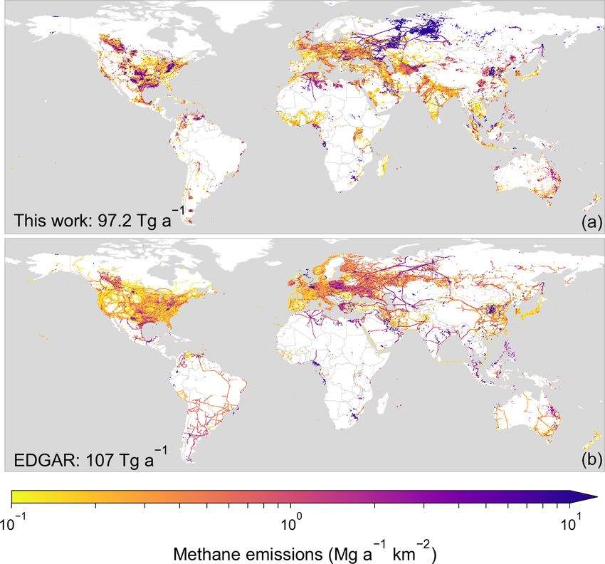
564                                                       T. R. Scarpelli et al.: A global inventory of fuel exploitation methane

between countries but also large uncertainties (Allen et al.,      ture (GOGI) inventory and geodatabase (Rose et al., 2018;
2015; Brantley et al., 2014; Mitchell et al., 2015; Omara et       Sabbatino et al., 2017), and other sources. National emissions
al., 2016; Robertson et al., 2017), including a possible under-    from coal mining are distributed according to mine locations
accounting of abnormally high emitters (Duren et al., 2019;        from EDGAR v4.3.2. We present results for 2016, which is
Zavala-Araiza et al., 2015).                                       the most recent year available from the UNFCCC, but our
   Top-down inverse analyses of atmospheric methane obser-         method is readily adaptable to other years.
vations can provide a check on the national emission inven-
tories (Jacob et al., 2016), but they require prior information
                                                                   2     Data and methods
on the spatial distribution of emissions within the country.
This information is not available from the UNFCCC reports.         2.1     National emissions data
The EDGAR global emission inventory with 0.1◦ ×0.1◦ grid-
ded resolution (European Commission, 2011, 2017) has been          Figure 1 gives a flow chart of the emission processes from oil,
used extensively as prior estimate for methane emissions in        gas, and coal exploitation as resolved in our inventory. The
inverse analyses. EDGAR prioritizes the use of a consis-           emissions characterized here correspond to the IPCC (2006)
tent methodology between countries for emissions estimates,        category “fugitive emissions from fuels” (category code 1B).
including the use of IPCC Tier 1 methods (IPCC, 2006),             Here and elsewhere we refer to “sectors” as oil, gas, or coal.
and then spatially distributes emissions using proxy data like     We refer to “subsectors” as the separate activities for each
satellite observations of gas flaring (Janssens-Maenhout et        sector resolved in Fig. 1, e.g., “gas production”. The subsec-
al., 2019). However, its oil and gas emissions show large dif-     tors were chosen to match UNFCCC reporting as much as
ferences compared to inventories that utilize more detailed        possible. We refer to “processes” as the means of emission,
data specific to a country or region (Jeong et al., 2014; Lyon     which can be leakage, venting, or flaring. Leakage emissions
et al., 2015; Maasakkers et al., 2016; Sheng et al., 2017). The    include all unintended emissions, such as from equipment
latest public version, EDGAR v5.0 (Crippa et al., 2019; Eu-        leaks, evaporation losses, and accidental releases. Coal emis-
ropean Commission, 2019), provides separate gridded prod-          sions are lumped together, including contributions from sur-
ucts for oil, gas, and coal exploitation emissions for each        face and underground mines during mining and post-mining
year from 1970 to 2015 but with no further subsector break-        activities (IPCC, 2006), without further partitioning because
down. Some other regional and global multispecies emis-            the emissions are mainly at the locations of the mines. We
sion inventories also include methane but have coarse spa-         create a separate gridded inventory file for each sector, sub-
tial and/or sectoral resolution, such as CEDS (Hoesly et al.,      sector, and process as specified by the individual boxes of
2018), REAS (Kurokawa et al., 2013), or GAINS (Höglund-            Fig. 1. The subsectors reported by countries to the UNFCCC
Isaksson, 2012). Gridded emission inventories for the oil,         vary, so our first step is to compile national emissions for
gas, and coal sectors with subsectoral and/or point source         each subsector and process listed in Fig. 1 so that emissions
information have been produced for individual production           can then be allocated spatially as described in Sect. 2.2.
fields (Lyon et al., 2015); California (Jeong et al., 2014,
2012; Zhao et al., 2009); and a few countries including Aus-       2.1.1    UNFCCC reporting
tralia (Wang and Bentley, 2002), Switzerland (Hiller et al.,
2014), the United Kingdom (Defra and BEIS, 2019), China            The UNFCCC receives inventory reports from 43 developed
(Peng et al., 2016; Sheng et al., 2019), the US (Maasakkers        countries as “Annex I” parties and communications from 151
et al., 2016), and Canada and Mexico (Sheng et al., 2017).         countries as “non-Annex I” parties. The 43 Annex I coun-
   Here we create a global 0.1◦ × 0.1◦ gridded inventory of        tries report annually and disaggregate emissions to subsec-
methane emissions from the oil, gas, and coal sectors, re-         tors. Non-Annex I countries report total emissions for the
solving individual activities (subsectors) and matching na-        combined oil and gas sector and total emissions for the coal
tional emissions to those reported to the UNFCCC. The in-          sector, but they are not required to report annually or to disag-
ventory effectively provides a spatially downscaled represen-      gregate emissions by subsectors. We use the UNFCCC GHG
tation of the UNFCCC national reports by attributing the na-       Data Interface as of May 2019 (UNFCCC, 2019) to down-
tional emissions to the locations of corresponding infrastruc-     load emissions reported by Annex I countries for the year
ture. Our premise is that the national totals reported by in-      2016 and emissions reported by non-Annex I countries for
dividual countries contain country-specific information that       the year 2016 if available or the most recent year if not.
may not be publicly available or easily accessible. In addi-          Annex I countries report oil and gas leakage emissions by
tion, the UNFCCC national reports provide the most policy-         subsector, and these emissions can be used in the inventory as
relevant estimates of emissions to be evaluated with results       reported. An exception is for gas transmission and gas stor-
from top-down inverse analyses. Our downscaling relies on          age, which are only reported as a combined total and have
global data sets for oil and gas infrastructure locations avail-   to be disaggregated. Also, Annex I venting and flaring emis-
able from Enverus (2017), Rose (2017), the National Energy         sions are only reported as sector totals (oil venting, oil flar-
and Technology Laboratory’s Global Oil & Gas Infrastruc-           ing, gas venting, and gas flaring), which have to be disag-

Earth Syst. Sci. Data, 12, 563–575, 2020                                             www.earth-syst-sci-data.net/12/563/2020/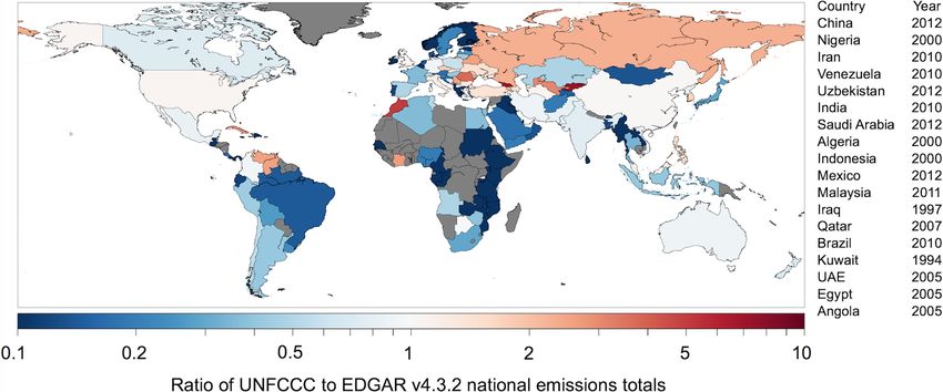
T. R. Scarpelli et al.: A global inventory of fuel exploitation methane                                                                    565

Figure 1. Methane emissions from oil, gas, and coal as resolved in our inventory. Emissions for oil and gas are separated into subsectors
representing the different life cycle stages. Each box in the figure corresponds to a separate 0.1◦ × 0.1◦ gridded product in the inventory.

gregated to the subsectors of Fig. 1. Annex I countries may               methods (IPCC, 2006) and then applying these relative sub-
choose to report emissions for a given subsector as “included             sector and process contributions to the reported emissions.
elsewhere”, which means the emissions have been included                  We multiply the IPCC Tier 1 emission factor for each subsec-
in the emissions total reported for a different subsector. The            tor to national activity data from the U.S. Energy and Infor-
most common example is when venting and flaring emissions                 mation Administration (EIA, 2018a). Oil production volume
are included within reported leakage emissions, as is the case            is used as activity data for emissions from oil exploration
for oil and gas venting and flaring in the United States. We do           and production, while volume of oil refined is used for oil
not attempt to separate these emissions here because it does              refining emissions. Oil transported by pipeline (oil produc-
not affect the spatial allocation of emissions.                           tion and imported volume) is used for oil transport leakage
   The emissions reported for oil, gas, and coal by non-                  emissions, and 50 % of oil production volume is used for oil
Annex I countries have to be disaggregated to the subsec-                 transport venting emissions (assumed to occur during truck
tors of Fig. 1. If a non-Annex I country does not report coal             and rail transport). Total gas production volume is used as
emissions separate from oil and gas, we treat it as a non-                activity data for gas production and processing, marketable
reporting country (Sect. 2.1.3). Some non-Annex I countries               gas volume (consumed gas and exported gas) is used for
choose to report oil and gas emissions by subsectors similar              gas transmission and storage, and gas consumption is used
to Annex I countries. These reported emissions are not avail-             for gas distribution. Disaggregated subsector emissions from
able in the GHG Data Interface and require inspection of re-              non-Annex I countries are then adjusted to 2016, if neces-
ports submitted by each country, including National Commu-                sary, using the EIA activity data.
nications (submitted every 4 years; COP, 2002) and Biennial                  We disaggregate Annex I venting and flaring emissions us-
Update Reports (submitted every 2 years; COP, 2011). We                   ing the relative contribution of each subsector to total venting
inspect reports for countries with estimated or reported oil              or flaring as estimated by IPCC Tier 1 methods. We cannot
and gas emissions greater than or equal to 1 Tg a−1 . These               do this for the exploration or oil refining subsectors because
countries are Algeria, Brazil, China, India, Indonesia, Iran,             IPCC methods do not separate venting and flaring emissions
Iraq, Malaysia, Nigeria, Qatar, Saudi Arabia, Uzbekistan,                 from leaks. Instead we compare the IPCC estimate for total
and Venezuela. The extent of emissions disaggregation by                  emissions from each subsector (leakage + venting + flaring)
subsector for these non-Annex I countries varies. Algeria, In-            with the reported leakage emissions. If the IPCC emissions
dia, Malaysia, Nigeria, Saudi Arabia, and Uzbekistan report               total is greater than the reported leakage emissions we as-
similarly to Annex I countries while other countries only pro-            sume that the excess emissions can be attributed to venting
vide limited disaggregation.                                              and flaring. Venting and flaring emissions from gas storage
                                                                          and gas distribution similarly cannot be separated from leaks,
2.1.2   Disaggregation by subsectors and processes                        but we assume that leaks dominate these subsectors.

We disaggregate reported emissions as needed by estimating
emissions for each subsector and process using IPCC Tier 1

www.earth-syst-sci-data.net/12/563/2020/                                                      Earth Syst. Sci. Data, 12, 563–575, 2020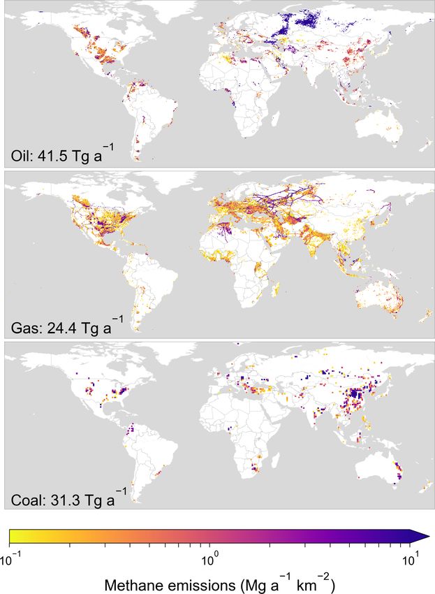
566 T. R. Scarpelli et al.: A global inventory of fuel exploitation methane
2.1.3 Non-reporting countries
For the few countries that do not report emissions from oil,
gas, and coal to the UNFCCC, we estimate emissions fol-
lowing IPCC Tier 1 methods applied to the 2016 EIA ac-
tivity data. This is notably the case for Libya and Equato-
rial Guinea, which both have total emissions greater than
0.1 Tg a−1 . We also use this method for countries that do not
report coal emissions separately from oil and gas emissions,
notably Angola, which is the only such country that has to-
tal emissions greater than 0.1 Tg a−1 . For the countries that
do not have EIA activity data, notably Uganda and Mada-
gascar, which account for most of the pipelines and wells in
such countries, we use the infrastructure data described in
Sect. 2.2 together with the average emissions per infrastruc-
ture element based on countries that do report emissions.
2.1.4 Coal emissions
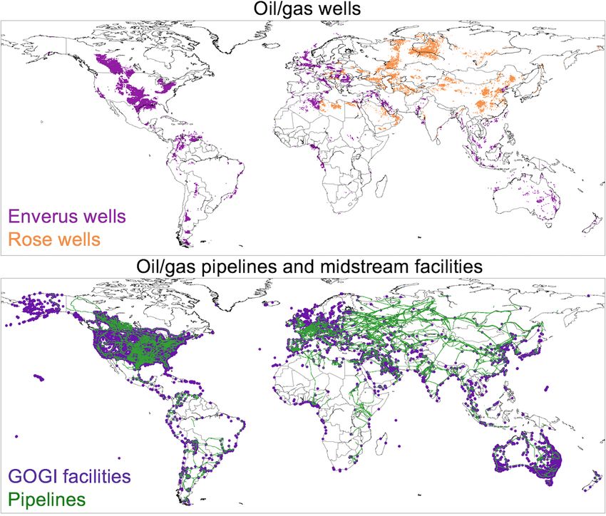
For coal, Annex I emissions for 2016 are used as reported. Figure 2. Global distributions of oil and gas wells (Enverus, 2017;
Non-Annex I emissions reported as total coal emissions are Rose, 2017), pipelines (EIA, 2018b; Petroleum Economist Ltd,
2010; Sheng et al., 2017; Sabbatino et al., 2017), and midstream
adjusted to 2016 as needed using activity data provided by
facilities (Sabbatino et al., 2017) used in our inventory. Well loca-
the EIA (2018a). For the few countries that do not report to
tions for individual countries are from the Enverus (2017) database
the UNFCCC, we use the coal emissions data embedded in where available and from the Rose (2017) database everywhere else
EDGAR v4.3.2 Fuel Exploitation with additional informa- (see text). Wells and pipelines are gridded data at 0.1◦ × 0.1◦ grid
tion from EDGAR to separate coal from oil and gas; these resolution but are shown here with 0.2◦ × 0.2◦ resolution for visi-
countries account for less than 1 % of global coal emissions. bility.
2.2 Spatially mapping emissions
2.2.1 Allocating upstream emissions to wells
Our next step is to allocate the national emissions from each
subsector of Fig. 1 spatially on a 0.1◦ × 0.1◦ grid. National Upstream emissions, including exploration and production,
emissions are allocated following the procedure described are allocated spatially to wells, as illustrated in Fig. 2. Our
below for all countries. An exception is for the contiguous principal source information on wells is Enverus (2017). It
US (Maasakkers et al., 2016) and for oil and gas in Canada provides worldwide point locations of onshore and offshore
and Mexico (Sheng et al., 2017), where we use existing in- wells, well activity status, and well content. Well activity sta-
ventories constructed for 2012 on the same 0.1◦ × 0.1◦ grid tus is used to separate active from inactive wells. Inactive
and scaled here by subsector to match the corresponding na- wells are assumed not to emit. Well content is used to sep-
tional UNFCCC reports for 2016. The two North American arate oil and gas wells, though this separation can be diffi-
inventories only provide a total oil emissions gridded prod- cult as oil wells also have production of associated gas. We
uct, and we simply scale this product to match the reported label wells as unknown content if their content is either un-
subsector totals for oil emissions. Alaska is missing from available or not clearly defined as oil or gas (this makes up
the US inventory, so we estimate emissions for Alaska us- approximately 24 % of Enverus wells outside North Amer-
ing the EPA State Inventory Tool (EPA, 2018) following the ica). We uniformly distribute emissions over the appropriate
methods outlined in the Alaska Greenhouse Gas Emission wells in each country. Within each country we determine the
Inventory (Alaska Department of Environmental Conserva- percentage of wells with unknown content and uniformly dis-
tion, 2018) and apply the procedures described below to dis- tribute this percentage of total oil and gas upstream emissions
tribute these emissions spatially. Other previously reported to those wells. We then uniformly distribute the remaining oil
gridded national emission inventories are not used here due and gas emissions to oil and gas wells, respectively.
to their limited spatial resolution and/or limited disaggre- Well data are missing from Enverus for a number of coun-
gation of emissions (Hiller et al., 2014; Höglund-Isaksson, tries. An alternative global well database with wells drilled
2012; Kurokawa et al., 2013; Wang and Bentley, 2002). We up to 2016 is available from Rose (2017) based on a com-
will use the gridded version of the UK National Atmospheric bination of open-source data and proprietary data from IHS
Emissions Inventory (NAEI; Defra and BEIS, 2019) as inde- Markit (2017) and mapped on a 0.1◦ ×0.1◦ grid (total number
pendent evaluation of our inventory in Sect. 3.3. of wells per grid cell). The Rose database does not include
information on oil versus gas content. We use this database
Earth Syst. Sci. Data, 12, 563–575, 2020 www.earth-syst-sci-data.net/12/563/2020/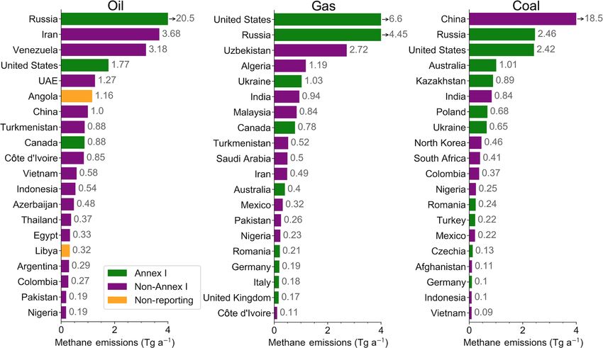
T. R. Scarpelli et al.: A global inventory of fuel exploitation methane                                                       567

for all countries that are either missing from the Enverus          that country. If the refining rate exceeds the threshold set
database or for which the Rose database has 50 % greater            by the Jamnagar Refinery in India of 1.24 million barrels
number of wells than Enverus. This includes 47 of the 134           of crude oil per day (Duddu, 2013), then oil refining emis-
countries with active well infrastructure. Of those 47 coun-        sions corresponding to the missing refineries are allocated
tries, the ones with the greatest number of wells are Russia,       to pipelines. The same is done for processing plants, stor-
United Arab Emirates (UAE), China, Libya, Saudi Arabia,             age facilities, and compressor stations. Processing plants are
Turkmenistan, Ukraine, and Azerbaijan. We distribute total          missing if production of natural gas (EIA, 2018a) distributed
upstream emissions from both oil and gas uniformly over             over processing plants exceeds 57 million cubic meters of gas
all active wells within each country. The Rose database in-         per day per facility based on the Ras Laffan processing plant
cludes offshore wells, but they are not identified by country       in Qatar (Hydrocarbons-Technology, 2017). Storage facili-
so we rely solely on Enverus for offshore wells. Between the        ties are missing if production of marketable gas (EIA, 2018a)
Enverus and Rose databases, over 99 % of global upstream            exceeds 1.9 billion m3 a−1 per facility, corresponding to the
emissions can be spatially allocated. The rest are allocated        total US capacity determined from marketable gas volume
along pipelines.                                                    and number of active storage facilities (EIA, 2015). Com-
                                                                    pressor stations are missing if the implied gas pipeline length
2.2.2   Allocating emissions to midstream infrastructure
                                                                    (CIA, 2018) between GOGI stations is more than 160 km.
                                                                       We separate the GOGI pipelines into oil and gas when
Midstream emissions from oil refining, oil transport, gas pro-      possible, though a significant number have unknown content.
cessing, gas transmission, and gas storage within a given           For each country, we determine the percentage of pipelines
country are allocated using GOGI infrastructure locations           with unknown content and distribute this percentage of to-
(Rose et al., 2018; Sabbatino et al., 2017) as shown in Fig. 2.     tal oil and gas pipeline emissions to those pipelines. The re-
Spatial information on non-well infrastructure in Alaska is         maining oil and gas emissions are allocated to oil and gas
taken from the U.S. Energy Mapping System (EIA, 2018b).             pipelines, respectively. In order to avoid allocating Russia’s
Oil refining emissions are attributed evenly to refinery loca-      significant gas transmission emissions to unknown content
tions within a given country. Oil transport emissions can oc-       pipelines, we instead use a gridded 0.1◦ × 0.1◦ map of gas
cur during pipeline, truck, or tanker transport, but we assume      pipelines based on the detailed Oil & Gas Map of Rus-
that they are mainly along pipelines and allocate them by           sia/Eurasia & Pacific Markets (Petroleum Economist Ltd,
pipeline length on a 0.1◦ × 0.1◦ grid. Gas processing, trans-       2010).
mission, and storage emissions are distributed uniformly
among the processing plant, compressor station, and stor-           2.2.3   Allocating downstream emissions
age facilities, respectively, in each country. Annex I countries
report “other” emissions for oil and gas that are distributed       Downstream gas distribution emissions are associated with
equally to wells and pipelines.                                     residential and industrial gas use. We allocate these emis-
   The GOGI database was created through a machine learn-           sions within each country on the basis of population using
ing web search of public databases for mention of oil and           the Gridded Population of the World (GPW) v4.10 30 arcsec
gas infrastructure, so it is limited to open-source informa-        map (CIESIN, 2017) for 2010. Midstream emissions are also
tion available as of 2017. It misses some infrastructure loca-      allocated to population for countries missing in the GOGI
tions (Rose et al., 2018), so the spatial allocation of emissions   database (less than 1 % of global midstream emissions).
within a country may be biased to the identified locations. To
alleviate this problem, we check each country for exceedance        2.2.4   Allocating coal emissions
of an oil or gas volume-per-facility threshold (e.g., volume of
                                                                    Coal mining and post-mining emissions from individual
gas processed per day per processing plant). These thresh-
                                                                    countries are allocated spatially to mines based on EDGAR
olds, given below, are conservative in that they are based
                                                                    v4.3.2 emission grid maps for 2012 (0.1◦ × 0.1◦ resolu-
on the world’s largest facilities or the upper limit of infras-
                                                                    tion). A specific inventory for China shows a greater num-
tructure design. If the threshold is exceeded we estimate the
                                                                    ber of mines than EDGAR v4.3.2 (Sheng et al., 2019),
percentage of facilities missing, and the corresponding per-
                                                                    but to the authors’ knowledge EDGAR is the only fine-
centage of subsector emissions is allocated to pipelines since
                                                                    resolution database of coal mine locations with global cover-
non-well infrastructure tends to lie along pipeline routes. Vi-
                                                                    age. EDGAR v4.3.2 estimates surface and underground mine
sual inspection suggests that countries with pipelines in the
                                                                    emissions separately but distributes them to mines as a com-
GOGI database are not missing any significant pipeline loca-
                                                                    bined total, so emissions from both types of mines are com-
tions which is consistent with a gap analysis for that database
                                                                    bined here. Alaskan emissions are allocated to Alaska’s sin-
(Rose et al., 2018).
                                                                    gle operational coal mine, Usibelli (EIA, 2018b).
   For oil refining in each country, we determine a refining
rate per refinery by distributing the total volume of oil re-
fined (EIA, 2018a) for 2016 over the GOGI refineries in

www.earth-syst-sci-data.net/12/563/2020/                                              Earth Syst. Sci. Data, 12, 563–575, 2020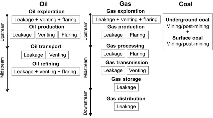
568                                                                          T. R. Scarpelli et al.: A global inventory of fuel exploitation methane

Table 1. Uncertainty ranges for IPCC emission factors and corresponding error standard deviationsa .

        Subsector                                              Annex I countries                                            Non-Annex I countries
                                              Lower (%)         Upper (%)        RSD (%)         GSD        Lower (%)         Upper (%)         RSD (%)         GSD
        Oil
              Explorationb                             100              100               50      2.11              12.5               800            100        1.79
              Production (leakage)                     100              100               50      2.11              12.5               800            100        1.79
              Production (venting)                      75               75             37.5      1.63                75                75            37.5       1.63
              Production (flaring)                      75               75             37.5      1.63                75                75            37.5       1.63
              Refining                                 100              100               50      2.11              100                100             50        2.11
              Transport (leakage)                      100              100               50      2.11                50               200            62.5       1.57
              Transport (venting)                       50               50               25      1.32                50               200            62.5       1.57
        Gas
              Explorationb                             100              100               50      2.11              12.5               800            100        1.79
              Production (leakage)                     100              100               50      2.11                40               250            72.5       1.55
              Production (flaring)                      25               25             12.5      1.14                75                75            37.5       1.63
              Processing (leakage)                     100              100               50      2.11                40               250            72.5       1.55
              Processing (flaring)                      25               25             12.5      1.14                75                75            37.5       1.63
              Transmission (leakage)                   100              100               50      1.41                40               250            72.5       1.55
              Transmission (venting)                    75               75             37.5      1.63                40               250            72.5       1.55
              Storage (leakage)                         20              500              100      1.65                20               500             100       1.65
              Distribution (leakage)                    20              500              100      1.65                20               500             100       1.65
        Coal                                            66              200             66.5      1.72                 66              200            66.5       1.72
      a The uncertainty ranges are provided by the IPCC and apply to the estimation of national emissions using emission factors specified in Tier 1 methods (IPCC,
      2006). The uncertainty range for each subsector consists of an upper bound (Upper, %) and lower bound (Lower, %) on relative emissions. We interpret each
      uncertainty range as a 95 % confidence interval and infer the corresponding relative standard deviation (RSD, %) for the assumption of a normal error pdf and
      geometric standard deviation (GSD, dimensionless) for the assumption of a lognormal pdf. The IPCC provides uncertainty ranges for “developed” and “developing”
      countries and we apply them to Annex I and non-Annex I countries, respectively. b Well drilling.

Figure 3. Methane emissions in 2016 from the top 20 emitting countries for the oil, gas, and coal sectors. Arrows next to the top bars (highest
emitting countries) indicate that emissions are not to scale.

Earth Syst. Sci. Data, 12, 563–575, 2020                                                                          www.earth-syst-sci-data.net/12/563/2020/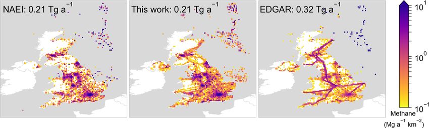
T. R. Scarpelli et al.: A global inventory of fuel exploitation methane                                                                   569

2.3   Error estimates                                             Table 2. Global methane emissions from oil, gas, and coal in 2016∗ .

                                                                              Sector/subsector                     Total (Tg a−1 )
Inverse analyses of atmospheric methane observations re-
                                                                              Oil                                               41.5
quire error estimates on the prior emission inventories as a
basis for Bayesian optimization (Jacob et al., 2016). Here we                       Exploration                                 1.4
use uncertainty ranges from IPCC (2006) to estimate error                           Production (leakage)                       17.8
standard deviations in our inventory. The IPCC reports rela-                        Production (venting)                       21.6
tive uncertainty ranges for the emission factors used in Tier                       Production (flaring)                        0.5
                                                                                    Refining                                    0.1
1 national estimates, as summarized in Table 1. Uncertain-
                                                                                    Transport (leakage)                       < 0.1
ties in national estimates are dominated by emission factors
                                                                                    Transport (venting)                       < 0.1
(typically 50 % to 100 %) as compared to the better known
activity data (5 % to 25 %; IPCC, 2006). The emission fac-                    Gas                                               24.4
tor uncertainties in Table 1 correspond to the subsectors and                       Exploration                               < 0.1
processes of our inventory (Fig. 1). We differentiate between                       Production (leakage)                        7.4
Annex I and non-Annex I countries based on IPCC uncer-                              Production (flaring)                      < 0.1
tainty ranges for “developed” and “developing” countries.                           Processing (leakage)                        2.3
   In the absence of better information, we interpret the IPCC                      Processing (flaring)                        0.1
uncertainty ranges as representing the 95 % confidence inter-                       Transmission (leakage)                      7.1
vals. The ranges are generally asymmetric, but we approxi-                          Transmission (venting)                      0.6
mate them in Table 1 in terms of either (1) a relative error                        Storage (leakage)                           1.0
                                                                                    Distribution (leakage)                      5.7
standard deviation (RSD), assuming a normal error proba-
bility density function (pdf), or (2) a geometric error stan-                 Coal                                              31.3
dard deviation (GSD), assuming a lognormal error pdf. The
                                                                              Total                                             97.2
95 % confidence interval then represents a range of 4 stan-
                                                                            ∗ From national totals reported to the UNFCCC with further
dard deviations (±2 standard deviations) in linear space for
                                                                            subsector disaggregation, year adjustment, and supplemental
the normal pdf and in log space for the lognormal pdf. For the              information as given in the text.
assumption of a normal error pdf, we take the average of the
IPCC upper and lower uncertainty limits for each subsector
and halve this value to get the RSD with an allowable maxi-       Sect. 3.3 by comparison to the UK’s independently devel-
mum RSD of 100 %. For the assumption of a lognormal error         oped gridded national inventory.
pdf, the IPCC limits are log-transformed, halved, averaged,
and transformed back to linear space to yield the GSD for
                                                                  3     Results and discussion
the lognormal error pdf. The lower limits of the IPCC uncer-
tainty ranges are capped at 90 % when determining the GSD.        3.1     Global-scale, national-scale, and grid-scale
We provide both normal and lognormal error standard devia-                emissions
tions in our inventory, as both may be useful for inverse anal-
yses. Assuming a normal error pdf has the advantage of pro-       Table 2 lists the 2016 global methane emissions from oil, gas,
viding a proper model of mean emissions, whereas assuming         and coal, broken down by the subsectors and processes re-
a lognormal error pdf has the advantage of enforcing positiv-     solved in our inventory. Total emission from fuel exploitation
ity and better allowing for anomalous emitters (Maasakkers        is 97.2 Tg a−1 , including 41.5 Tg a−1 from oil, 24.4 Tg a−1
et al., 2019).                                                    from gas, and 31.3 Tg a−1 from coal. Oil emissions are
   We assume that our large relative errors at the national       mainly from production, in part because oil fields often lack
scale can be applied directly to the 0.1◦ × 0.1◦ grid for lack    the capability to capture associated gas. Gas emissions are
of better information. An error analysis for the gridded EPA      distributed over the upstream, midstream, and downstream
inventory based on comparison to a more detailed inventory        subsectors. EDGAR v4.3.2 has a similar global total for fuel
for northeastern Texas (Barnett Shale) showed that the rela-      exploitation (107 Tg a−1 ), but the spatial distribution is very
tive error in emissions from oil systems was not significantly    different, as shown in Sect. 3.2. Top-down inverse analy-
higher on the 0.1◦ × 0.1◦ grid than the national error esti-      ses compiled by the Global Carbon Project give a range of
mate of 87 %, while the relative error for gas systems on         90–137 Tg a−1 for fuel exploitation in 2012 (Saunois et al.,
the 0.1◦ × 0.1◦ grid was twice the national estimate of 25 %      2016).
(Maasakkers et al., 2016). That work further showed that dis-        Figure 3 lists the top 20 emitting countries for oil, gas, and
placement error due to spatial misallocation of emissions is      coal in our inventory. These account for over 90 % of each
negligibly small as long as the error in emission location is     sector’s global emission. The largest emissions are from Rus-
considered isotropic. Further error evaluation is presented in    sia for oil, the US for gas, and China for coal. Oil and gas

www.earth-syst-sci-data.net/12/563/2020/                                                Earth Syst. Sci. Data, 12, 563–575, 2020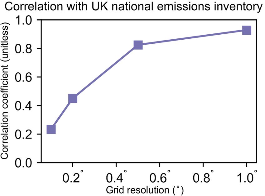
570                                                              T. R. Scarpelli et al.: A global inventory of fuel exploitation methane

                                                                          Figure 5. Total methane emissions from fuel exploitation (sum of
                                                                          oil, gas, and coal) in 2016 from this work (a) and in 2012 from
                                                                          EDGAR v4.3.2 (b; European Commission, 2017). Emissions below
                                                                          10−1 Mg a−1 km−2 are not shown.

                                                                          3.2   Comparison to the EDGAR v4.3.2 global gridded
                                                                                inventory
Figure 4. Global distribution of 2016 methane emissions from oil,
gas, and coal in our inventory. The inventory is at 0.1◦ × 0.1◦ grid
                                                                          Figure 5 compares the spatial distribution of our 2016 emis-
resolution but coal is shown here at 1◦ × 1◦ resolution for visibility.   sions from fuel exploitation (sum of the oil, gas, and coal
Emissions below 10−1 Mg a−1 km−2 are not shown.                           emissions from Fig. 4) to the corresponding 2012 emissions
                                                                          in EDGAR v4.3.2 (European Commission, 2017; Janssens-
                                                                          Maenhout et al., 2019). There are large differences between
emissions for individual countries tend to be dominated by                the inventories in terms of spatial patterns within each coun-
one of the two fuels. Notable exceptions are Russia, the US,              try, due to differences in both subsector contributions and
Iran, Canada, and Turkmenistan, which have large contribu-                spatial allocation of these contributions. Emissions along
tions from both. Annex I and non-Annex I countries report-                pipelines are generally lower in our work and emissions
ing to the UNFCCC account for 49 % and 47 % of global                     from production fields are generally higher. EDGAR v4.3.2
emissions, respectively, with the remaining 4 % of emissions              has more of a tendency to allocate midstream emissions to
contributed by countries that do not report to the UNFCCC.                pipelines rather than to specific facilities.
   Figure 4 shows the global distribution of methane emis-                   National total emissions in our inventory (based on UN-
sions separately for oil, gas, and coal. Oil emissions are                FCCC reports) are also very different from EDGAR. Fig-
mainly in production fields. Contributions from gas produc-               ure 6 compares national emissions from fuel exploitation,
tion, transmission, and distribution can all be important with            as reported to the UNFCCC versus EDGAR v4.3.2 emis-
the dominant subsector varying between countries. The high-               sions in the same year. Russia, Venezuela, and Uzbekistan
est emissions are from oil and gas production fields, gas                 report emissions that are more than a factor of 2 greater than
transmission routes, and coal mines. Most emissions along                 EDGAR v4.3.2. Iraq, Qatar, and Kuwait report emissions
gas transmission routes are from compressor stations, pro-                that are more than an order of magnitude lower than EDGAR
cessing plants, and storage facilities.                                   v4.3.2 though their last reporting years are old (1997, 2007,
                                                                          and 1994, respectively). The discrepancies between our work
                                                                          and EDGAR v4.3.2 in Russia and the Middle East lead to
                                                                          a greater emissions contribution from high latitudes and a
                                                                          lesser contribution from low latitudes in the Northern Hemi-
                                                                          sphere in our work.

Earth Syst. Sci. Data, 12, 563–575, 2020                                                   www.earth-syst-sci-data.net/12/563/2020/
T. R. Scarpelli et al.: A global inventory of fuel exploitation methane 571
Figure 6. Comparison of national methane emissions from fuel exploitation (sum of oil, gas, and coal) reported by individual countries to
the UNFCCC (2019) and estimated by the EDGAR v4.3.2 inventory (European Commission, 2017). The figure shows the ratio of UNFCCC
to EDGAR v4.3.2 national emissions, with warmer colors indicating higher UNFCCC emissions. Emissions are taken from the most recent
year reported to the UNFCCC prior to or in 2012 and compared to EDGAR for the same year. The reporting year for non-Annex I countries
with emissions greater than 1 Tg a−1 in either inventory is shown to the right. Countries in dark grey do not report fuel exploitation emissions
to the UNFCCC or have zero emissions.
The causes of differences between the UNFCCC national 3.3 Comparison to the United Kingdom national gridded
totals used in our work and EDGAR v4.3.2 are country and inventory
subsector specific because each country may choose to use a
The UK Department for Environment, Food, and Rural Af-
methodology for emissions estimation that differs from de-
fairs (Defra) and Department for Business, Energy, and In-
fault methods. Emission factors per unit of activity inferred
dustrial Strategy (BEIS) produce a gridded version of their
from the UNFCCC reports can vary by orders of magni-
annual National Atmospheric Emissions Inventory (NAEI)
tude between countries (Larsen et al., 2015). This may re-
with 0.01◦ × 0.01◦ resolution. This provides an opportunity
flect real differences in regulation of venting and flaring (es-
for evaluating our spatial allocation of emissions since the
pecially for oil production), maintenance and age of infras-
allocation in the NAEI inventory is better informed by local
tructure, and the size and number of facilities within a coun-
data, including direct reporting of emissions by large emitters
try. For example, Middle Eastern countries report low emis-
which account for 35 % of fuel exploitation emissions.
sions relative to their production volumes, and this may re-
Figure 7 compares our inventory for fuel exploitation to
flect a tendency to have a small number of high-producing
the most recent version of the NAEI in 2017 (Defra and
wells. In contrast, Russia and Uzbekistan report high emis-
BEIS, 2019) and to EDGAR v4.3.2 in 2012 (European Com-
sions relative to oil production and gas processing volumes.
mission, 2017). National totals are identical in our inven-
For Russia, differences may be due to the inclusion of ac-
tory and the NAEI, as would be expected since the NAEI
cidental releases in UNFCCC reporting, which are not con-
is used for UNFCCC reporting. The EDGAR v4.3.2 national
sidered by EDGAR v4.3.2 (Janssens-Maenhout et al., 2019).
total agrees with the 2012 NAEI (0.34 Tg a−1 ) with greater
Russia also reports large emissions from intentional venting.
coal emission compared to 2017. The differences with the
The National Report of Uzbekistan (2016) attributes their
EDGAR v4.3.2 spatial distribution are very large. Our inven-
high emissions to leaky infrastructure and recent increases
tory shows spatial distributions that are broadly consistent
in produced and transported gas volumes which may lead to
with the NAEI, with high emissions in populated areas and
operation of equipment at overcapacity. Beyond these con-
production regions. Some rural areas have zero emissions in
siderations, there may also be large errors in the emission
the NAEI but small (nonzero) emissions in our inventory be-
estimates reported by individual countries to the UNFCCC.
cause of our allocation of distribution emissions by popula-
Inverse analyses of atmospheric methane observations using
tion. These areas may in fact not have access to natural gas.
our inventory as prior estimate would provide insight into
The NAEI has fewer offshore sources than our work because
these errors.
it only accounts for the offshore wells that led to the dis-
covery of a field, rather than all wells used to exploit a field
(Tsagatakis et al., 2019).
www.earth-syst-sci-data.net/12/563/2020/ Earth Syst. Sci. Data, 12, 563–575, 2020572 T. R. Scarpelli et al.: A global inventory of fuel exploitation methane
Figure 7. Methane emissions from fuel exploitation in the United Kingdom. Our inventory (for 2016) is compared to the gridded National
Atmospheric Emissions Inventory (NAEI) for 2017 (Defra and BEIS, 2019) and EDGAR v4.3.2 for 2012 (European Commission, 2017).
Emissions below 10−1 Mg a−1 km−2 are not shown. National total emissions are given in the upper-left corner of each panel. We have
masked EDGAR offshore emissions using the other two inventories.
al., 2019). Input data and code are available upon reasonable
request.
5 Conclusions
We have constructed a global inventory of methane emis-
sions from oil, gas, and coal with 0.1◦ × 0.1◦ resolution by
spatially allocating the national emissions reported by indi-
vidual countries to the United Nations Framework Conven-
tion on Climate Change (UNFCCC). The inventory differ-
entiates oil and gas contributions from individual subsectors
along the production and supply chain and from specific pro-
Figure 8. Spatial correlation between gridded United Kingdom cesses (leakage, venting, flaring) that are then spatially allo-
emissions in our inventory and in the National Atmospheric Emis- cated using infrastructure databases. It also includes error es-
sions Inventory (NAEI; Defra and BEIS, 2019). The figure shows timates based on IPCC. Comparison with the EDGAR v4.3.2
the Pearson correlation coefficient (r) at the native 0.1◦ × 0.1◦ grid inventory shows large differences in terms of both national
resolution of our inventory and after averaging over coarser grid emissions and their spatial distribution. Comparison with the
resolutions up to 1◦ × 1◦ . gridded version of the UK National Atmospheric Emissions
Inventory (NAEI) shows overall good agreement but signifi-
cant errors on the 0.1◦ ×0.1◦ grid that are smoothed out when
Figure 8 shows the spatial correlation coefficient of emis- our inventory is averaged on a coarser grid.
sions between our inventory and the NAEI as a function of Our inventory is designed for use as prior estimate in in-
grid resolution. The correlation is low at 0.1◦ × 0.1◦ (r = verse analyses of atmospheric methane observations aiming
0.23) but increases rapidly as grid resolution is coarsened to to improve knowledge of methane emissions. Corrections to
0.2◦ × 0.2◦ (r = 0.45), 0.5◦ × 0.5◦ (r = 0.83), and 1◦ × 1◦ emission estimates revealed by the inverse analyses can be of
(r = 0.93). At fine resolution there are slight differences in direct benefit to policy by identifying biases in the national
facility locations for coal mines in particular that lead to dis- inventories reported to UNFCCC. Our inventory is for 2016
placement errors. There are also differences in the emissions but can be readily adjusted to subsequent years by updating
from individual facilities reported to the NAEI that are not the reported UNFCCC emissions and the Energy Information
resolved in our inventory. These errors are rapidly smoothed Administration’s (EIA) activity data, assuming that the spa-
out as the inventory is averaged over a coarser grid. tial distribution of emissions changes slowly. The validity of
this assumption will depend on the country and on the time
horizon for the adjustment. In North America at least, there
4 Data availability has been little change over the past decade in spatial patterns
of anthropogenic methane observed with the GOSAT satel-
The annual gridded emission fields and gridded errors for lite instrument (Sheng et al., 2018).
each subsector in Fig. 1 are available on the Harvard Data-
verse at https://doi.org/10.7910/DVN/HH4EUM (Scarpelli et
Earth Syst. Sci. Data, 12, 563–575, 2020 www.earth-syst-sci-data.net/12/563/2020/T. R. Scarpelli et al.: A global inventory of fuel exploitation methane 573
Author contributions. TRS compiled data sets and created the COP: Report of the Conference of the Parties on its seventeenth ses-
inventory. DJJ conceived of and provided guidance for the project. sion (FCCC/CP/2011/9/Add.1), Decision 2, Annex III, Durban,
JDM and JS provided guidance on North American inventories. South Africa, 28 November–11 December 2011.
MPS assisted in processing of spatial data. KR and LR processed Crippa, M., Oreggioni, G., Guizzardi, D., Muntean, M., Schaaf, E.,
and provided guidance for the infrastructure spatial data. JRW pro- LoVullo, E., Solazzo, E., Monforti-Ferrario, F., Olivier, J. G. J.,
vided guidance and feedback during inventory construction. GJM and Vignati, E.: Fossil CO2 and GHG emissions of all world
was consulted for EDGAR comparison. All authors reviewed the countries – 2019 Report, EUR 29849 EN, Publications Office
resulting inventory and assisted with paper writing. of the European Union, Luxembourg, ISBN 978-92-76-11100-9,
https://doi.org/10.2760/687800, 2019.
Defra and BEIS: National Atmospheric Emissions Inventory,
Competing interests. The authors declare that they have no con- Crown copyright 2019 under the Open Government Licence
flict of interest. (OGL), available at: http://naei.beis.gov.uk/, last access: Decem-
ber 2019.
Duddu, P.: Top 10 large oil refineries, available at: http://
Acknowledgements. This work was supported by the NASA hydrocarbons-technology.com/ (last access: June 2018), 2013.
Earth Science Division and by the NDSEG (National Defense Sci- Duren, R. M., Thorpe, A. K., Foster, K. T., Rafiq, T., Hopkins, F. M.,
ence and Engineering Graduate) Fellowship to TRS. Yadav, V., Bue, B. D., Thompson, D. R., Conley, S., Colombi, N.
K., Frankenberg, C., McCubbin, I. B., Eastwood, M. L., Falk, M.,
Herner, J. D., Croes, B. E., Green, R. O., and Miller, C. E.: Cali-
fornia’s methane super-emitters, Nature, 575, 180–184, 2019.
Financial support. This work has been supported by the ND-
EIA: The Basics of Underground Natural Gas Storage, available at:
SEG (National Defense Science and Engineering Graduate) Fellow-
http://eia.gov/naturalgas/storage/basics/ (last access: June 2018),
ship to Tia R. Scarpelli and by the NASA Earth Science Division
2015.
(NASA-Goddard Space Flight Center; grant nos. 80NSSC18K0178
EIA: International Energy Statistics, available at: http://eia.gov/
and NNX17AK81G).
beta/international/, last access: June 2018a.
EIA: U.S. Energy Mapping System, available at: https://www.eia.
gov/state/maps.php, last access: June 2018b.
Review statement. This paper was edited by Vinayak Sinha and Enverus: Enverus International, available at: http://drillinginfo.
reviewed by two anonymous referees. com/, last access: June 2017.
EPA: State Inventory and Projection Tool, avail-
able at: https://www.epa.gov/statelocalenergy/
download-state-inventory-and-projection-tool, last access:
References June 2018.
European Commission: Emission Database for Global Atmo-
Alaska Department of Environmental Conservation: Alaska spheric Research (EDGAR), 527 release version 4.2, available
Greenhouse Gas Emission Inventory 1990–2015, avail- at: http://edgar.jrc.ec.europa.eu/overview.php?v=42 (last access:
able at: https://dec.alaska.gov/air/anpms/projects-reports/ June 2018), 2011.
greenhouse-gas-inventory, last access: June 2018. European Commission: Emission Database for Global Atmospheric
Allen, D. T., Sullivan, D. W., Zavala-Araiza, D., Pacsi, A. P., Har- Research (EDGAR), release version 4.3.2, available at: http:
rison, M., Keen, K., Fraser, M. P., Daniel Hill, A., Lamb, B. K., //edgar.jrc.ec.europa.eu/overview.php?v=432&SECURE=123
Sawyer, R. F., and Seinfeld, J. H.: Methane Emissions from Pro- (last access: June 2018), 2017.
cess Equipment at Natural Gas Production Sites in the United European Commission: Emission Database for Global Atmospheric
States: Liquid Unloadings, Environ. Sci. Technol., 49, 641–648, Research (EDGAR), release version 5, available at: https://edgar.
2015. jrc.ec.europa.eu/overview.php?v=50_GHG, last access: Decem-
Brantley, H. L., Thoma, E. D., Squier, W. C., Guven, B. B., ber 2019.
and Lyon, D.: Assessment of Methane Emissions from Oil and Hiller, R. V., Bretscher, D., DelSontro, T., Diem, T., Eugster,
Gas Production Pads using Mobile Measurements, Environ. Sci. W., Henneberger, R., Hobi, S., Hodson, E., Imer, D., Kreuzer,
Technol., 48, 14508–14515, 2014. M., Künzle, T., Merbold, L., Niklaus, P. A., Rihm, B., Schel-
CIA: The World Factbook 2018, Washington, DC, available at: lenberger, A., Schroth, M. H., Schubert, C. J., Siegrist, H.,
http://cia.gov/library/publications/the-world-factbook, last ac- Stieger, J., Buchmann, N., and Brunner, D.: Anthropogenic
cess: June 2018. and natural methane fluxes in Switzerland synthesized within
CIESIN (Center for International Earth Science Information Net- a spatially explicit inventory, Biogeosciences, 11, 1941–1959,
work) Columbia University: Gridded Population of the World, https://doi.org/10.5194/bg-11-1941-2014, 2014.
Version 4 (GPWv4), Population Count Adjusted to Match 2015 Hoesly, R. M., Smith, S. J., Feng, L., Klimont, Z., Janssens-
Revision of UN WPP Country Totals, Revision 10, NASA So- Maenhout, G., Pitkanen, T., Seibert, J. J., Vu, L., Andres, R.
cioeconomic Data and Applications Center (SEDAC), Palisades, J., Bolt, R. M., Bond, T. C., Dawidowski, L., Kholod, N.,
NY, https://doi.org/10.7927/H4JQ0XZW, 2017. Kurokawa, J.-I., Li, M., Liu, L., Lu, Z., Moura, M. C. P.,
COP: Report of the Conference of the Parties on its eighth ses- O’Rourke, P. R., and Zhang, Q.: Historical (1750–2014) anthro-
sion (FCCC/CP/2002/7/Add.2), Decision 17, New Delhi, India, pogenic emissions of reactive gases and aerosols from the Com-
23 October–1 November 2002.
www.earth-syst-sci-data.net/12/563/2020/ Earth Syst. Sci. Data, 12, 563–575, 2020574 T. R. Scarpelli et al.: A global inventory of fuel exploitation methane munity Emissions Data System (CEDS), Geosci. Model Dev., 11, and Fischer, M. L.: Gridded National Inventory of U.S. Methane 369–408, https://doi.org/10.5194/gmd-11-369-2018, 2018. Emissions, Environ. Sci. Technol., 50, 13123–13133, 2016. Höglund-Isaksson, L.: Global anthropogenic methane emissions Maasakkers, J. D., Jacob, D. J., Sulprizio, M. P., Scarpelli, T. R., 2005–2030: technical mitigation potentials and costs, Atmos. Nesser, H., Sheng, J.-X., Zhang, Y., Hersher, M., Bloom, A. Chem. Phys., 12, 9079–9096, https://doi.org/10.5194/acp-12- A., Bowman, K. W., Worden, J. R., Janssens-Maenhout, G., and 9079-2012, 2012. Parker, R. J.: Global distribution of methane emissions, emis- Hydrocarbons-Technology: Dolphin Gas Project, Ras Laffan, sion trends, and OH concentrations and trends inferred from available at: http://hydrocarbons-technology.com/projects/ an inversion of GOSAT satellite data for 2010–2015, Atmos. dolphin-gas/ (last access: June 2018), 2017. Chem. Phys., 19, 7859–7881, https://doi.org/10.5194/acp-19- IHS Markit: Enerdeq Browser, available at: https://ihsmarkit.com/ 7859-2019, 2019. products/oil-gas-tools-enerdeq-browser.html (last access: July Mitchell, A. L., Tkacik, D. S., Roscioli, J. R., Herndon, S. C., Ya- 2015), 2017. covitch, T. I., Martinez, D. M., Vaughn, T. L., Williams, L. L., IPCC: Chapter 4: Fugitive Emissions, in: 2006 IPCC Guidelines Sullivan, M. R., Floerchinger, C., Omara, M., Subramanian, R., for National Greenhouse Gas Inventories, edited by: Eggleston, Zimmerle, D., Marchese, A. J., and Robinson, A. L.: Measure- H. S., Buendia, L., Miwa, K., Ngara, T., Tanabe, K., Volume ments of Methane Emissions from Natural Gas Gathering Facil- 2: Energy, The National Greenhouse Gas Inventories Program, ities and Processing Plants: Measurement Results, Enviro. Sci. Hayama, Kanagawa, Japan, 2006. Technol., 49, 3219–3227, 2015. Jacob, D. J., Turner, A. J., Maasakkers, J. D., Sheng, J., Sun, Myhre, G., Shindell, D., Bréon, F.-M., Collins, W., Fuglestvedt, K., Liu, X., Chance, K., Aben, I., McKeever, J., and Franken- J., Huang, J., Koch, D., Lamarque, J.-F., Lee, D., Mendoza, berg, C.: Satellite observations of atmospheric methane and B., Nakajima, T., Robock, A., Stephens, G., Takemura, T., and their value for quantifying methane emissions, Atmos. Chem. Zhang, H.: Anthropogenic and Natural Radiative Forcing, in: Phys., 16, 14371–14396, https://doi.org/10.5194/acp-16-14371- Climate Change 2013: The Physical Science Basis. Contribution 2016, 2016. of Working Group I to the Fifth Assessment Report of the Inter- Janssens-Maenhout, G., Crippa, M., Guizzardi, D., Muntean, M., governmental Panel on Climate Change, edited by: Stocker, T. Schaaf, E., Dentener, F., Bergamaschi, P., Pagliari, V., Olivier, J. F., Qin, D., Plattner, G.-K., Tignor, M., Allen, S. K., Boschung, G. J., Peters, J. A. H. W., van Aardenne, J. A., Monni, S., Doer- J., Nauels, A., Xia, Y., Bex, V., and Midgley, P. M., Cambridge ing, U., Petrescu, A. M. R., Solazzo, E., and Oreggioni, G. D.: University Press, Cambridge, UK and New York, NY, US, 2013. EDGAR v4.3.2 Global Atlas of the three major greenhouse gas National Report: Inventory of Anthropogenic Emissions Sources emissions for the period 1970–2012, Earth Syst. Sci. Data, 11, and Sinks of Greenhouse Gases in the Republic of Uzbekistan, 959–1002, https://doi.org/10.5194/essd-11-959-2019, 2019. 1990–2012, available at: https://unfccc.int/national_reports/ Jeong, S., Millstein, D., and Fischer, M. L.: Spatially Explicit non-annex_i_natcom/items/2979.php (last access: November Methane Emissions from Petroleum Production and the Natu- 2017), 2016. ral Gas System in California, Environ. Sci. Technol., 48, 5982– Omara, M., Sullivan, M. R., Li, X., Subramanian, R., Robinson, A. 5990, 2014. L., and Presto, A. A.: Methane Emissions from Conventional and Jeong, S., Zhao, C., Andrews, A. E., Bianco, L., Wilczak, J. Unconventional Natural Gas Production Sites in the Marcellus M., and Fischer, M. L.: Seasonal variation of CH4 emis- Shale Basin, Environ. Sci. Technol., 50, 2099–2107, 2016. sions from central California, J. Geophys. Res., 117, D11306, Peng, S., Piao, S., Bousquet, P., Ciais, P., Li, B., Lin, X., https://doi.org/10.1029/2011JD016896, 2012. Tao, S., Wang, Z., Zhang, Y., and Zhou, F.: Inventory of Kurokawa, J., Ohara, T., Morikawa, T., Hanayama, S., Janssens- anthropogenic methane emissions in mainland China from Maenhout, G., Fukui, T., Kawashima, K., and Akimoto, H.: 1980 to 2010, Atmos. Chem. Phys., 16, 14545–14562, Emissions of air pollutants and greenhouse gases over Asian re- https://doi.org/10.5194/acp-16-14545-2016, 2016. gions during 2000–2008: Regional Emission inventory in ASia Petroleum Economist Ltd: Oil & Gas Map of Russia/Eurasia & Pa- (REAS) version 2, Atmos. Chem. Phys., 13, 11019–11058, cific Markets, 1st Edn., Petroleum Economist Ltd in association https://doi.org/10.5194/acp-13-11019-2013, 2013. with VTB Capital, London, UK, 2010. Larsen, K. D., Delgado, M., and Marsters, P.: Untapped Po- Robertson, A. M., Edie, R., Snare, D., Soltis, J., Field, R. A., tential: Reducing Global Methane Emissions from Oil Burkhart, M. D., Bell, C. S., Zimmerle, D., and Murphy, S. M.: and Natural Gas Systems, Rhodium Group, available at: Variation in Methane Emission Rates from Well Pads in Four Oil https://rhg.com/research/untapped-potential-reducing-global- and Gas Basins with Contrasting Production Volumes and Com- methane-emissions-from-oil-and-natural-gas-systems/ (last positions, Environ. Sci. Technol., 51, 8832–8840, 2017. access: August 2017), 2015. Rose, K., Bauer, J., Baker, V., Bean, A., DiGiulio, J., Jones, Lyon, D. R., Zavala-Araiza, D., Alvarez, R. A., Harriss, R., Pala- K., Justman, D., Miller, R. M., Romeo, L., Sabbatino, M., cios, V., Lan, X., Talbot, R., Lavoie, T., Shepson, P., Yacovitch, and Tong, A.: Development of an Open Global Oil and T. I., Herndon, S. C., Marchese, A. J., Zimmerle, D., Robinson, Gas Infrastructure Inventory and Geodatabase, NETL-TRS-6- A. L., and Hamburg, S. P.: Constructing a Spatially Resolved 2018, NETL Technical Report Series, U.S. Department of En- Methane Emission Inventory for the Barnett Shale Region, Env- ergy, National Energy Technology Laboratory: Albany, OR, iron. Sci. Technol., 49, 8147–8157, 2015. https://doi.org/10.18141/1427573, 2018. Maasakkers, J. D., Jacob, D. J., Sulprizio, M. P., Turner, A. J., Weitz, Rose, K. K.: Signatures in the Subsurface – Big & Small Data Ap- M., Wirth, T., Hight, C., DeFigueiredo, M., Desai, M., Schmeltz, proaches for the Spatio-Temporal Analysis of Geologic Proper- R., Hockstad, L., Bloom, A. A., Bowman, K. W., Jeong, S., ties & Uncertainty Reduction, Oregon State University, available Earth Syst. Sci. Data, 12, 563–575, 2020 www.earth-syst-sci-data.net/12/563/2020/
T. R. Scarpelli et al.: A global inventory of fuel exploitation methane                                                                   575

  at: https://ir.library.oregonstate.edu/concern/graduate_thesis_or_      Sheng, J.-X., Jacob, D. J., Maasakkers, J. D., Sulprizio, M.
  dissertations/2j62s975z (last access: August 2017), PhD thesis,           P., Zavala-Araiza, D., and Hamburg, S. P.: A high-resolution
  2017.                                                                     (0.1◦ × 0.1◦ ) inventory of methane emissions from Canadian
Sabbatino, M., Romeo, L., Baker, V., Bauer, J., Barkhurst, A., Bean,        and Mexican oil and gas systems, Atmos. Environ., 158, 211–
  A., DiGiulio, J., Jones, K., Jones, T. J., Justman, D., Miller III,       215, 2017.
  R., Rose, K., and Tong., A.: Global Oil & Gas Features Database,        Sheng, J.-X., Jacob, D. J., Turner, A. J., Maasakkers, J. D., Benmer-
  https://doi.org/10.18141/1427300, 2017.                                   gui, J., Bloom, A. A., Arndt, C., Gautam, R., Zavala-Araiza, D.,
Saunois, M., Bousquet, P., Poulter, B., Peregon, A., Ciais, P.,             Boesch, H., and Parker, R. J.: 2010–2016 methane trends over
  Canadell, J. G., Dlugokencky, E. J., Etiope, G., Bastviken, D.,           Canada, the United States, and Mexico observed by the GOSAT
  Houweling, S., Janssens-Maenhout, G., Tubiello, F. N., Castaldi,          satellite: contributions from different source sectors, Atmos.
  S., Jackson, R. B., Alexe, M., Arora, V. K., Beerling, D. J., Berga-      Chem. Phys., 18, 12257–12267, https://doi.org/10.5194/acp-18-
  maschi, P., Blake, D. R., Brailsford, G., Brovkin, V., Bruhwiler,         12257-2018, 2018.
  L., Crevoisier, C., Crill, P., Covey, K., Curry, C., Frankenberg, C.,   Tsagatakis, I., Ruddy, M., Richardson, J., Otto, A., Pearson, B., and
  Gedney, N., Höglund-Isaksson, L., Ishizawa, M., Ito, A., Joos, F.,        Passant, N.: UK Emission Mapping Methodology: A report of
  Kim, H.-S., Kleinen, T., Krummel, P., Lamarque, J.-F., Langen-            the National Atmospheric Emission Inventory 2017, Ricardo En-
  felds, R., Locatelli, R., Machida, T., Maksyutov, S., McDonald,           ergy & Environment, available at: https://naei.beis.gov.uk/data/
  K. C., Marshall, J., Melton, J. R., Morino, I., Naik, V., O’Doherty,      mapping (last access: June 2018), 2019.
  S., Parmentier, F.-J. W., Patra, P. K., Peng, C., Peng, S., Peters,     UNFCCC (United Nations Framework Convention on Climate
  G. P., Pison, I., Prigent, C., Prinn, R., Ramonet, M., Riley, W.          Change), United Nations, New York, 9 May 1992.
  J., Saito, M., Santini, M., Schroeder, R., Simpson, I. J., Spahni,      UNFCCC: Greenhouse Gas Inventory Data Interface, available
  R., Steele, P., Takizawa, A., Thornton, B. F., Tian, H., Tohjima,         at: http://di.unfccc.int/detailed_data_by_party, last access: May
  Y., Viovy, N., Voulgarakis, A., van Weele, M., van der Werf, G.           2019.
  R., Weiss, R., Wiedinmyer, C., Wilton, D. J., Wiltshire, A., Wor-       Wang, Y.-P. and Bentley, S.: Development of a spatially explicit
  thy, D., Wunch, D., Xu, X., Yoshida, Y., Zhang, B., Zhang, Z.,            inventory of methane emissions from Australia and its verifica-
  and Zhu, Q.: The global methane budget 2000–2012, Earth Syst.             tion using atmospheric concentration data, Atmos. Environ., 36,
  Sci. Data, 8, 697–751, https://doi.org/10.5194/essd-8-697-2016,           4965–4975, 2002.
  2016.                                                                   Zavala-Araiza, D., Lyon, D., Alvarez, R. A., Palacios, V., Harriss,
Scarpelli, T. R., Jacob, D. J., Maasakkers, J. D., Sulprizio,               R., Lan, X., Talbot, R., and Hamburg, S. P.: Toward a Functional
  M. P., Sheng, J.-X., Rose, K., Romeo, L., Worden, J. R.,                  Definition of Methane Super-Emitters: Application to Natural
  and Janssens-Maenhout, G.: Global Inventory of Methane                    Gas Production Sites, Environ. Sci. Technol., 49, 8167–8174,
  Emissions from Fuel Exploitation, Harvard Dataverse,                      2015.
  https://doi.org/10.7910/DVN/HH4EUM, 2019.                               Zhao, C., Andrews, A. E., Bianco, L., Eluszkiewicz, J., Hirsch,
Sheng, J., Song, S., Zhang, Y., Prinn, R. G., and Janssens-                 A., MacDonald, C., Nehrkorn, T., and Fischer, M. L.:
  Maenhout, G.: Bottom-Up Estimates of Coal Mine Methane                    Atmospheric inverse estimates of methane emissions from
  Emissions in China: A Gridded Inventory, Emission Fac-                    Central California, J. Geophys. Res.-Atmos., 114, D16302,
  tors, and Trends, Environ. Sci. Tech. Let., 6, 473–478,                   https://doi.org/10.1029/2008JD011671, 2009.
  https://doi.org/10.1021/acs.estlett.9b00294, 2019.

www.earth-syst-sci-data.net/12/563/2020/                                                     Earth Syst. Sci. Data, 12, 563–575, 2020
You can also read