Business Cycles: Real Facts and a Monetary Myth (p. 3) - Finn E. Kydland Edward C. Prescott
←
→
Page content transcription
If your browser does not render page correctly, please read the page content below
Business Cycles:
Real Facts
and a Monetary Myth (p. 3)
Finn E. Kydland
Edward C. Prescott

Vector Autoregression
Evidence on Monetarism:
Another Look at
the Robustness Debate (p. 19)
Richard M. Todd
Federal Reserve Bank of Minneapolis

Quarterly Review
Vol. 14, No. 2         ISSN 0271-5287

This publication primarily presents economic research aimed at improving
policymaking by the Federal Reserve System and other governmental
authorities.

Produced in the Research Department. Edited by Preston J. Miller, Kathleen
S. Rolfe, and Inga Velde. Graphic design by Barbara Birr, Public Affairs
Department.

Address questions to the Research Department, Federal Reserve Bank,
Minneapolis, Minnesota 55480 (telephone 612-340-2341).

Articles may be reprinted if the source is credited and the Research
Department is provided with copies of reprints.

The views expressed herein are those of the authors and not
necessarily those of the Federal Reserve Bank of Minneapolis or
the Federal Reserve System.
Federal Reserve Bank of Minneapolis
   Quarterly Review Spring 1990

   Business Cycles: Real Facts and a Monetary Myth*

   Finn E. Kydland                               Edward C. Prescott
  Professor of Economics                         Adviser
  Graduate School of Industrial Administration   Research Department
  Carnegie-Mellon University                     Federal Reserve Bank of Minneapolis
                                                 and Professor of Economics
                                                 University of Minnesota

Ever since Koopmans (1947) criticized Burns and                  size that the aggregate time series under consideration
Mitchell's (1946) book on Measuring Business Cycles              are generated by some probability model, which the
as being ''measurement without theory," the reporting            economists must then estimate and test. Koopmans
of business cycle facts has been taboo in economics. In          convinced the economics profession that to do other-
his essay, Koopmans presents two basic criticisms of             wise is unscientific. On this point we strongly disagree
Burns and Mitchell's study. The first is that it provides        with Koopmans: We think he did economics a grave
no systematic discussion of the theoretical reasons for          disservice, because the reporting of facts—without
including particular variables over others in their empir-       assuming the data are generated by some probability
ical investigation. Before variables can be selected,            model—is an important scientific activity. We see no
Koopmans argues, some notion is needed of the theory             reason for economics to be an exception.
that generates the economic fluctuations. With this first           As a spectacular example of facts influencing the
criticism we completely agree: Theory is crucial in              development of economic theory, we refer to the
selecting which facts to report.                                 growth facts that came out of the empirical work of
    Koopmans' second criticism is that Burns and Mitch-          Kuznets and others. According to Solow (1970, p. 2),
ell's study lacks explicit assumptions about the proba-          these facts were instrumental in the development of his
bility distribution of the variables. That is, their study       own neoclassical growth model, which has since be-
lacks "assumptions expressing and specifying how                 come the most important organizing structure in macro-
random disturbances operate on the economy through               economics, whether the issue is one of growth or
the economic relationships between the variables"                fluctuations or public finance. Loosely paraphrased, the
(Koopmans 1947, p. 172). What Koopmans has in                    key growth facts that Solow lists (on pp. 2-3) are
mind as such relationships is clear when he concludes
                                                                      • Real output per worker (or per worker-hour) grows
an overview of Burns and Mitchell's so-called measures
                                                                        at a roughly constant rate over extended time
with this sentence: "Not a single demand or supply
schedule or other equation expressing the behavior of                   periods.
men [i.e., people] or the technical laws of production is             • The stock of real capital, crudely measured, grows
employed explicitly in the book, and the cases of                       at a roughly constant rate which exceeds the
implicit use are few and far between" (p. 163). Koop-                   growth rate of labor input.
mans repeatedly stresses this need for using a structural
system of equations as an organizing principle (pp.
169-70). Economists, he argues, should first hypothe-                 •The authors thank the National Science Foundation for financial support.

                                                                                                                                             3
• The growth rates of real output and the stock of         deviations of aggregate real output from trend. We
      capital goods tend to be similar, so the capital-to-     complete his definition by providing an explicit pro-
      output ratio shows no systematic trend.                  cedure for calculating a time series trend that success-
    • The rate of profit on capital has a horizontal trend.    fully mimics the smooth curves most business cycle
                                                               researchers would draw through plots of the data. We
These facts are neither estimates nor measures of              also follow Lucas in viewing the business cycle facts as
anything; they are obtained without first hypothesizing        the statistical properties of the comovements of devia-
that the time series are generated by a probability            tions from trend of various economic aggregates with
model belonging to some class. From this example, no           those of real output.
one can deny that the reporting of growth facts has                Lucas' definition differs importantly from that of
scientific value: Why else would Kuznets have received         Mitchell (1913, 1927), whose definition had guided
a Nobel Prize for this work? Or Solow, as well, for            students of business cycles up until World War II.
developing a parsimonious theory that rationalizes             Mitchell represents business cycles as sequences of ex-
these facts—namely, his neoclassical growth model?             pansions and contractions, particularly emphasizing
   The growth facts are not the only interesting features      turning points and phases of the cycle. We think the
of these aggregate time series. Also of interest are the       developments in economic theory that followed Mitch-
more volatile changes that occur in these and other            ell's work dictate Lucas' representation of cycles.
aggregates—that is, the cyclical behavior of the time              Equipped with our operational definition of cyclical
series. These observations are interesting because they        deviations, we present what we see as the key business
apparently conflict with basic competitive theory, in          cycle facts for the United States economy in the post-
which outcomes reflect people's ability and willingness        Korean War period (1954-1989). Some of these facts
to substitute between consumption and leisure at a             are fairly well known; others, however, are likely to
given point in time and between consumption at dif-            come as a surprise because they are counter to beliefs
ferent points in time.                                         often stated in the literature.
   The purpose of this article is to present the business          An important example of one of these commonly
cycle facts in light of established neoclassical growth        held beliefs is that the price level always has been
theory, which we use as the organizing framework for           procyclical and that, in this regard, the postwar period is
our presentation of business cycle facts. We emphasize         no exception. Even Lucas (1977, p. 9) lists procyclical
that the statistics reported here are not measures of          price levels among business cycle regularities. This
anything; rather, they are statistics that display interest-   perceived fact strongly influenced business cycle re-
ing patterns, given the established neoclassical growth        search in the 1970s. A more recent example of this
theory. In discussions of business cycle models, a             misbelief is when Bernanke (1986, p. 76) discusses a
natural question is, Do the corresponding statistics for       study by King and Plosser (1984): "Although some
the model economy display these patterns? We find              points of their analysis could be criticized (for example,
these features interesting because the patterns they           there is no tight explanation of the relation between
seem to display are inconsistent with the theory.              transaction services and the level of demand deposits,
   The study of business cycles flourished from the            and the model does not yield a strong prediction of price
1920s through the 1940s. But in the 1950s and 1960s,           procyclicality), the overall framework is not implau-
with the development of the structural system-of-              sible." Even more recently, Mankiw (1989, p. 88), in
equations approach that Koopmans advocated, busi-              discussing the same paper, points out that "while the
ness cycles ceased to be an active area of economic            story of King and Plosser can explain the procyclical
research. Now, once again, the study of business cycles,       behavior of money, it cannot explain the procyclical
in the form of recurrent fluctuations, is alive. At the        behavior of prices." We shall see that, in fact, these
leading research centers, economists are again con-            criticisms are based on what is a myth. We show that
cerned with the question of why, in market economies,          during the 35 years since the Korean War, the price
aggregate output and employment undergo repeated               level has displayed a clear countercyclical pattern.
fluctuations about trend.1                                         Other misperceptions we expose are the beliefs that
   Instrumental in bringing business cycles back into
the mainstream of economic research is the important               1
                                                                     The view of Hayek (1933, p. 33) in the 1930s and Lucas (1977, p. 7) in the
paper by Lucas (1977), "Understanding Business Cy-             1970s is that answering this question is one of the outstanding challenges to
cles." We follow Lucas in defining business cycles as the      economic research.

4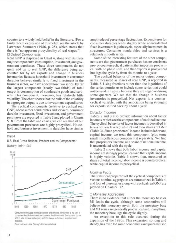
Finn E. Kydland, Edward C. Prescott
   Business Cycles

the real wage is either countercyclical or essentially            inevitably evolve from one into another: prosperity,
uncorrelated with the cycle and that the money stock,             crisis, depression, and revival. This view is expressed
whether measured by the monetary base or by Ml,                   perhaps most clearly by Mitchell ([1923] 1951, p. 46),
leads the cycle.                                                  who writes: "Then in order will come a discussion of
   The real facts documented in this paper are that               how prosperity produces conditions which lead to
major output components tend to move together over                crises, how crises run into depressions, and finally how
the cycle, with investment in consumer and producer               depressions after a time produce conditions which lead
durables having several times larger percentage devia-            to new revivals." Mitchell clearly had in mind a
tions than does spending on nondurable consumption.               theoretical framework consistent with that view. In
                                                                  defending the use of the framework of four distinct
Alternative Views of Business Cycles                              cyclical phases, Mitchell later wrote that "most current
To many, when we talk about cycles, the picture that              theories explain crises by what happens in prosperity
comes to mind is a sine wave with its regular and re-             and revivals by what happens in depression" (Mitchell
current pattern. In economics and other sciences, how-            1927, p. 472). (For an extensive overview of these
ever, the term cycle refers to a more general concept.            theories and their relationship to Mitchell's descriptive
One of the best-known examples of cycles is the sun-              work, see Haberler 1937.)
spot cycle, which varies in length from under 10 years
                                                                     We now know how to construct model economies
to nearly 20 years. The significant fact about cycles is
                                                                  whose equilibria display business cycles like those
the recurrent nature of the events.
                                                                  envisioned by Mitchell. For example, a line of research
     In 1922, at a Conference on Cycles, representatives          that gained attention in the 1980s demonstrates that
from several sciences discussed the cyclical phenomena            cyclical patterns of this form result as equilibrium
in their fields. The participants agreed on the following         behavior for economic environments with appropriate
definition (quoted in Mitchell 1927, p. 377) as being             preferences and technologies. (See, for example, Ben-
reasonable for all the sciences: "In general scientific use       habib and Nishimura 1985 and Boldrin 1989.) Burns
. . . the word (cycle) denotes a recurrence of different          and Mitchell would have been much more influential if
phases of plus and minus departures, which are often              business cycle theory had evolved in this way. Koop-
susceptible of exact measurement." Our definition of              mans (1957, pp. 215-16) makes this point in his largely
business cycles is consistent with this general definition,       unnoticed "second thought" on Burns and Mitchell's
but we refer to departures as deviations.                         work on business cycles.
Mitchell's Four Phases                                               In retrospect, it is now clear that the field of business
In 1913, Wesley C. Mitchell published a major work on             cycles has moved in a completely different direction
business cycles, in it reviewing the research that had            from the one Mitchell envisioned. Theories with deter-
preceded his own. The book presents his largely                   ministic cyclical laws of motion may a priori have had
descriptive approach, which consists of decomposing a             considerable potential for accounting for business
large number of time series into sequences of cycles and          cycles; but in fact, they have failed to do so. They have
then dividing each cycle into four distinct phases. This          failed because cyclical laws of motion do not arise as
work was continued by Mitchell (1927) and by Burns                equilibrium behavior for economies with empirically
and Mitchell (1946), who defined business cycles as               reasonable preferences and technologies—that is, for
   . . . a type of fluctuation found in the aggregate economic    economies with reasonable statements of people's
   activity of nations that organize their work mainly in         ability and willingness to substitute.
   business enterprises: a cycle consists of expansions occur-
   ring at about the same time in many economic activities,       Frisch's   Pendulum
   followed by similarly general recessions, contractions, and    As early as the 1930s, some economists were develop-
   revivals which merge into the expansion phase of the next      ing business cycle models that gave rise to difference
   cycle; this sequence of changes is recurrent but not           equations with random shocks. An important example
   periodic; in duration business cycles vary from more than      appears in a paper by Ragnar Frisch ([1933] 1965).
   one year to ten or twelve years; they are not divisible into   Frisch was careful to distinguish between impulses in
   shorter cycles of similar character with amplitudes approx-
                                                                  the form of random shocks, on the one hand, and their
   imating their own (p. 3).
                                                                  propagation over time, on the other. In contrast with
From the discussion in their books, it is clear the authors       proponents of modern business cycle theory, he empha-
view business cycles as consisting of four phases that            sized damped oscillatory behavior. The concept of

                                                                                                                            5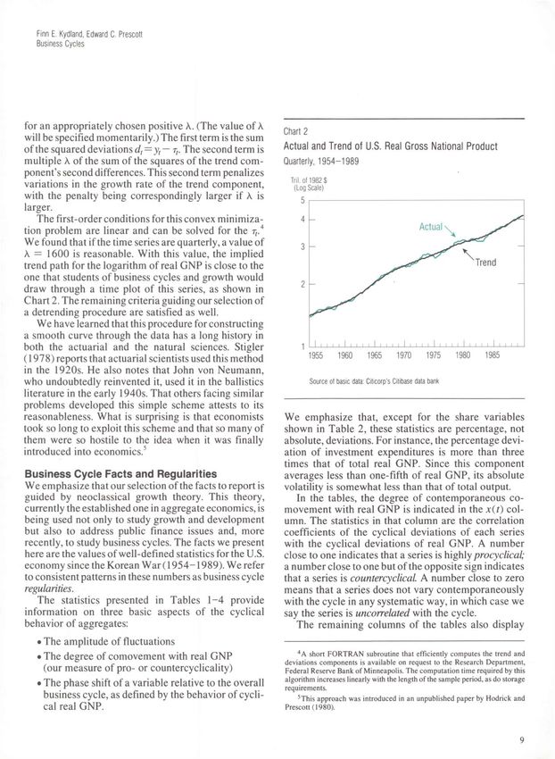
equilibrium was interpreted as a system at rest (as it is,
                                                             Chart 1
for instance, in the science of mechanics).
   The analogy of a pendulum is sometimes used to            Cycles Generated by Slutzky's Mechanism
describe this view of cycles. Shocks are needed to
provide "energy in maintaining oscillations" in damped            yt
cyclical systems. Frisch reports that he was influenced
by Knut Wicksell, to whom he attributes the following:
"If you hit a wooden rocking horse with a club, the
movement of the horse will be very different to that of
the club" (quoted in Frisch [1933] 1965, p. 178). The
use of the rocking horse and pendulum analogies under-
scores their emphasis on cycles in the form of damped
oscillations.
   The research of Frisch and Wicksell received con-
siderable attention in the 1930s, but no one built on
their work. Construction stopped primarily because the
neoclassical growth model and the necessary concep-
tual tools (particularly the Arrow-Debreu general equi-
librium theory) had not yet been developed. Since the
tools to do quantitative dynamic general equilibrium
analysis weren't available, whereas statistical time
series techniques were advancing rapidly, it's not               Chart 1 plots a time series generated in this way. The
surprising that quantitative system-of-equation mod-         time series displays patterns that Burns and Mitchell
els—especially the Keynesian income-expenditure              (1946) would characterize as business cycles.2 The
models—received virtually all the attention.                 amplitudes and duration of cycles are variable, with the
                                                             duration varying from 1 to 12 years and averaging
Slutzky's Random Shocks                                      about 3 V2 years. The time series seems to display cycles
An entirely different way of generating cycles is sug-       in Mitchell's sense of expansions containing the seed for
gested by the statistical work of Eugen Slutzky (1937).      recessions and vice versa. But, by construction, reces-
Slutzky shows that cycles resembling business fluctua-       sions do not contain the seed of subsequent expansions.
tions can be generated as the sum of random causes—          At each point in time, the expected future path is mono-
that is, by a stable, low-order, stochastic difference       tonic and converges to the zero mean, with 5 percent of
equation with large positive real roots.                     the distance being closed in each quarterly time period.
    The following exercise illustrates how Slutzky's             Another demonstration of the role that random
method can generate cycles. Let the random variable et       shocks can play appears in a paper by Adelman and
take the value 0.5 if a coin flip shows heads and —0.5 if    Adelman (1959). Using the Klein-Goldberger model,
tails. Assume that                                           they show that by adding random shocks to the model,
                                                             it produces aggregate time series that look remarka-
(1)    yt+\ = 0.95yt + et+\.                                 bly like those of the post-World War II economy of the
                                                             United States. The deterministic version of this model
By repeated substitutionals related to current and past      converges almost monotonically to a point. This exer-
shocks in the following way:                                 cise forcefully demonstrates that a stochastic process
                                                             can generate recurrent cycles while its deterministic
(2)    yt = et + 0.95et-{ + 0.95 V 2 + ' ' '                 version can converge monotonically.
              + 0 . 9 5 ' - ^ + 0.95%.                       Advancing to Lucas'   Deviations
                                                             In the 1940s and the 1950s, while macroeconometric
The yt are geometrically declining sums of past shocks.
Given an initial value y0 and a fair coin, this stochastic       2
                                                                   King and Plosser (1989) describe a well-defined, judgment-free scheme
difference equation can be used to generate a random         that successfully mimics the Burns and Mitchell procedure. The description of
path for the variable y.                                     the cycles in the time series plotted in Chart 1 is based on this procedure.

6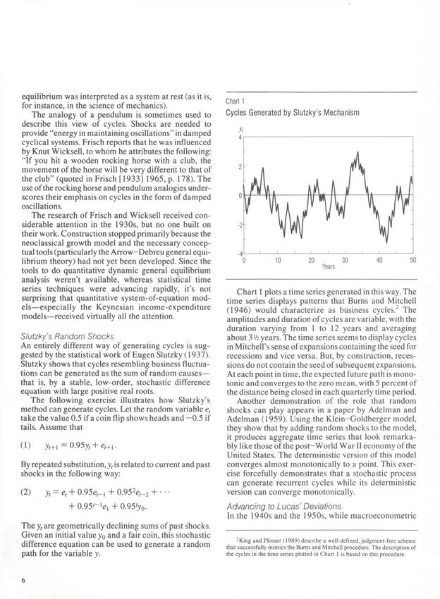
Finn E. Kydland, Edward C. Prescott
   Business Cycles

system-of-equations models were being developed,               need to distinguish among different phases of the cycle.
important theoretical advances were being made along           To Lucas, the comovements over time of the cyclical
entirely different fronts. By the early 1960s, economists'     components of economic aggregates are of primary
understanding of the way economic environments work            interest, and he gives several examples of what he views
in general equilibrium had advanced by leaps and               as the business cycle regularities. We make explicit and
bounds. The application of general equilibrium theory          operational what we mean by these terms and present a
in dynamic environments led to theoretical insights on         systematic account of the regularities. When that step is
the growth of economies; it also led to important              implemented quantitatively, some regularities emerge
measurements of the parameters of the aggregate                that, in the 1970s, would have come as a surprise—even
production function that formed the foundation for             to Lucas.
neoclassical growth theory. Thus, by the late 1960s,
there were two established theories competing for domi-        Modern Business Cycle Theory
nance in aggregate economics. One was the behavioral-          In the 1980s and now in the early 1990s, business cycles
empirical approach reflected in the Keynesian system-          (in the sense of recurrent fluctuations) increasingly
of-equations models. The other was the neoclassical            have become a focus of study in aggregate economics.
approach, which modeled environments with rational,            Such studies are generally guided by perceived business
maximizing individuals and firms. The neoclassical             cycle regularities. But if these perceptions are not in fact
approach dominated public finance, growth theory, and          the regularities, then certain lines of research are
international trade. As neoclassical theory progressed,        misguided.
an unresolvable conflict developed between the two                 For example, the myth that the price level is pro-
approaches. The impasse developed because dynamic              cyclical largely accounts for the prevalence in the
maximizing behavior is inconsistent with the assump-           1970s of studies that use equilibrium models with mon-
tion of invariant behavioral equations, an assumption          etary policy or price surprises as the main source of
that underlies the system-of-equations approach.               fluctuations. At the time, monetary disturbances ap-
   Not until the 1970s did business cycles again receive       peared to be the only plausible source of fluctuations
attention, spurred on by Lucas' (1977) article, "Un-           that could not be ruled out as being too small, so they
derstanding Business Cycles." There, Lucas viewed              were the leading candidate. The work of Friedman and
business cycle regularities as "comovements of the             Schwartz (1963) also contributed to the view that mone-
deviations from trend in different aggregative time            tary disturbances are the main source of business cycle
series." He defined the business cycle itself as the           fluctuations. Their work marshaled extensive empirical
"movements about trend in gross national product."             evidence to support the position that monetary policy is
Two types of considerations led Lucas to this definition:      an important factor in determining aggregate output,
the previously discussed findings of Slutzky and the           employment, and other key aggregates.
Adelmans, and the important advances in economic                   Since the early studies of Burns and Mitchell, the
theory, especially neoclassical growth theory. We in-          emphasis in business cycle theory has shifted from
terpret Lucas as viewing business cycle fluctuations as        essentially pure theoretical work to quantitative theo-
being of interest because they are at variance with            retical analysis. This quantitative research has had
established neoclassical growth theory.                        difficulty finding an important role for monetary
   Another important theoretical advance of the 1960s          changes as a source of fluctuations in real aggregates.
and 1970s was the development of recursive competi-            As a result, attention has shifted to the role of other
tive equilibrium theory. This theory made it possible to       factors—technological changes, tax changes, and terms-
study abstractions of the aggregate economy in which           of-trade shocks. This research has been strongly guided
optimizing economic behavior produces behavioral               by business cycle facts and regularities such as those to
relations in the form of low-order stochastic difference       be presented here.
equations. The role these advances played for Lucas'               Along with the shift in focus to investigating the
thinking is clear, as evident from one of his later articles   sources and nature of business cycles, aggregate analy-
discussing methods and problems in business cycle              sis underwent a methodological revolution. Previously,
theory (see Lucas 1980).                                       empirical knowledge had been organized in the form of
   In contrast with Mitchell's view of business cycles,        equations, as was also the case for the early rational
Lucas does not think in terms of sequences of cycles as        expectations models. Muth (1960), in his pioneering
inevitable waves in economic activity, nor does he see a       work on rational expectations, did not break with this

                                                                                                                         7
system-of-equations tradition. For that reason, his          technological change in the 1950s and 1960s was
econometric program did not come to dominate. In-            significantly above the U.S. historical average rate over
stead, the program which has prevailed is the one that       the past 100 years. In the 1970s, the rate was signifi-
organizes empirical knowledge around preferences,            cantly below average. In the 1980s, the rate was near
technology, information structure, and policy rules or       the historical average. Because the underlying rate of
arrangements. Sargent (1981) has led the development         technological change has not been constant in the
of tools for inferring values of parameters character-       period we examine (1954-1989), detrending using a
izing these elements, given the behavior of the ag-          linear function of time is inappropriate. The scheme
gregate time series. As a result, aggregate economics is     used must let the average rate of technological change
no longer a separate and entirely different field from the   vary over time, but not too rapidly.
rest of economics; it now uses the same tools and                Any definition of the trend and cycle components,
empirical knowledge as other branches of economics,          and for that matter the seasonal component, is neces-
such as finance, growth theory, public finance, and          sarily statistical. A decomposition is a representation of
international economics. With this development, mea-         the data. A representation is useful if, in light of theory,
surements and quantitative findings in those other fields    it reveals some interesting patterns in the data. We think
can be used to restrict models of business cycles and        our representation is successful in this regard. Our selec-
make our knowledge about the quantitative importance         tion of a trend definition was guided by the following
of cyclical disturbances more precise.                       criteria:
                                                                   • The trend component for real GNP should be ap-
Business Cycle Deviations Redefined
                                                                     proximately the curve that students of business
Because economic activity in industrial market econo-
                                                                     cycles and growth would draw through a time plot
mies is characterized by sustained growth, Lucas
                                                                     of this time series.
defines business cycles as deviations of real gross
national product (GNP) from trend rather than from                 • The trend of a given time series should be a linear
some constant or average value. But Lucas does not                   transformation of that time series, and this transfor-
define trend, so his definition of business cycle devia-             mation should be the same for all series.3
tions is incomplete. What guides our, and we think his,            • Lengthening the sample period should not signifi-
concept of trend is steady state growth theory. With this            cantly alter the value of the deviations at a given
theory there is exogenous labor-augmenting technolog-                date, except possibly near the end of the original
ical change that occurs at a constant rate; that is, the             sample.
effectiveness of labor grows at some constant rate.                • The scheme should be well defined, judgment free,
Steady state growth is characterized by per capita                   and cheaply reproducible.
output, consumption, investment, capital stock, and the
real wage all growing at the same rate as does tech-             These criteria led us to the following scheme. Let yt,
nology. The part of productive time allocated to market      for t = 1 , 2 , . . . ,T, denote a time series. We deal with
activity and the real return on capital remain constant.     logarithms of a variable, unless the variable is a share,
   If the rate of technological change were constant,        because the percentage deviations are what display the
then the trend of the logarithm of real GNP would be a       interesting patterns. Moreover, when an exponentially
linear function of time. But the rate of technological       growing time series is so transformed, it becomes linear
change varies both over time and across countries.           in time. Our trend component, denoted rr, for t = 1,2,...,
(Why it varies is the central problem in economic            T} is the one that minimizes
development or maybe in all of economics.) The rate of
change clearly is related to the arrangements and
                                                             (3)        5£=,o>,-T,)2
institutions that a society uses and, more important, to
the arrangements and institutions that people expect                            + X2[=2'[(r1+1-r,)-(r-r(_1)]2
will be used in the future. Even in a relatively stable
society like the United States since the Second World             3
                                                                    The reason for linearity is that the first two moments of the transformed
War, there have been significant changes in institutions.    data are functions of the first two moments, and not the higher moments, of the
And when a society's institutions change, there are          original data. The principal rationale for the same transformation being applied
                                                             to all time series is that it makes little sense to carry out the analogue of growth
changes in the productivity growth of that society's         accounting with the inputs to the production function subject to one transfor-
labor and capital. In the United States, the rate of         mation and the outputs subject to another.

8
Finn E. Kydland, Edward C. Prescott
   Business Cycles

for an appropriately chosen positive A. (The value of A
                                                              Chart 2
will be specified momentarily.) The first term is the sum
of the squared deviations dt — yt— rt. The second term is     Actual and Trend of U.S. Real Gross National Product
multiple k of the sum of the squares of the trend com-        Quarterly, 1 9 5 4 - 1 9 8 9
ponent's second differences. This second term penalizes
                                                                Tril. of 1982 $
variations in the growth rate of the trend component,
with the penalty being correspondingly larger if A is
larger.
    The first-order conditions for this convex minimiza-
tion problem are linear and can be solved for the r,.4
We found that if the time series are quarterly, a value of
A = 1600 is reasonable. With this value, the implied
trend path for the logarithm of real GNP is close to the
one that students of business cycles and growth would
draw through a time plot of this series, as shown in
Chart 2. The remaining criteria guiding our selection of
a detrending procedure are satisfied as well.
    We have learned that this procedure for constructing
a smooth curve through the data has a long history in
both the actuarial and the natural sciences. Stigler
(1978) reports that actuarial scientists used this method
in the 1920s. He also notes that John von Neumann,
who undoubtedly reinvented it, used it in the ballistics                Source of basic data: Citicorp's Citibase data bank
literature in the early 1940s. That others facing similar
problems developed this simple scheme attests to its
reasonableness. What is surprising is that economists         We emphasize that, except for the share variables
took so long to exploit this scheme and that so many of       shown in Table 2, these statistics are percentage, not
them were so hostile to the idea when it was finally          absolute, deviations. For instance, the percentage devi-
introduced into economics.5                                   ation of investment expenditures is more than three
                                                              times that of total real GNP. Since this component
Business Cycle Facts and Regularities                         averages less than one-fifth of real GNP, its absolute
We emphasize that our selection of the facts to report is     volatility is somewhat less than that of total output.
guided by neoclassical growth theory. This theory,               In the tables, the degree of contemporaneous co-
currently the established one in aggregate economics, is      movement with real GNP is indicated in the x(t) col-
being used not only to study growth and development           umn. The statistics in that column are the correlation
but also to address public finance issues and, more           coefficients of the cyclical deviations of each series
recently, to study business cycles. The facts we present      with the cyclical deviations of real GNP. A number
here are the values of well-defined statistics for the U.S.   close to one indicates that a series is highly procyclical;
economy since the Korean War (1954-1989). We refer            a number close to one but of the opposite sign indicates
to consistent patterns in these numbers as business cycle     that a series is countercyclical. A number close to zero
regularities.                                                 means that a series does not vary contemporaneously
   The statistics presented in Tables 1-4 provide             with the cycle in any systematic way, in which case we
information on three basic aspects of the cyclical            say the series is uncorrected with the cycle.
behavior of aggregates:                                          The remaining columns of the tables also display
   • The amplitude of fluctuations
                                                                  4
   • The degree of comovement with real GNP                         A short FORTRAN subroutine that efficiently computes the trend and
                                                              deviations components is available on request to the Research Department,
     (our measure of pro- or countercyclicality)              Federal Reserve Bank of Minneapolis. The computation time required by this
                                                              algorithm increases linearly with the length of the sample period, as do storage
   • The phase shift of a variable relative to the overall    requirements.
     business cycle, as defined by the behavior of cycli-         5
                                                                    This approach was introduced in an unpublished paper by Hodrick and
     cal real GNP.                                            Prescott (1980).

                                                                                                                                            9
correlation coefficients, except the series have been                                        facts to examine and how to organize them. The
shifted forward or backward, relative to real GNP, by                                        aggregate economy can be divided broadly into three
from one to five quarters. To some extent these                                              sectors: businesses, households, and government. In
numbers indicate the degree of comovement with GNP.                                          the business sector, the model emphasizes production
Their main purpose, however, is to indicate whether,                                         inputs as well as output components. Households allo-
typically, there is a phase shift in the movement of a                                       cate income earned in the business sector to consump-
time series relative to real GNP. For example, if for                                        tion and saving. In the aggregate, there is an accounting
some series the numbers in the middle of each table are                                      relation between household saving and business invest-
positive but largest in column x(t~i), where i > 0, then                                     ment. Households allocate a fraction of their discre-
the numbers indicate that the series is procyclical but                                      tionary time to income-earning activities in the business
tends to peak about i quarters before real GNP. In this                                      sector. The remaining fraction goes to nonmarket
case we say the series leads the cycle. Correspondingly,                                     activities, usually referred to as leisure but sometimes
a series that lags the cycle byj > 0 quarters would have                                     (perhaps more appropriately) as input to household
the largest correlation coefficient in the column headed                                     production. This time-allocation decision has received
by x(t+j). For example, productivity is a series that                                        little attention in growth theory, but it is crucial to
leads the cycle, whereas the stock of inventories is one                                     business cycle theory. The government sector, which is
that lags the cycle.                                                                         at the heart of public finance theory, also could play a
   We let the neoclassical growth model dictate which                                        significant role for business cycles.

Table 1
Cyclical Behavior of U.S. Production Inputs
Deviations From Trend of Input Variables
Quarterly, 1954-1989

                                                                                                      Cross Correlation of Real GNP With
                                                    vuidumy
Variable x                                        (% Std. Dev.)   x(t- 5)   x(t-A)   x(t- 3)    x(t- 2)   x(M)       x(t)    x(/+1)    x(t+ 2)    x(t+3)   x(t+4)   x(t+5)

Real Gross National Product                            1.71       -0.03       0.15    0.38       0.63       0.85      1.00     0.85        0.63    0.38      0.15   -0.03

Labor Input
     Hours (Household Survey)                          1.47       -0.10       0.05    0.23       0.44       0.69      0.86     0.86        0.75     0.59     0.38     0.18
        Employment                                     1.06       -0.18     -0.04     0.14       0.36       0.61      0.82     0.89        0.82     0.67     0.47     0.25
          Hours per Worker                             0.54        0.08       0.21    0.35       0.49       0.66      0.71     0.59        0.43    0.29      0.11   -0.02
     Hours (Establishment Survey)                      1.65       -0.23     -0.07     0.14       0.39       0.66      0.88     0.92        0.81     0.64     0.42     0.21
     GNP/Hours (Household Survey)                      0.88        0.11       0.21    0.34       0.48       0.50      0.51     0.21    -0.02      -0.25    -0.34    -0.36
     GNP/Hours (Establishment Survey)                  0.83        0.40       0.46    0.49       0.53       0.43      0.31   -0.07     -0.31      -0.49    -0.52    -0.50
     Average Hourly Real Compensation                  0.91        0.30       0.37    0.40       0.42       0.40      0.35     0.26        0.17     0.05   -0.08    -0.20
         (Business Sector)

Capital Input
     Nonresidental Capital Stock*                      0.62       -0.58     -0.61    -0.51     -0.48      -0.31    -0.08       0.16        0.39     0.56     0.66     0.70
          Structures                                   0.37       -0.45     -0.51    -0.55     -0.53      -0.44    -0.29     -0.10         0.09     0.25     0.38     0.45
          Producers' Durable Equipment                 0.99       -0.57     -0.58    -0.53     -0.41      -0.22       0.02     0.26        0.47     0.62     0.70     0.71

 Inventory Stock (Nonfarm)                             1.65       -0.37     -0.33    -0.23     -0.05        0.19      0.50     0.72        0.83     0.81     0.71     0.53

"Based on quarterly data, 1954:1-1984:2.
 Source of basic data: Citicorp's Citibase data bank

10
Finn E. Kydland, Edward C. Prescott
Business Cycles
The standard version of the neoclassical growth gates and nominal prices.
model abstracts from money and therefore provides
little guidance about which of the nominal variables to
examine. Given the prominence that monetary shocks Real Facts
have held for many years as the main candidate for the • Production Inputs
impulse to business cycles, it seems appropriate that we We first examine real (nonmonetary) series related to
also examine the cyclical behavior of monetary aggre- the inputs in aggregate production. The cyclical facts
Table 2
Cyclical Behavior of U.S. Output and Income Components
Deviations From Trend of Product and Income Variables
Quarterly, 1954-1989
Cross Correlation of Real GNP With
Volatility
Variable/ (% Std. Dev.) x(t- 5) x(M) x(t-3) x(t- 2) x(M) x(t) x(t+1) x(t+2) x(t+3) x(/+4) x(t+5)
Real Gross National Product 1.71 -0.03 0.15 0.38 0.63 0.85 1.00 0.85 0.63 0.38 0.15 -0.03
Consumption Expenditures 1.25 0.25 0.41 0.56 0.71 0.81 0.82 0.66 0.45 0.21 -0.02 -0.21
Nondurables & Services 0.84 0.20 0.38 0.53 0.67 0.77 0.76 0.63 0.46 0.27 0.06 -0.12
Nondurables 1.23 0.29 0.42 0.52 0.62 0.69 0.69 0.57 0.38 0.16 -0.05 -0.22
Services 0.63 0.03 0.25 0.46 0.63 0.73 0.71 0.60 0.49 0.39 0.23 0.07
Durables 4.99 0.25 0.38 0.50 0.64 0.74 0.77 0.60 0.37 0.10 -0.14 -0.32
Investment Expenditures 8.30 0.04 0.19 0.39 0.60 0.79 0.91 0.75 0.50 0.21 -0.05 -0.26
Fixed Investment 5.38 0.09 0.25 0.44 0.64 0.83 0.90 0.81 0.60 0.35 0.08 -0.14
Nonresidential 5.18 -0.26 -0.13 0.05 0.31 0.57 0.80 0.88 0.83 0.68 0.46 0.23
Structures 4.75 -0.40 -0.31 -0.17 0.03 0.29 0.52 0.65 0.69 0.63 0.50 0.34
Equipment 6.21 -0.18 -0.04 0.14 0.39 0.65 0.85 0.90 0.81 0.62 0.38 0.15
Residential 10.89 0.42 0.56 0.66 0.73 0.73 0.62 0.37 0.10 -0.15 -0.34 -0.45
Government Purchases 2.07 0.00 -0.03 -0.03 -0.01 -0.01 0.05 0.09 0.12 0.17 0.27 0.34
Federal 3.68 0.00 -0.05 -0.08 -0.09 -0.09 -0.02 0.03 0.06 0.10 0.19 0.24
State & Local 1.19 0.06 0.10 0.17 0.25 0.26 0.25 0.20 0.16 0.19 0.27 0.36
Exports 5.53 -0.50 -0.46 -0.34 -0.14 0.11 0.34 0.48 0.53 0.53 0.53 0.45
Imports 4.92 0.11 0.18 0.30 0.45 0.61 0.71 0.71 0.51 0.28 0.03 -0.19
Real Net National Income
Labor Income* 1.58 -0.18 -0.02 0.18 0.42 0.68 0.88 0.90 0.80 0.62 0.40 0.19
Capital Income** 2.93 0.10 0.24 0.44 0.63 0.79 0.84 0.60 0.30 0.02 -0.19 -0.29
Proprietors' Income & Misc.f 2.70 0.11 0.24 0.38 0.55 0.62 0.68 0.46 0.29 0.11 0.02 -0.10
* Employee compensation is deflated by the implicit GNP price deflator.
**This variable includes corporate profits with inventory valuation and capital consumption adjustments, plus rental income of persons with capital consumption adjustment,
plus net interest, plus capital consumption allowances with capital consumption adjustment, all deflated by the implicit GNP price deflator.
fProprietors' income with inventory valuation and capital consumption adjustments, plus indirect business tax and nontax liability, plus business transfer payments, plus
current surplus of government enterprises, less subsidies, plus statistical discrepancy.
Source of basic data: Citicorp's Citibase data bank
11are summarized in Table 1. Since it is not unreasonable The hours-worked series from the household survey
to think of the inventory stock as providing productive can be decomposed into employment fluctuations on
services, we include this series with the labor and the one hand and variations in hours per worker on the
capital inputs. other. Employment lags the cycle, while hours per
The two most common measures of the labor input worker is nearly contemporaneous with it, with only a
are aggregate hours-worked according to the house- slight lead. Much more of the volatility in total hours
hold survey and, alternatively, the payroll or establish- worked is caused by employment volatility than by
ment survey. We see in Table 1 that total hours with changes in hours per worker. If these two subseries were
either measure is strongly procyclical and has cyclical perfectly correlated, their standard deviations would
variation which, in percentage terms, is almost as large add up to the standard deviation of total hours.
as that of real GNP. (For a visual representation of this Although not perfectly correlated, their correlation is
behavior, see Chart 3.) The capital stock, in contrast, quite high, at 0.86. Therefore, employment accounts
varies smoothly over the cycle and is essentially for roughly two-thirds of the standard deviation in
uncorrelated with contemporaneous real GNP. The total hours while hours per worker accounts for about
correlation is large, however, if the capital stock is one-third.
shifted back by about a year. In other words, business As a measure of the aggregate labor input, aggregate
capital lags the cycle by at least a year. The inventory hours has a problem: it does not account for differences
stock also lags the cycle, but only by about half a year. across workers in their relative contributions to aggre-
In percentage terms, the inventory stock is nearly as gate output. That is, the hours of a brain surgeon are
volatile as quarterly real GNP. given the same weight as those of an orderly. This
Table 3
Cyclical Behavior of U.S. Output and Income Component Shares
Deviations From Trend of Product and Income Variables
Quarterly, 1954-1989
Mean Cross Correlation of Real GNP With
% of Volatility
Variablex GNP (% std. Dev.) x(/-5) x{t-4) x{t-3) x(t-2) x(M) x(t) x(M) x{t+2) x(t+3) x(t+4) x(t+5)
Gross National Product
Consumption Expenditures 63.55 0.58 0.29 0.15 -0.06 -0.32 -0.56 -0.78 -0.68 -0.52 -0.33 -0.17 -0.03
Nondurables & Services 54.79 0.70 0.06 -0.08 -0.27 -0.51 -0.72 -0.89 -0.73 -0.50 -0.23 0.01 0.18
Durables 8.76 0.33 0.36 0.43 0.48 0.54 0.56 0.53 0.36 0.15 -0.10 -0.31 -0.44
Investment Expenditures 15.85 1.07 0.03 0.18 0.36 0.56 0.75 0.87 0.71 0.47 0.18 -0.09 -0.30
Fixed Investment 15.16 0.56 0.11 0.25 0.40 0.57 0.74 0.81 0.77 0.61 0.40 0.14 -0.08
Change in Business Inventories 0.69 0.69 0.04 0.07 0.24 0.40 0.56 0.69 0.48 0.22 -0.05 -0.25 -0.40
Government Purchases 20.13 0.57 0.04 -0.09 -0.25 -0.40 -0.55 -0.61 -0.52 -0.36 -0.15 0.09 0.28
Net Exports 0.47 0.45 -0.51 -0.51 -0.48 -0.43 -0.37 -0.28 -0.17 0.00 0.17 0.30 0.38
: National Income*
Labor Income 58.57 0.47 -0.29 -0.36 -0.45 -0.52 -0.47 -0.39 -0.03 0.23 0.42 0.48 0.46
Capital Income 24.38 0.42 0.19 0.25 0.36 0.43 0.48 0.43 0.17 -0.13 -0.35 -0.48 -0.46
Proprietors' Income & Misc. 17.04 0.34 0.18 0.19 0.17 0.17 0.06 0.00 -0.16 -0.19 -0.20 -0.11 -0.11
*For explanations of the national income components, see notes to Table 2.
Source of basic data: Citicorp's Citibase data bank
12Finn E. Kydland, Edward C. Prescott
Business Cycles
disparity would not be problematic if the cyclical
Chart 3
volatility of highly skilled workers resembled that of the
Deviations From Trend of U.S. Real Gross National Product workers who are less skilled. But it doesn't. The hours of
and Hours Worked* the less-skilled group are much more variable, as
Quarterly, 1954-1989 established in one of our recent studies (Kydland and
Prescott 1989). Using data for nearly 5,000 people
from all major demographic groups over the period
1969-82, we found that, cyclically, aggregate hours is
a poor measure of the labor input. When people were
weighted by their relative human capital, the labor
input for this sample and period varied only about
two-thirds as much as did aggregate hours. We there-
fore recommend that the cyclical behavior of labor
productivity (as reported by GNP/hours in Table 1) be
interpreted with caution.
Since the human-capital-weighted cyclical measure
of labor input fluctuates less than does aggregate hours,
the implicit real wage (the ratio of total real labor
compensation to labor input) is even more procyclical
than average hourly real compensation. (For the latter
*The estimate of hours worked uses the establishment survey.
series, see Table 1.) This finding that the real wage
Source of basic data: Citicorp's Citibase data bank
behaves in a reasonably strong procyclical manner is
Table 4
Cyclical Behavior of U.S. Monetary Aggregates and the Price Level
Deviations From Trend of Money Stock, Velocity, and Price Level
Quarterly, 1954-1989
Cross Correlation of Real GNP With
Volatility
Variable x (% Std. Dev.) x(t- 5) x(t-A) x(t- 3) x(t- 2) x(M) x(t) x(M) x(t+2) x(/+3) x(/+4) x(/+5)
Nominal Money Stock*
Monetary Base 0.88 -0.12 0.02 0.14 0.25 0.36 0.41 0.40 0.37 0.32 0.28 0.26
M1 1.68 0.01 0.12 0.23 0.33 0.35 0.31 0.22 0.15 0.09 0.07 0.07
M2 1.51 0.48 0.60 0.67 0.68 0.61 0.46 0.26 0.05 -0.15 -0.33 -0.46
M2-M1 1.91 0.53 0.63 0.67 0.65 0.56 0.40 0.20 -0.01 -0.21 -0.39 -0.53
ocity*
Monetary Base 1.33 -0.26 -0.15 0.00 0.22 0.40 0.59 0.50 0.37 0.22 0.08 -0.08
M1 2.02 -0.24 -0.19 -0.12 -0.01 0.14 0.31 0.32 0.27 0.20 0.10 0.00
M2 1.84 -0.63 -0.59 -0.48 -0.29 -0.05 0.24 0.34 0.40 0.43 0.44 0.43
:e Level
Implicit GNP Deflator 0.89 -0.50 -0.61 -0.68 -0.69 -0.64 -0.55 -0.43 -0.31 -0.17 -0.04 0.09
Consumer Price Index 1.41 -0.52 -0.63 -0.70 -0.72 -0.68 -0.57 -0.41 -0.24 -0.05 0.14 0.30
* Based on quarterly data, 1959:1-1989:4.
Source of basic data: Citicorp's Citibase data bank
13counter to a widely held belief in the literature. [For a amplitudes of percentage fluctuations. Expenditures for
fairly recent expression of this belief, see the article by consumer durables leads slightly while nonresidential
Lawrence Summers (1986, p. 25), which states that fixed investment lags the cycle, especially investment in
there is "no apparent procyclicality of real wages."] structures. Consumer nondurables and services is a
• Output Components relatively smooth series.
Real GNP is displayed in Chart 4, along with its three Some of the interesting features of the other compo-
major components: consumption, investment, and gov- nents are that government purchases has no consistent
ernment purchases. These three components do not pro- or countercyclical pattern, that imports is procycli-
quite add up to real GNP, the difference being ac- cal with no phase shift, and that exports is procyclical
counted for by net exports and change in business but lags the cycle by from six months to a year.
inventories. Because household investment in consumer The cyclical behavior of the major output compo-
durables behaves similarly to fixed investment in the nents, measured as shares of real GNP, is reported in
business sector, we have added those two series. By far Table 3. Using fractions rather than the logarithms of
the largest component (nearly two-thirds) of total the series permits us to include some series that could
output is consumption of nondurable goods and serv- not be used in Table 2 because they are negative during
ices. This component, moreover, has relatively little some quarters. We see that the change in business
volatility. The chart shows that the bulk of the volatility inventories is procyclical. Net exports is a counter-
in aggregate output is due to investment expenditures. cyclical variable, with the association being strongest
The cyclical components (relative to cyclical real for exports shifted back by about a year.
GNP) of consumer nondurables and services, consumer
durable investment, fixed investment, and government • Factor Incomes
purchases are reported in Table 2 and plotted in Charts Tables 2 and 3 also provide information about factor
5-8. From the table and charts, we can see that all but incomes, which are the components of national income.
government purchases are highly procyclical. House- The cyclical behavior of factor incomes is described in
hold and business investment in durables have similar terms of their levels (Table 2) and their shares of GNP
(Table 3). Since proprietors' income includes labor and
Chart 4
capital income, we treat this component (plus some
small miscellaneous components) separately. We find
U.S. Real Gross National Product and Its Components* that proprietors' income, as a share of national income,
Quarterly, 1954-1989 is uncorrected with the cycle.
Table 2 shows that both labor income and capital
Tril. of
income are strongly procyclical and that capital income
is highly volatile. Table 3 shows that, measured as
shares of total income, labor income is countercyclical
while capital income is procyclical.
Nominal Facts
The statistical properties of the cyclical components of
various nominal aggregates are summarized in Table 4,
and four of these series along with cyclical real GNP are
plotted on Charts 9-12.
• Monetary Aggregates
There is no evidence that either the monetary base or
Ml leads the cycle, although some economists still
believe this monetary myth. Both the monetary base
and M1 series are generally procyclical and, if anything,
"Consumption includes nondurable goods and services. Investment is the sum of the monetary base lags the cycle slightly.
consumer durable investment and business fixed investment. Components do not
add to total because net exports and the change in business inventories are
An exception to this rule occurred during the
excluded. expansion of the 1980s. This expansion, so long and
Source of basic data: Citicorp's Citibase data bank steady, has even led some economists and journalists to
14Finn E. Kydland, Edward C. Prescott
Business Cycles
Charts 5 - 8
Deviations From Trend of U.S. Real Gross National Product
and Its Components
Quarterly, 1 9 5 4 - 1 9 8 9
Chart 5 Consumption of Nondurable Goods & Services Chart 6 Consumer Durable Investment
%
Chart 7 Business Fixed Investment Chart 8 Government Purchases
% %
Source of basic data: Citicorp's Citibase data bank
15Charts 9 - 1 2
Deviations From Trend of U.S. Real Gross National Product
and Selected Nominal Aggregates
Quarterly, 1959-1989*
Tor the price level, 1954-1989.
Source of basic data: Citicorp's Citibase data bank
16Finn E. Kydland, Edward C. Prescott
Business Cycles
speculate that the business cycle is dead (Zarnowitz moves countercyclical^.
1989 and The Economist 1989). During the expansion, The fact that the transaction component of real cash
Ml was uncommonly volatile, and M2, the more com- balances (Ml) moves contemporaneously with the
prehensive measure of the money stock, showed some cycle while the much larger nontransaction component
evidence that it leads the cycle by a couple quarters. (M2) leads the cycle suggests that credit arrangements
The difference in the behavior of Ml and M2 could play a significant role in future business cycle
suggests that the difference of these aggregates (M2 theory. Introducing money and credit into growth
minus M1) should be considered. This component main- theory in a way that accounts for the cyclical behavior
ly consists of interest-bearing time deposits, including of monetary as well as real aggregates is an important
certificates of deposit under $100,000. It is approxi- open problem in economics.
mately one-half of annual GNP, whereas Ml is about
one-sixth. The difference of M2 - M1 leads the cycle by
even more than M2, with the lead being about three
quarters.
From Table 4 it is also apparent that money veloc-
ities are procyclical and quite volatile.
• Price Level
Earlier in this paper, we documented the view that the
price level is always procyclical. This myth originated
from the fact that, during the period between the world
wars, the price level was procyclical. But because of the
Koopmans taboo against reporting business cycle facts,
no one bothered to ascertain the cyclical behavior of the
price level since World War II. Instead, economists just
carried on, trying to develop business cycle theories in
which the price level plays a central role and behaves
procyclically. The fact is, however, that whether mea-
sured by the implicit GNP deflator or by the consumer
price index, the U.S. price level clearly has been
countercyclical in the post-Korean War period.
Concluding Remarks
Let us reemphasize that, unlike Burns and Mitchell, we
are not claiming to measure business cycles. We also
think it inadvisable to start our economics from some
statistical definition of trend and deviation from trend,
with growth theory being concerned with trend and
business cycle theory with deviations. Growth theory
deals with both trend and deviations.
The statistics we report are of interest, given neo-
classical growth theory, because they are—or maybe
were—in apparent conflict with that theory. Document-
ing real or apparent systematic deviations from theory
is a legitimate activity in the natural sciences and
should be so in economics as well.
We hope that the facts reported here will help guide
the selection of model economies to study. We caution
that any theory in which procyclical prices figure
crucially in accounting for postwar business cycle 6
Two interesting attempts to introduce money into growth theory are the
fluctuations is doomed to failure. The facts we report work of Cooley and Hansen (1989) and Hodrick, Kocherlakota, and D. Lucas
indicate that the price level since the Korean War (1988). Their approach focuses on the transaction role of money.
17References
Adelman, Irma, and Adelman, Frank L. 1959. The dynamic properties of the [1923] 1951. Business cycles. In Business cycles and unemployment.
Klein-Goldberger model. Econometrica 27 (October): 596-625. New York: National Bureau of Economic Research. Reprinted in Readings
Benhabib, Jess, and Nishimura, Kazuo. 1985. Competitive equilibrium cycles. in business cycle theory, pp. 43-60. Philadelphia: Blakiston.
Journal of Economic Theory 35: 284-306. 1927. Business cycles: The problem and its setting. New York:
Bernanke, Ben S. 1986. Alternative explanations of the money-income corre- National Bureau of Economic Research.
lation. In Real business cycles, real exchange rates and actual policies, ed. Karl Muth, John F. 1960. Optimal properties of exponentially weighted forecasts.
Brunner and Allan H. Meltzer. Carnegie-Rochester Conference Series on Journal of American Statistical Association 55 (June): 299-306.
Public Policy 25 (Autumn): 49-100. Amsterdam: North-Holland. Sargent, Thomas J. 1981. Interpreting economic time series. Journal of Political
Boldrin, Michele. 1989. Paths of optimal accumulation in two-sector models. In Economy 89 (April): 213-48.
Economic complexity: Chaos, sunspots, bubbles, and nonlinearity, ed. Slutzky, Eugen. 1937. The summation of random causes as the source of cyclic
William A. Barnett, John Geweke, and Karl Shell, pp. 231 -52. New York: processes. Econometrica 5 (April): 105-46.
Cambridge University Press.
Solow, Robert M. 1970. Growth theory. New York: Oxford University Press.
Burns, Arthur F., and Mitchell, Wesley C. 1946. Measuring business cycles. New
Stigler, S. M. 1978. Mathematical statistics in the early states. Annals of Statistics
York: National Bureau of Economic Research.
6: 239-65.
Cooley, Thomas F., and Hansen, Gary D. 1989. The inflation tax in a real business
Summers, Lawrence H. 1986. Some skeptical observations on real business cycle
cycle model. American Economic Review 79 (September): 733-48.
theory. Federal Reserve Bank of Minneapolis Quarterly Review 10 (Fall):
The Economist 1989. The business cycle gets a puncture. August 5, p. 57. 23-27.
Friedman, Milton, and Schwartz, Anna J. 1963. A monetary history of the United Zarnowitz, Victor. 1989. Facts and factors in the recent evolution of business
States, 1867-1960. Princeton: Princeton University Press (for NBER). cycles in the United States. National Bureau of Economic Research
Frisch, Ragnar. [1933] 1965. Propagation problems and impulse problems in Working Paper 2865.
dynamic economics. In Economic essays in honor of Gustav Cassel London:
Allen and Unwin. Reprinted in Readings in business cycles, pp. 155-85.
Homewood, 111.: Richard D. Irwin.
Haberler, Gottfried. 1937. Prosperity and depression: A theoretical analysis of
cyclical movements. Geneva: League of Nations.
Hayek, Friedrich August von. 1933. Monetary theory and the trade cycle. London:
Jonathan Cape.
Hodrick, Robert J., and Prescott, Edward C. 1980. Postwar U.S. business cycles:
An empirical investigation. Discussion Paper 451. Carnegie-Mellon
University.
Hodrick, Robert J.; Kocherlakota, Narayana; and Lucas, Deborah. 1988. The
variability of velocity in cash-in-advance models. Working Paper 2891.
National Bureau of Economic Research.
King, Robert G., and Plosser, Charles I. 1984. Money, credit, and prices in a real
business cycle. American Economic Review 74 (June): 363-80.
1989. Real business cycles and the test of the Adelmans. Unpub-
lished manuscript, University of Rochester.
Koopmans, Tjalling C. 1947. Measurement without theory. Review of Economic
Statistics 29 (August): 161-72.
1957. The interaction of tools and problems in economics. Chapter
3 of Three essays on the state of economic science. New York: McGraw-Hill.
Kydland, Finn E., and Prescott, Edward C. 1989. Cyclical movements of the labor
input and its real wage. Research Department Working Paper 413. Federal
Reserve Bank of Minneapolis.
Lucas, Robert E., Jr. 1977. Understanding business cycles. In Stabilization of the
domestic and international economy, ed. Karl Brunner and Allan H. Meltzer,
Carnegie-Rochester Conference Series on Public Policy 5:7-29. Amster-
dam: North-Holland.
1980. Methods and problems in business cycle theory. Journal of
Money, Credit and Banking 12:696-715. Reprinted in Studies in business-
cycle theory, pp. 271-96. Cambridge, Mass.: MIT Press, 1981.
Mankiw, N. Gregory. 1989. Real business cycles: A new Keynesian perspective.
Journal of Economic Perspectives 3 (Summer): 79-90.
Mitchell, Wesley C. 1913. Business cycles. Berkeley: University of California
Press.
18You can also read