GRAPH EMBEDDING AND UNSUPERVISED LEARNING PREDICT GENOMIC SUB-COMPARTMENTS FROM HIC CHROMATIN INTERACTION DATA - NATURE
←
→
Page content transcription
If your browser does not render page correctly, please read the page content below
ARTICLE
                  https://doi.org/10.1038/s41467-020-14974-x                 OPEN

                  Graph embedding and unsupervised learning
                  predict genomic sub-compartments from HiC
                  chromatin interaction data
                  Haitham Ashoor1, Xiaowen Chen1, Wojciech Rosikiewicz1, Jiahui Wang1, Albert Cheng                                          1,   Ping Wang1,
                  Yijun Ruan1,2,3 & Sheng Li 1,2,3,4 ✉
1234567890():,;

                  Chromatin interaction studies can reveal how the genome is organized into spatially confined
                  sub-compartments in the nucleus. However, accurately identifying sub-compartments from
                  chromatin interaction data remains a challenge in computational biology. Here, we present
                  Sub-Compartment Identifier (SCI), an algorithm that uses graph embedding followed by
                  unsupervised learning to predict sub-compartments using Hi-C chromatin interaction data.
                  We find that the network topological centrality and clustering performance of SCI
                  sub-compartment predictions are superior to those of hidden Markov model (HMM) sub-
                  compartment predictions. Moreover, using orthogonal Chromatin Interaction Analysis by in-
                  situ Paired-End Tag Sequencing (ChIA-PET) data, we confirmed that SCI sub-compartment
                  prediction outperforms HMM. We show that SCI-predicted sub-compartments have distinct
                  epigenetic marks, transcriptional activities, and transcription factor enrichment. Moreover,
                  we present a deep neural network to predict sub-compartments using epigenome, replication
                  timing, and sequence data. Our neural network predicts more accurate sub-compartment
                  predictions when SCI-determined sub-compartments are used as labels for training.

                  1 TheJackson Laboratory for Genomic Medicine, Farmington, CT 06032, USA. 2 The Jackson Laboratory Cancer Center, Bar Harbor, ME 04609, USA.
                  3 Department of Genetics and Genome Sciences, University of Connecticut School of Medicine, Farmington, CT 06032, USA. 4 Department of Computer
                  Science and Engineering, University of Connecticut, Storrs, CT 06269, USA. ✉email: sheng.li@jax.org

                  NATURE COMMUNICATIONS | (2020)11:1173 | https://doi.org/10.1038/s41467-020-14974-x | www.nature.com/naturecommunications                      1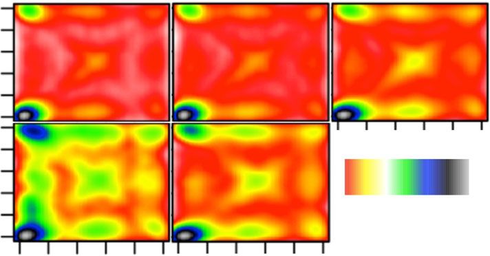
ARTICLE                                                                 NATURE COMMUNICATIONS | https://doi.org/10.1038/s41467-020-14974-x

T
       he genome is hierarchically organized in three-dimensional             matrix and constructs a Hi-C interaction graph, where each node
       (3D) space1, and chromosomal sequences can be mapped                   on the graph represents a genomic bin. If two bins are interacting,
       to one of two major compartments: compartment A is                     an edge connecting them is added to the graph, and the weight of
associated with open chromatin, and compartment B is associated               the edge corresponds to the normalized Hi-C sequencing read
with closed chromatin. The A/B compartments are predicted                     count between the two bins. Then, SCI uses graph embedding8 to
from chromatin interaction data, in particular, data generated by             project the interaction graph into a lower-dimensional vector
the genome-wide Hi-C chromatin interaction profiling technique,                space for k-means clustering to predict sub-compartments
which combines proximity-based ligation with massively parallel               (Fig. 1a).
sequencing2. Recent studies of additional data types, including                  Specifically, SCI adapts a graph-embedding method termed
methylation, DNase I hypersensitive sites, and single-cell ATAC-              LINE8 to project an otherwise high-dimensional graph structure
seq, have corroborated the existence of A/B compartments as                   into a lower-dimensional space that describes the chromatin
functional units of genome organization3. The genome can be                   interactions. LINE utilizes first-order and second-order proximi-
further subdivided into sub-compartments, where genomic                       ties of graph vertices to reduce dimensionality and promote
regions within a given sub-compartment are more likely to                     efficient clustering.
interact with each other than with regions in different sub-                     The number of sub-compartments in the nucleus is jointly
compartments. Subsequent to the A/B compartment model, a                      determined by (a) the spatial location of chromatin and (b)
three-sub-compartment model was introduced based on higher-                   chromatin interactions. Importantly, local epigenetic status can
resolution Hi-C inter-chromosomal interaction data4: one sub-                 impact chromatin interactions9. Using gap statistics to determine
compartment is a component of the open chromatin compart-                     the optimal number of sub-compartments, we obtained nine as
ment; and the other two sub-compartments are components of                    the optimal number of sub-compartments (named C1–C9).
closed chromatin compartment, one near centromeres and the                    However, some of these sub-compartments are enriched for
other far from centromeres. The latest model proposes five sub-                similar epigenetic modifications (C3 and C4; C5 and C6),
compartments based on the use of hidden Markov modeling                       suggesting that sub-compartments can be spatially separated
(HMM) to cluster inter-chromosomal interactions5. This method                 and functionally comparable—they still show comparable levels
identifies two active sub-compartments (A1 and A2) and three                   of transcriptional potential (Supplementary Fig. 1). To allow for
inactive sub-compartments (B1, B2, and B3) using deeply                       direct comparison of SCI with other computational methods for
sequenced GM12878 cell line data. The model also shows that the               predicting sub-compartments, we chose to use 5 clusters in
five sub-compartments exhibit distinct epigenomic signatures.                  subsequent SCI performance evaluations. Importantly, SCI offers
Since sub-compartments are essential for understanding higher-                users the flexibility to select the number of sub-compartments
order 3D genome organization, and an increasing volume of                     based on either their preference or the optimal number calculated
genome-wide chromatin interaction data will soon be available                 by gap statistics.
through the ENCODE and 4D Nucleome consortia, there is a                         We then assessed the performance of SCI based on structural
practical need for an easy-to-use, automated, and accurate sub-               and functional evaluations (Fig. 1b). We also developed a deep
compartment predictor.                                                        neural network classifier for predicting sub-compartments using
   In addition to Hi-C, other types of genome-wide sequencing                 DNA sequencing data and epigenomic profiles (Fig. 1b).
data have been used to predict the higher-order genome organi-
zation. For example, chromatin immunoprecipitation sequencing
(ChIP-seq) data of 11 histone modifications and 73 transcription               SCI outperforms alternative algorithms. We compared sub-
factors (TFs) have been used to predict sub-compartments with                 compartments predicted by SCI to those predicted by HMM
63% test accuracy using a deep learning multi-class classifier6.               (reported in Rao et al. 2014) and by k-means clustering applied
Recently, TSA-Seq, a new genome-wide mapping method that                      directly to an inter-chromosomal interaction matrix (Kmean-
estimates mean distances of chromosomal loci from nuclear                     s_Yaffe, reported in Yaffe, E. and Tanay, A., 2011). We tested
structures, was used to predict several Mbp chromosome trajec-                each algorithm using data from Rao et al., who generated 4.9
tories between nuclear structures7. These findings use sub-                    billion Hi-C reads from GM12878, a human lymphoblastoid
compartment assignments either for predictive model output                    ENCODE cell line.
labels or for evaluation of the distances between nuclear speckles.              When given the same parameter (k = 5), SCI predicted
These studies require accurate sub-compartment determination.                 comparable number of sub-compartments as that predicted by
Also, a DNA methylation correlation matrix based on multiple                  HMM (C1-C5; Fig. 1c, Supplementary Fig. 3); however,
replicates corroborates the A/B compartment model3. However,                  Kmeans_Yaffe failed to predict five sub-compartments, as it
the potential of DNA methylation levels to predict nuclear sub-               placed genomic bins in four sub-compartments instead of 5
compartmentalization is still not clear.                                      (Supplementary Fig. 2). Following the convention of Rao et al., we
   Here, we introduce SCI, an algorithmic framework based on                  reordered sub-compartments predicted by SCI such that
graph embedding8 and k-means clustering that predicts genomic                 sub-compartments C1 and C2 correspond to open chromatin
sub-compartments from Hi-C data. We show that sub-                            sub-compartments reported by Rao et al. (A1 and A2), while sub-
compartment prediction by SCI is more accurate than other                     compartments C3, C4, and C5 correspond to closed chromatin
unsupervised algorithms. Furthermore, we use orthogonal data                  sub-compartments reported by Rao et al. (B1, B2, and B3). Sub-
for external validation, including ChIA-PET chromatin interac-                compartments C1 and C2 have higher gene density compared to
tion, transcriptome, and epigenome data. Lastly, using SCI out-               the other three sub-compartments (Fig. 1d), which is consistent
put, we developed an epigenome-based (DNA methylation and                     with the previous reports10.
histone modification) deep neural network model for sub-                          Our UMAP visualization of SCI embedding (Fig. 1e) shows: (i)
compartment classification.                                                    a clear distinction between sub-compartments C1 (in red) and C2
                                                                              (in yellow), which was indirectly reported in the literature
                                                                              by measuring the distance from lamina-associated domains
Results                                                                       (LADs)11; and (ii), clear separation of the inactive sub-
SCI overview. To predict sub-compartments, SCI starts with a                  compartment C3 (in gray) from the inactive sub-compartments
normalized, genome-wide Hi-C inter-chromosomal contact                        C4 (in purple) and C5 (in blue). We further showed that the open

2                NATURE COMMUNICATIONS | (2020)11:1173 | https://doi.org/10.1038/s41467-020-14974-x | www.nature.com/naturecommunications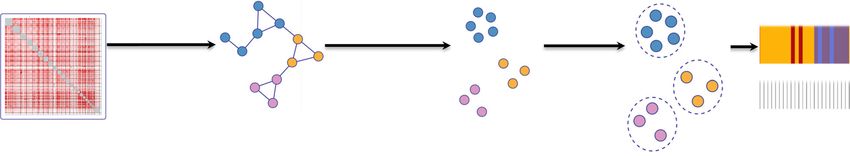
NATURE COMMUNICATIONS | https://doi.org/10.1038/s41467-020-14974-x ARTICLE
a Hi-C interaction Low-dim Sub-compartment Visualization
Genomic bins
graph Graph vector space
C1 Sub-
Embedding
Filtering low Kmeans compartments
coverage bins clustering
C2
1st order
proximities Genomic bins
+ C3
2nd order
proximities
b c d
C1 9000 8 Active
Structural evaluation
C2
C3
Gene density
Functional evaluation
Bins count
4500 4
Inactive
Deep learning classifier
DNA sequence
+
0 0
Epigenomic profile
C1 C2 C3 C4 C5 C1 C2 C3 C4 C5
e f 3.0 g
Active
Open
C1 C1 2.5
ATAC-seq enrichment
10 10 C2 10
C1 2.0
ive C5
In act
Dim 2
Dim 2
Dim 2
0 0 C3 0
C5 1.5
1.0 C5
–10 C3 –10 –10 C4
Close 0.5 NAD
C4
–10 –5 0 5 10 –10 –5 0 5 10 0.0 –10 –5 0 5 10
Dim 1 Dim 1 Dim 1
h i j k
1.2 20 0.5
log2 Betwenness centrality
0.4 SCI
1.0
Closeness centrality
Clustering coeficient
17.5
0.3
0.8
15 HMM
0.2
0.6
12.5 0.1
Random
0.4
0
SCI HMM SCI HMM SCI HMM –0.25 0.00
Silhouette index
Fig. 1 SCI utilizes a chromatin interaction graph to predict genomic sub-compartments. a The SCI workflow starts with a normalized Hi-C inter-
chromosome matrix. From this matrix, the interaction graph is constructed; nodes with the same color represent bins from the same chromosome. After
building the interaction graph, the graph embedding step transforms the graph into a lower-dimensional space. Finally, k-means clustering is used to cluster
node representations. b SCI-predicted sub-compartments are validated using structural and functional properties and serve as class labels to train a sub-
compartment classifier based on a feature matrix compiled with features of DNA sequence and epigenomic profiles (methylation and histone
modifications), and replication timing data. c Bar plot of genomic bin count for each sub-compartment. d Bar plot of gene density measured as the number
of genes per genomic bin for each sub-compartment. Sub-compartments associated with open chromatin (C1 and C2) show higher gene density compared
to sub-compartments associated with closed chromatin (C3-C5). e UMAP 2-D projection of SCI’s embedding with 100 dimensions showing clustered sub-
compartments for GM12878 Hi-C data. f ATAC-seq enrichment evaluating open and closed chromatin states across all five sub-compartments.
g Distribution of nucleolar-associating domains (NADs) between C4 and C5. h–k Comparison of clustering quality metrics between SCI and HMM:
(h) closeness centrality, (i) betweenness centrality, (j) clustering coefficient and (k) Silhouette index. For the boxplots, the top and bottom lines of each
box represent the 75th and 25th percentiles of the samples, respectively. The line inside each box represents the median of the samples. The upper and
lower lines above and below the boxes are the whiskers. Asterisks (***) represent p-values < 2.2e−16 using Mann–Whitney test.
NATURE COMMUNICATIONS | (2020)11:1173 | https://doi.org/10.1038/s41467-020-14974-x | www.nature.com/naturecommunications 3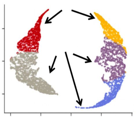
ARTICLE                                                                 NATURE COMMUNICATIONS | https://doi.org/10.1038/s41467-020-14974-x

chromatin-associated sub-compartments (C1 and C2) have higher                 Supplementary Fig. 6) than CTCF ChIA-PET inter-loops. SCI-
enrichment of ATAC-seq compared to the inactive compartments                  detected sub-compartments achieved a higher intra-loop vs. inter-
(Fig. 1f, open-chromatin sub-compartment C1 compared to                       loop ratio of normalized CTCF ChIA-PET loop counts compared
closed-chromatin sub-compartment C3, and open-chromatin                       to HMM-detected sub-compartments (Fig. 2c, p-value < 2.2 ×
sub-compartment C2 compared to closed-chromatin sub-com-                      10−16, Fisher’s exact test). RNAPII ChIA-PET data corroborated a
partment C5). Moreover, we show that C4 is more highly enriched               higher ratio of intra-loops vs. inter-loops using SCI compared to
for nucleolar-associating chromosomal domains (NADs)12 com-                   HMM (Fig. 2d–f). This equated to a 60% and 74% more robust
pared to C5 (Fig. 1g), indicating that C4 is located in the nucleolus         performance for SCI compared to HMM for CTCF and RNAPII
while C5 is likely not. Thus, SCI-predicted sub-compartments                  loop ratios, respectively. We then visualized the ChIA-PET loops
exhibit distinct chromatin characteristics.                                   in an example region with more intra-loops than inter-loops
   Genomic regions that map to the same sub-compartment                       (Fig. 2g). Together, these data demonstrate that, compared to
based on the graph embedding of SCI are expected to be in                     HMM-prediction of sub-compartments, SCI-prediction of sub-
proximity to each other in 3D space. To test this, we examined                compartments achieves better clustering performance and tighter
intra-sub-compartment, inter-chromosomal chromatin interac-                   network topology structure.
tion network topology features, including network centrality
(closeness and betweenness) and the clustering coefficient.
Compared to the HMM approach, SCI showed significantly                         Functional assessment of sub-compartments. To compare the
higher closeness centrality (p-values < 2.2e−16, Mann–Whitney                 functional properties of sub-compartments predicted by SCI with
test) and betweenness centrality, and a higher graph clustering               those of sub-compartments predicted by other methods, we
coefficient within sub-compartments (Fig. 1h–j), with improve-                 assessed enrichment for epigenomic marks and replication timing
ments between 8–10%. In addition, we found that open sub-                     within sub-compartments. Data comprised DNase hypersensitive
compartments (C1 and C2) show higher centrality values for                    sites (DHS) (open chromatin), ten histone modifications,
chromatin interactions compared to the closed sub-                            enhancer annotations, super-enhancer annotations, DNA
compartments (C3, C4, C5) (Supplementary Fig. 3), indicating                  methylation, and six replication timing datasets (Fig. 3a, Sup-
that heterochromatin is more spatially constrained than euchro-               plementary Fig. 7). In general, transcriptionally active sub-
matin. These topological network features indicate higher                     compartments are expected to have higher enrichment for DHS
chromatin interactions between genomic regions within the same                and the histone modifications (H3K27ac and H3K36me), com-
SCI-predicted sub-compartments. To further evaluate the cluster-              pared to transcriptionally inactive sub-compartments. While
ing performance of SCI and HMM, we calculated their Silhouette                inactive sub-compartments are expected to have higher enrich-
indices, which measure the consistency within clusters of data13.             ment for H3K27me3 and DNA methylation. We found that SCI-
The Silhouette index ranges from −1 to 1, where a higher value                predicted sub-compartments satisfied these expectations (Fig. 3a).
indicates better clustering performance. SCI improved the                     In contrast, HMM-predicted sub-compartments exhibited higher
Silhouette index over the previous HMM sub-compartment                        enrichment for DHS in C3 (inactive) than in C2 (active) (Sup-
annotation by 8% (Fig. 1k). Moreover, we calculated the Davies-               plementary Fig. 7). We observed higher enrichment for enhancers
Bouldin index, where lower values are better, and SCI improved                and super-enhancers in the C1 and C2 sub-compartments pre-
the Davies-Bouldin index by 7% (Supplementary Fig. 4). We also                dicted by both SCI and HMM (Fig. 3a, Supplementary Fig. 7),
compared LINE to the state-of-the-art graph embedding algo-                   consistent with transcriptionally active genomic regions.
rithms HOPE14 and DeepWalk15. LINE-based cluster results had                     Genes in close 3D spatial proximity to one another are more
a better Silhouette index and centrality measures compared to the             likely to have synchronized transcriptional control compared to
alternative graph embedding methods (Supplementary Fig. 5).                   those that are in different sub-compartments18. Therefore, we
                                                                              examined transcriptional activity in SCI-predicted sub-compart-
                                                                              ments. We assessed gene-expression levels using ENCODE RNA-
SCI performance validated with ChIA-PET data. To further                      seq data of GM12878 cells. Genes within C1 and C2 had
validate that genomic regions from any given Hi-C-based SCI-                  significantly higher transcript per million (TPM) values (p-value <
predicted sub-compartment have higher chromatin interaction                   0.01 based on ANOVA) compared to genes within C3-5,
frequencies than those from different sub-compartments, we                    consistent with their epigenetic regulatory status (Fig. 3b).
applied SCI to datasets from an orthogonal chromatin interac-                 Furthermore, we evaluated the generation of nascent RNA using
tion assay, Chromatin Interaction Analysis by Paired-End Tag                  Global run-on sequencing (GRO-seq)19. The GRO-seq data
Sequencing (ChIA-PET). ChIA-PET measures chromatin                            confirmed that transcriptional activity in C1 and C2 is
interactions associated with specific protein factors16. We used               significantly higher (fold change > 3, p-value < 0.01 based on
two different ChIA-PET datasets: the first captures interactions               ANOVA) than that in sub-compartments C3-5 (Fig. 3c).
associated with CCCTC-binding factor (CTCF), a chromatin-                        We hypothesize that the expression of genes within the same
binding protein associated with more than 70% of the total                    sub-compartment is more highly coordinated than that of genes
chromatin interactions17; and the second captures interactions                across different sub-compartments. Therefore, we calculated
associated with RNA polymerase II (RNAPII), which coordi-                     pairwise Spearman’s correlation of gene expression for gene pairs
nates communication between promoters and their distal reg-                   within the same sub-compartment and across sub-compartments.
ulatory elements. We then compared the chromatin interactions                 We observed higher pairwise correlation values of gene expres-
in GM12878 cells measured by CTCF and RNAPII ChIA-PET to                      sion for genes falling into bins within the same sub-compartment
quantify two types of chromatin interactions: (i) intra-loops,                (intra-compartment correlation) compared to genes in different
which are defined as ChIA-PET chromatin loops that connect                     sub-compartments (inter-compartment correlation) (Fig. 3d). We
two genomic bins that have the same sub-compartment pre-                      also showed that SCI achieved a significantly higher (P-value <
dictions; and (ii) inter-loops, which are defined as ChIA-PET                  2.2e−16, paired Wilcoxon test) intra-compartment correlation to
chromatin loops that connect two genomic bins that have dif-                  the inter-compartment correlation ratio compared to HMM. As
ferent sub-compartment predictions (Fig. 2). We showed                        shown in Fig. 3e, SCI performs 40% better than HMM with
that there are more CTCF ChIA-PET intra-loops (the diagonal                   respect to pairwise gene-expression correlation for functional
of the heatmap in Fig. 2a and the top panel of Fig. 2b and                    evaluation of sub-compartments.

4                NATURE COMMUNICATIONS | (2020)11:1173 | https://doi.org/10.1038/s41467-020-14974-x | www.nature.com/naturecommunications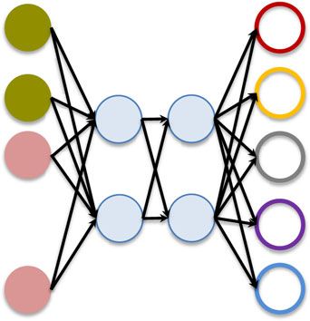
NATURE COMMUNICATIONS | https://doi.org/10.1038/s41467-020-14974-x ARTICLE
CTCF ChIA-PET data validation
a b c Intra- vs. inter-loops
17.5
17 4 3 1 3 C1 2.0 ***
Normalized loop count
15.0
Ratio of loop count
15
4 14 3 2 6 12.5
C2 Intra- 1.5
loop 10.0
3 3 5 1 1 C3 7.5 1.0
10
5.0
1 2 1 3 2 C4
2.5 0.5
3 6 1 2 9 C5 0.0
5 C1 C2 C3 C4 C5 0.0
0.0
C1
C2
C3
C4
C5
Inter- –2.5 All C1 C2 C3 C4 C5
loop –5.0
Subcompartment
RNA Pol II ChIA-PET data validation
d e f Intra- vs. inter-loops
30.0 4 ***
Ratio of loop count
29 4 2 1 0 C1 Intra-loops: Loops anchor in the
SCI HMM
25.0 genomic bins from the same type
Normalized loop count
25 3
4 26 3 2 2 C2 Intra- 20.0 of sub-compartment.
20 loop 2
2 3 4 0 0 C3 15.0 Inter-loops: Loops anchor in the
genomic bins from the different type
15 10.0 1
1 2 0 3 2 C4 of sub-compartment.
5.0 0
0 2 0 2 4 C5 10
0.0
C1 C2 C3 C4 C5 All C1 C2 C3 C4 C5
C1
C2
C3
C4
C5
5 Inter- 0.0 Subcompartment
loop
–50
g
chr11:107356150–109739196
Hi-C
Compartment B A B
Sub-compartment C2 C1 C2 C1 C2 C5 C4 C5 C4 C5
Genomic bin 100
CTCF n = 76
10
Intra-loops 0
100
CTCF n=7
10
Inter-loops 0
RNA Pol II n = 27 10
3
Intra-loops
0
RNA Pol II n=6 10
3
Intra-loops
0
10
RNA-seq
5
0
ELMOO1 SLN SLC35F2 CUL5 ACAT1 ATM C11orf65 EXPH5 DDX10 AP11-2519.2 RNA5SP349 RP11-708B6.2 RP11-262A12.1
ELMOO1 SLN SLC35F2 CUL5 ACAT1 ATM EXPH5 DDX10 U6 SNORD39 RP11-708B6.2
Gencode ELMOO1 SLN AP001024.2 RAB39A CUL5 ACAT1 ATM EXPH5 DDX10 DDX10 DDX10 C11orf87
ELMOO1 AP001024.1 ACAT1 ATM C11orf65 EXPH5 DDX10
ELMOO1 SLC35F2 ACAT1 ATM C11orf65 EXPH5 DDX10
ALKBH8 ELMOO1 SLC35F2 ACAT1 ATM C11orf65 EXPH5 DDX10
Fig. 2 External validation of SCI-predicted sub-compartments using orthogonal ChIA-PET chromatin interaction data. Validation using CTCF ChIA-PET
(a–c) and RNAPII ChIA-PET (d–f). a, d Heatmaps of ChIA-PET loop counts per predicted sub-compartment, based on the mapping of loop anchors to
genomic bins. Loop counts normalized genome-wide using sub-compartments determined by SCI. b, e Plots visualizing the abundance of ChIA-PET loops
across SCI-predicted sub-compartments. c, f Bar plots comparing the ratios of ChIA-PET loops connecting genomic bins within the same sub-
compartments to the loops connecting genomic bins from different sub-compartments, based on the sub-compartment predictions by SCI and HMM.
g Example regions of SCI sub-compartment predictions that have more intra-sub-compartment loops (intra-loops) than inter-sub-compartment loops
(inter-loops) supported by CTCF and RNAPII ChIA-PET. Asterisks (***) represent p-value < 2.2 × 10⁻¹⁶ using Fisher’s exact test.
Folding the genome into sub-compartments may optimize the BRCA1 TFs. We found that ChIP-seq-based TF enrichment
efficient usage of transcriptional regulatory elements. If true, we patterns agree with the predicted sub-compartment-specific TFs,
would expect to see sub-compartment-specific TF enrichment. To where MYC and BRCA1 are enriched in C1, and BATF and
test this, we assessed TF enrichment using elastic net regression, EP300 are enriched in C2 (Fig. 4c). In addition, we observed that
which infers the regulatory elements that control transcription for YY1, a TF common to both C1 and C2, is not enriched in either
each sub-compartment20. Based on feature dependency analysis20 sub-compartment. These results indicate that SCI can identify
(see Methods section for details), we identified sub-compartment- chromatin hierarchical sub-compartments that parse into tran-
specific TFs that can be used to predict gene-expression levels in scriptional regulatory units.
each sub-compartment (Supplementary Table 1). We also
identified sub-compartment-specific TFs (red text in Fig. 4a, b).
To further validate C1- and C2-specific TFs, we evaluated Deep neural network for predicting sub-compartments. Recently,
ENCODE ChIP-seq data that was available for MYC, EP300, and models have been proposed for predicting sub-compartment-level
NATURE COMMUNICATIONS | (2020)11:1173 | https://doi.org/10.1038/s41467-020-14974-x | www.nature.com/naturecommunications 5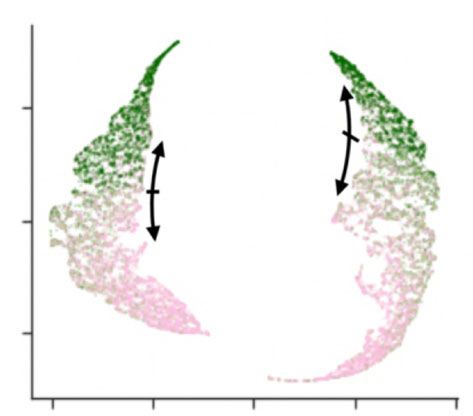
ARTICLE NATURE COMMUNICATIONS | https://doi.org/10.1038/s41467-020-14974-x
a b d
2.5 0.4
DHS 1.8 1.5 1.1 0.8 0.6 Intra-sub-compartment ρ
Spearman correlation
H3K36me3 3.3 2.5 1.0 0.9 0.9 2.0 Intra-sub-compartment ρ
0.3
H3K27me3 0.9 1.0 1.4 1.0 0.8
1.5
H3K9me3 1.1 1.2 1.1 0.9 0.8
TPM
H4K20me1 1.4 1.3 1.1 0.8 0.7 0.2
1.0
H2az 1.6 1.5 1.0 0.9 0.8
H3K27ac 4.1 3.2 1.1 0.7 0.7 4 0.5 0.1
H3K4me1 2.4 2.1 1.1 0.7 0.6
0
H3K4me2 3.5 2.8 1.1 0.7 0.6 0.0
Fold change
C1 C2 C3 C4 C5 0.0 0.5 1.0
H3K4me3 2.0 1.7 1.0 0.9 0.8 1e7
Distance
H3K79me2 7.2 4.3 1.0 0.8 0.7 1
H3K9ac 2.5 1.9 1.0 0.9 0.8 c e Intra-sub-compartment ρ
Ratio =
RepG1 8.3 5.8 1.1 0.6 0.5 Inter-sub-compartment ρ
6
RepS1 3.1 2.9 1.2 0.2 0.1 C1 4.0
C2 ***
RepS2 0.9 1.5 2.1 0.6 0.2
0.25 3.5
Correlation ratio
Gro-seq singal
RepS3 0.1 0.2 2.2 1.9 0.9 4 C3
C4 3.0
RepS4 0.2 0.2 0.8 3.0 3.4
C5
RepG2 0.9 0.8 0.6 2.1 6.7 2.5
2
Enhancers 2.2 1.8 0.9 0.4 0.2
2.0 SCI
Super Enhancers 3.1 2.6 0.1 0.1 0.1
Rao_HMM
Methylation 0.7 0.8 1.0 1.2 1.2 1.5
0
C1 C2 C3 C4 C5 –400 TSS +400 0.0 0.5 1.0
Position Distance 1e7
Fig. 3 SCI sub-compartments have distinct genomic features. a Heatmap of distinct epigenomic sub-compartments predicted by SCI. b Boxplot of gene
expression in transcripts per million (TPM) for different compartments. C1 and C2 have higher gene expression compared to other sub-compartments.
c Cumulative GRO-seq signal over the promoter regions for all the genes in each sub-compartment. d Pairwise gene-expression Spearman’s correlations
vs. distance between gene pairs within the same sub-compartment (in black) vs. gene pairs across sub-compartments (gray) within 10 Mbps.
e Spearman’s correlation coefficient ratio (y-axis) of gene pairs within the same sub-compartment (in black) vs. gene pairs across sub-compartments
plotted against genome distance (x-axis) for SCI (blue) and HMM prediction. Asterisks (***) represent p-value < 2.2e−16 using paired Wilcoxon test.
a YY1
b YY1
c 3
C1 regulators 0.06 C2 regulators
Fold change
ELK1 1.71
C1 3.13 3.04 2.31 2.08
0.03
Aggregate error changes
Aggregate error changes
0.05 2.4
C2 2.09 2.03 2.84 2.54 1.94
0.04 2
0.02
1
1
ELF5 0
YC
TF
YY
CA
30
0.03
BA
M
EP
BR
ARNT
ETV6
MYC 0.02
0.01 ELK1
SPIB ZBTB7B
BRCA1 E2F2
E2F5 0.01 BATF
EP300
0.00 0.00
0 100 200 300 400 500 600 0 100 200 300 400 500 600
Regulators Regulators
Fig. 4 Sub-compartment-specific transcription factor prediction. a–b Scatter plot showing sub-compartment-specific transcription factors (TFs)
participating in transcriptional regulation predicted by elastic net regression for C1 and C2 sub-compartment. The star indicates TFs with the ChIP-seq data
available from ENCODE (red: C1-specific regulators, orange: C2-specific regulator, and gray: shared regulator). c Heatmap of ChIP-seq enrichment for
MYC, BRCA1, BATF, EP300, and YY1 TFs across sub-compartments.
genome structure from the DNA sequence, ChIP-seq data6, and (Fig. 5a). Building on these distinctions, we developed an
other 3D genome assays7. One approach uses a 450 K-based DNA epigenome-based classifier to predict sub-compartments based
methylation correlation matrix from multiple replicates (n ≥ 62) to on ChIP-seq epigenomic marks and whole-genome bisulfite
identify genome-wide A/B compartments. However, there is no sequencing data, using a deep neural network (DNN) (Fig. 5b).
available model for sub-compartment structure prediction using a We combined dynamic epigenomic features and static DNA
single DNA methylation library. sequence features to design a deep neural network (DNN). We
Using SCI predictions, the five sub-compartments showed sliced the data set into a training set (80%) and test set (20%). The
distinct epigenome signatures (Fig. 3a), DNA methylation model accuracy reached higher test accuracy (0.73) using SCI-
percentage distributions, and percentage of disordered reads, detected class labels than using HMM-detected class labels (0.68)
the latter of which is a measurement of epigenome stochasticity21 or using randomized class labels (0.23) with the same class sizes
6 NATURE COMMUNICATIONS | (2020)11:1173 | https://doi.org/10.1038/s41467-020-14974-x | www.nature.com/naturecommunications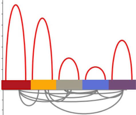
NATURE COMMUNICATIONS | https://doi.org/10.1038/s41467-020-14974-x ARTICLE
a b
100 Static features:
Input Output
C1 C2 C3
layer layer
DNA Sequence
DNA methylation %
1. 2-mer count C1
Sub-compartments
2. 3-mer count … Hidden layers
0 C2
100 Dynamic features:
C4 C5 0 1
DNA Methylation information: C3
… …
1. Methylation (% distribution,
PDR distribution,
Low High Epipolymorphisim … C4
0 distribution)
Density
2. Histone modification ChIP-
0 10 1 seq data and replication
C5
timing data
Disordered methylation
c
compartment
output labels
Random labels
MLP sub-
HMM labels
SCI labels
0.2 0.4 0.6 0.75
Test accuracy
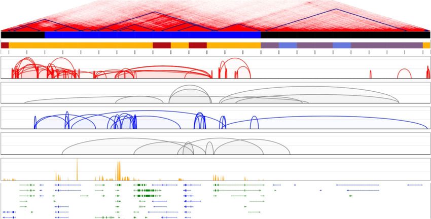
Fig. 5 Deep neural network predicting sub-compartments using DNA methylation. a Smoothed scatter plot showing the distribution of the percentage of
DNA methylation and the proportion of disordered DNA methylation reads for all sub-compartments. b The schematic diagram for the constructed a deep
neural network (DNN) model to predict sub-compartments from methylation and DNA sequence features. c Bar plot showing the accuracy of sub-
compartment prediction using random classifier trained with random labels, HMM sub-compartment annotation, or SCI sub-compartment annotation.
(Fig. 5c). In addition, we developed a more compact model using Discussion
only DNA methylation and DNA based features, which was able Hi-C enables the elucidation of higher-order chromatin topology
to predict genomic sub-compartments with 0.66 of accuracy. that suggests structural regulation of transcriptional control.
Because the model interpretability of DNN is limited, we used a Software exists for data pre-processing, chromatin loop calling,
gradient-boosted trees model (XGBoost) classifier and random and topologically associating domain (TAD) predictions. How-
forest machine learning methods to derive a feature importance ever, there is no available software to examine compartment and
score for our features. The accuracy of the XGBoost classifier is sub-compartment structures. Furthermore, it has been shown
0.69, and the accuracy of the random forest method is 0.67, each that the TAD structure is rather stable among different cell types,
of which is slightly lower than the accuracy of our DNN model. while the structure of sub-compartments is highly variable among
The XGBoost and random forest methods agreed that histone different cell types; this validates the need to study the cell type-
modification features followed by DNA methylation distribution specific functions of sub-compartments22. SCI identifies complex
are the most important feature in the dataset (Supplementary nuclear sub-compartments in a fully data-driven, unsupervised
Fig. 8). fashion.
Our sub-compartment DNN predictors outperformed recently In contrast to previous methods that infer sub-compartments
developed model6 using 84 ChIP-seq libraries for histone modifica- using HMM, SCI more comprehensively utilizes network prop-
tions and TFs using the same training/test data split (training data erties and thus may preserve the global structure of the chromatin
is from odd-numbered chromosomes and test data is from even- interaction network. SCI formulates sub-compartment prediction
numbered chromosomes) (Supplementary Table 2). Moreover, as a graph-based problem and enables efficient utilization of Hi-C
our reduced model using DNA methylation and DNA features information via graph embedding. SCI considers both the first-
outperformed their reduced model using 11 histone marks. order and second-order proximities, which complement the
sparsity of first-order proximity in Hi-C data. We demonstrated
that SCI outperforms other algorithms, such as HMM and
Compartment prediction using Hi-C or ChIA-PET data. We Kmeans_Yaffe. We believe that the superior performance of SCI
also used SCI to predict A/B compartments from Hi-C and compared to other methods is due to its use of all the inter-
ChIA-PET data on two cell lines: GM128787 (human B-lym- chromosomal interactions, and efficient dimensionality reduction
phocyte) and K562 (human lymphoblast). We predicted A/B via graph embedding. Specifically, Rao_HMM uses only a subset
compartments using a 100-kb resolution. We observed high of inter-chromosome interactions, and Kmeans_Yaffe does not
agreement for A/B compartment prediction from both technol- perform a dimensionality reduction on the data. Importantly, we
ogies (Supplementary Fig. 9) (agreement for GM12878 is 91% studied the functional relevance of sub-compartments as they
and agreement for K562 is 78%). We observed a high correlation relate to cellular processes. Moreover, we show TF enrichment in
(0.88 for GM12878 and 0.76 for K562) for the first eigenvector SCI-predicted sub-compartments.
values between Hi-C and ChIA-PET. Moreover, we noted that Recently, various computational models have been proposed to
enrichment for several open chromatin marks, histone marks, predict genome organization from sequence and epigenomic
and replication timing data was similar using compartments data6 and other 3D genome assays7. We believe that SCI will
called by Hi-C and ChIA-PET for both cell lines (Supplementary further propel the development of such models by providing
Fig. 10). We implemented the compartment predictor using robust, accurate labels for genomic sub-compartments. As an
static features (DNA sequence information) and dynamic fea- example, we developed compartment and sub-compartment
tures (DNA methylation information) as input for the deep DNN predictors using static features from the DNA sequence
neural network model and achieved 87% test accuracy (Supple- of the reference genome and dynamic features from histone
mentary Fig. 11). modifications and DNA methylation data and outperformed the
NATURE COMMUNICATIONS | (2020)11:1173 | https://doi.org/10.1038/s41467-020-14974-x | www.nature.com/naturecommunications 7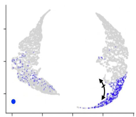
ARTICLE                                                                          NATURE COMMUNICATIONS | https://doi.org/10.1038/s41467-020-14974-x

published model6 using 84 ENCODE ChIP-seq libraries for his-                          considered as a simple vertex or as a context to other vertices. LINE introduces two
tone modifications and TFs from the same cell line.                                    vectors ui and u0i , where ui is the representation for vi as a vertex while u0i is the
                                                                                      representation for vi as a context.
   Importantly, the ENCODE and 4D Nucleome consortia are                                 For each directed edge in the graph (i, j) (undirected edges are treated as two
generating robust Hi-C datasets, and we anticipate that SCI will                      directed edges with opposite directions), LINE defines the probability of context vj
contribute to more efficient and accurate sub-compartment                              generated by vertex vi as:
determination, and will improve our understanding of the com-
                                                                                                                                exp u0 Tj  ui
plex interactions between DNA methylation, gene expression,                                                      p2 vj jvi ¼ P             T                             ð3Þ
                                                                                                                                             0
and chromatin organization. Furthermore, tens of thousands of                                                                    k2V exp u k  ui
DNA methylation assays have been generated in large-scale stu-                                                                           w
                                                                                      Empirical distribution ^p2 is defined as ^p2 ¼ dij , where di is the out-degree of node i.
dies such as The Cancer Genome Atlas, the Epigenome Roadmap,                                                                          i
                                                                                         LINE optimizes scaled (scaled by node degree) versions of the KL divergence
and Cancer Cell Line Encyclopedia. SCI will provide methods to                        between p2 and ^p2 . It defines
maximize the value of these datasets and thereby enrich our                                                              X
                                                                                                                 O2 ¼         wij log p2 vj jvi                           ð4Þ
understanding of the layers of gene-expression coordination that                                                          wij 2E
are important for development and disease states.
                                                                                         SCI implements two approaches to combine defined objective functions O1 and
                                                                                      O2. In the first approach, SCI optimizes O1 and O2 independently and then
Methods                                                                               combines representation from both orders into a final representation. In the second
Background. All current sub-compartment prediction methods utilize an inter-          approach (joint optimization), SCI combines first-order and second-order
chromosomal interaction matrix to predict sub-compartments. Two methods for           proximity objective functions into one function to define O3 as:
prediction of genomic sub-compartments have been published. First model is the
                                                                                                                O3 ¼ ð1  αÞO1 þ αO2 ; α 2 ½0; 1                          ð5Þ
Yaffee and Tanay sub-compartment model (Yaffee_Kmeans). This model applies
K-means clustering directly on a HiC interaction matrix. It modifies the distance      where α is a mixing parameter to determine the weight of first-order and second-
calculation method such that it ignores all distance computation that involves        order optimization functions.
intra-chromosomes entries. This model identifies three sub-compartments: one              It then optimizes both orders at the same time. An asynchronous gradient
active and two inactive sub-compartments. The second model is Rao sub-                descent algorithm coupled with negative sampling is used to optimize all objective
compartments (HMM). The Rao sub-compartment prediction method focuses on              functions. The joint optimization showed a 30% increase in time efficiency (from
one sub-set of inter-chromosomal interactions: the interactions between odd-          26 min to 18 min using GM12878 Hi-C data) and a slightly lower clustering
numbered and even-numbered chromosomes. This method uses HMM to cluster               performance of the joint optimization compared to separate optimization
the interactions between odd-numbered and even-numbered chromosomes in                (measured by Silhouette index, Davies-Bouldin index, and centrality measures,
different runs. After performing cluster annotation for odd-numbered and even-        Supplementary Fig. 12). Both separate and joint optimization are available as
numbered chromosomes, the Rao method combines those annotations into a single         options in the SCI code.
final cluster annotation based on enriched HiC interactions between the clusters of
odd-numbered and even-numbered chromosomes.
                                                                                      Evaluation for clustering methods. For each genomic bin we define Silhouette
                                                                                      index (si) as:
Graph-embedding methods. Given an undirected graph G = [V, E], where V
represents genomic bins, and E represents Hi-C interactions, each edge (e) between                                                  bi  ai
                                                                                                                          si ¼                                             ð6Þ
vi and vj has weight wij, which represents the normalized Hi-C read count. Graph-                                                  maxðbi ; ai Þ
embedding approaches project graph G into a low dimension space Rd by calcu-          where bi is the lowest average distance for genomic bin i for all other clusters, and
lating embedding matrix U (please refer to the following reviews for more detailed    ai is the average distance from genomic bin i from all points in the same cluster.
information about graph embedding23–25). We compared SCI graph embedding                  We used the silhouette_score function from scikit-learn package version 0.19.2.
method to DeepWalk and HOPE graph embedding methods.                                  We used Euclidean distance as our distance measure.
    The Deepwalk method relies on performing random walks across the graph that           The Davies–Bouldin index (DBI) is defined as:
have a specific length. These walks resemble node sequences in the graph, and this
sequence is fed to the Word2Vec approach to derive the embedding of the graph                                                     1X k

vertices based on their context. The original DeepWalk implementation handles                                         DBI ¼             maxi≠j Dij                         ð7Þ
                                                                                                                                  k i¼1
only unweighted graphs. We used a modified version of the algorithm to handle
weighted graphs from (https://github.com/dongguosheng/deepwalk).                      where
    The HOPE method derives the graph embedding matrix U, which minimizes
                                                                                                                                      di þ dj
the following objective function:                                                                                          Dij ¼                                           ð8Þ
                                                                                                                                       dij
                                     S  u uT  2
                                           s t F
                                                                                          Following the definition in ref.   26,we define di and dj as the average distance
where S is a similarity matrix, and U is an embedding matrix where U = [Us, Ut].      between all pairs in clusters i and j. dij is the distance between all pairs between
The similarity matrix can be defined using different similarity measures, including    clusters i and j.
the Katz index and rooted page rank. For HOPE, we used the implementation of              The clustering coefficient is defined as the ratio of the number of closed triplets
these algorithms from the GEM graph embedding package (https://github.com/            (triangles) the node has to the number of all triplets that the node has. To adjust to
palash1992/GEM). We used Katz index similarity measures in the original               the weighted graph, the weighted average for the closed triples is calculated27.
publication14.                                                                            Closeness network centrality of a node is defined as the average length of the
                                                                                      shortest path between the node and all other nodes in the graph. Closeness
                                                                                      centrality for a node u in a graph with n nodes can be calculated as:
LINE and joint optimization. In order to project graph G into lower dimension Rd,
LINE defines two properties to preserve in the graph: first-order proximity and                                                   n1
                                                                                                                       CðuÞ ¼ Pn1                                         ð9Þ
second-order proximity.
                                                                                                                               v¼1 dðv; uÞ
   First-order proximity is defined as the pairwise proximity through edges
between the vertices in graph G. LINE models first-order proximity between two         where d(v, u) is the shortest path between nodes u and v.
vertices in graph vi and vj:                                                              Betweenness network centrality is defined as the number of times a node acts as
                                                                                      a bridge along the shortest path between two other nodes. Betweenness centrality
                                              1
                                 p1 ¼                                         ð1Þ     for a node u in a graph with n nodes can be calculated as:
                                       1 þ eui uj
                                                T

                                                                                                                             X σðs; tjuÞ
where ui and uj are vertices embedding into low-dimensional space Rd. We define                                        CB ¼                                         ð10Þ
                                                              w      P                                                            σðs; tÞ
empirical edge distribution over the space V × V, ^p1 ¼ Wij where W ¼ ði;jÞ2E wij .                                         s;t2V

To obtain the first-order embedding, LINE optimizes the KL divergence (omitting        where V is the total number of nodes in the graph. σ ðs; t Þ is the number of shortest
constants) between p1 and ^p1 as                                                      paths between nodes s and t. σðs; tjuÞ is the number of shortest paths between s and
                                    X                                                 t passing through u.
                          O1 ¼          wij logðp1 ðvi ; vj ÞÞ               ð2Þ         Closeness and betweenness centralities were calculated using NetworkX
                                   ði;jÞ2E                                            version 2.1.
   For second-order proximity, the main assumption is that vertices connected to          GM12878 CTCF and RNAPII ChIA-PET intra-chromosome loops supported
other vertices are similar. To calculate embedding based on the second-order          by at least five paired-end reads were used for loop ratio calculation. A loop anchor
proximity, LINE introduces the context concept. Each vertex in the graph is           is associated with a specific sub-compartment if it has an overlapping ratio greater

8                    NATURE COMMUNICATIONS | (2020)11:1173 | https://doi.org/10.1038/s41467-020-14974-x | www.nature.com/naturecommunications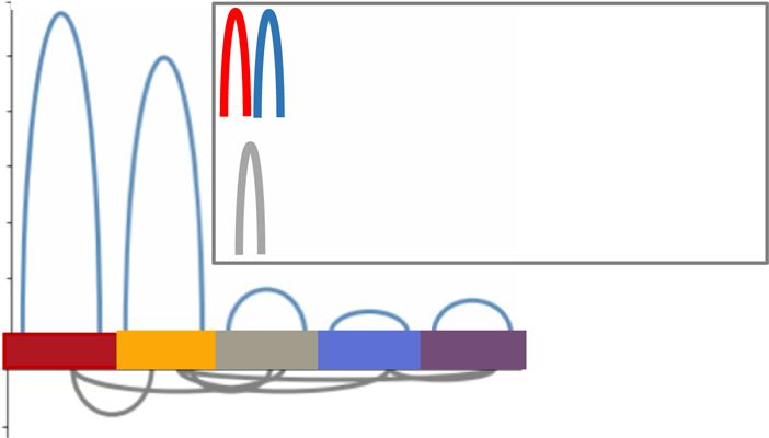
NATURE COMMUNICATIONS | https://doi.org/10.1038/s41467-020-14974-x                                                                                               ARTICLE

than 50%. Next, we create sub-compartment loop interaction matrix M (mij),                   chromatin regions, as determined by ATAC-seq data. Finally, we constructed a
where mij represents the number interaction between sub-compartments i and j                 features matrix where the genes represent samples, and all mapped TFs represent
detected using ChIA-PET data, such that the ChIA-PET loop left anchor falls in               features, and where the count of TF hits associated with a given gene represents the
sub-compartment i and the right anchor falls in sub-compartment j. As there is no            feature value. We modified the RegulatorInference tool (https://bitbucket.org/
directionality difference between the left and right anchors, we create a symmetric          leslielab/regulatorinference) to implement a sample-by-sample elastic net regres-
compartment matrix Msym as the sum of M and MT. Finally, a normalized matrix                 sion model to predict gene expression for each replicate using regulatory elements
(Mnorm) is obtained by dividing Msym by the sum of its all elements.                         in gene promoters. We optimized the elastic net mixing parameter (alpha) using
   An intra-sub-compartment loop was defined as a ChIA-PET loop with both                     ten folds cross-validation. Based on the minimum squared error (mse), we picked
anchors falling in genomic bins belonging to the same sub-compartment. Inter-                an alpha value of 0.3 (Supplementary Fig. 13).
sub-compartment loops were defined if two anchors of the loops fall in genomic                    As a result of elastic net regression, we obtained a coefficient vector for TFs that
bins from different sub-compartments. The ratio of the number of intra-sub-                  represents the importance of the corresponding TF for the prediction of gene
compartment and the number of inter-sub-compartment were then used to assess                 expression, while the sign of the coefficient can be interpreted as the predicted
the connectivity of the predicted sub-compartments.                                          direction of regulation. We performed elastic net regression tasks separately for
                                                                                             each sub-compartment.
                                                                                                 Finally, we performed feature dependency analysis across samples to determine
Sub-compartment and compartment prediction using epigenome data. We
                                                                                             regulators that significantly account for compartment-specific gene expression in the
developed machine learning and deep learning models for sub-compartment and
                                                                                             regression models. In this process, the aggregate error change of one TF is
compartment predictions using DNA sequence static features and epigenomic
                                                                                             calculated20. In summary, the aggregate error corresponds to the difference between
features. We utilized the XGBoost28 and random forest29 machine learning
                                                                                             the total regression error and the error contributed by a specific TF across the six
approaches to assess feature importance.
                                                                                             different RNA-seq datasets used. To calculate the aggregate error for each elastic net
    To predict sub-compartments from methylation and sequence-based data, we
                                                                                             model, initially, the entire error is measured using all learned TF coefficients. Then the
defined two types of features: static sequence-based features, and epigenome-based
                                                                                             TF coefficients are set to zero one at a time, then the error contributed by a specific TF
features. The static features include counting DNA-based 2-mers and 3-mers in each
                                                                                             is calculated. Lastly, the difference between both errors is calculated for each model
sub-compartment bin. The DNA methylation features include DNA methylation
                                                                                             and aggregated over the different models to define the final aggregate error.
percentage distribution in each genomic bin, and epigenome instability or disordered
                                                                                                 The higher the aggregate error value, the most important the TF. If the
DNA methylation patterns measured by the percentage of disordered reads (PDR)
                                                                                             aggregate error change of a TF is higher than the cutoff, it is considered an
and epi-polymorphism. Also, we include the median signal for histone modification
                                                                                             important TF. We used the default RegulatorInference tool cutoff, which
and replication timing data per genomic bin as features. Histone modifications data
                                                                                             corresponds to the mean of aggregate error changes across all TFs plus 1.5 times
include H3K27ac, H3K27me3, H3K4me1, H3K4me2, H3K4me3, H3K79me2,
                                                                                             the standard deviation of aggregate error changes across all TFs.
H3K9ac, H3K9me3, H4K20me1, H3K36me3, and H2az marks. Replication timing
data include: RepG1, RepG2, RepS1, RepS2, RepS3, and RepS430. The model was
constructed using the Keras framework (v2.2.4) and TensorFlow backend (v1.11.0).             Epigenomic signal enrichment. The enrichment of the epigenome signal was cal-
                                                                                             culated based on the description of (Rao et al., 2014). Briefly, to calculate enrichment
LINE hyperparameter for sub-compartment identification. We experimented                       for epigenomic data, we used bwtool33 to calculate the mean of the normalized signal
with several hyperparameter settings for LINE. We performed hyperparameter                   for each histone mark in each bin downloaded from the ENCODE consortium data
selection over embedding size (size), number of negative samples (negative), and             portal (see data availability). Then we computed enrichment as the ratio of the
number of edges to be sampled to construct embedding (samples). We used the                  median of ChIP-seq signal for all of the bins in each sub-compartment divided by
grid search to obtain the best parameters; below are the values used for each                median of ChIP-seq signal of all of the bins genome-wide.
hyperparameter, with the selected values indicated in bold:
                                                                                             Transcription factors enrichment. We obtained all ENCODE uniformly pro-
    i. Size: 100, 128, 200, 256, and 512                                                     cessed peaks from (http://hgdownload.cse.ucsc.edu/goldenPath/hg19/encodeDCC/
   ii. Negative: 1, 2, 3, 4, 5, 6, and 7                                                     wgEncodeAwgTfbsUniform/). We assigned peaks to different sub-compartments
  iii. Samples: 15, 20, 25, 30, 40, 50                                                       using bedtools34. We calculated peak enrichment in specific sub-compartments as
                                                                                             the average peak abundance in a specific sub-compartment divided by genome-
                                                                                             wide peak abundance. We evaluated the significance of the presence of a specific TF
Neural network hyper-parameter selection for sub-compartment and com-
                                                                                             in a sub-compartment using the Mann-Whitney test compared to the genome-
partment prediction. We fine-tuned network hyper-parameters using a random                    wide background. We considered only those TFs with corrected p-value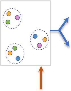
ARTICLE                                                                               NATURE COMMUNICATIONS | https://doi.org/10.1038/s41467-020-14974-x

aligned to human genome reference hg19 using Bismark (version 0.16.1)37. The               9.    Flavahan, W. A. et al. Insulator dysfunction and oncogene activation in IDH
aligned reads were then deduplicated, and the methylation call at each CpG site                  mutant gliomas. Nature 529, 110–114 (2016).
was determined by running the appropriate Bismark scripts. DNA methylation                 10.   Ke, Y. et al. 3D chromatin structures of mature gametes and structural
patterns were calculated using methclone38; epipolymorphism39 and PDR21 were                     reprogramming during mammalian embryogenesis. Cell 170, 367–381 e320
calculated using epihet (https://www.bioconductor.org/packages/devel/bioc/html/                  (2017).
epihet.html).                                                                              11.   Robson, M. I. et al. Constrained release of lamina-associated enhancers and
                                                                                                 genes from the nuclear envelope during T-cell activation facilitates their
ATAC-seq data processing. We used HMCan40 to obtain signal tracks from the                       association in chromosome compartments. Genome Res. 27, 1126–1138
alignment data.                                                                                  (2017).
                                                                                           12.   Nemeth, A. et al. Initial genomics of the human nucleolus. PLoS Genet. 6,
                                                                                                 e1000889 (2010).
Enhancer and super-enhancers enrichment. We calculated enhancer and super-
                                                                                           13.   Rousseeuw, P. J. Silhouettes: a graphical aid to the interpretation and
enhancer enrichment as the ratio between the expected value of observing a super-
                                                                                                 validation of cluster analysis. J. Comput. Appl. Math. 20, 53–65 (1987).
enhancer (or enhancer) per compartment and the expected value of observing a
                                                                                           14.   Ou, M., Cui, P., Pei, J., Zhang, Z. & Zhu, W. Asymmetric transitivity preserving
super enhancer (or enhancer) genome-wide.
                                                                                                 graph embedding. In: Proceedings of the 22nd ACM SIGKDD International
                                                                                                 Conference on Knowledge Discovery and Data Mining. (ACM, 2016).
Reporting summary. Further information on research design is available in                  15.   Perozzi, B., Al-Rfou, R. & Skiena, S. Deepwalk: online learning of social
the Nature Research Reporting Summary linked to this article.                                    representations. In: Proceedings of the 20th ACM SIGKDD international
                                                                                                 conference on Knowledge discovery and data mining. (ACM, 2014).
Data availability                                                                          16.   Fullwood, M. J. et al. An oestrogen-receptor-alpha-bound human chromatin
We obtained processed (.hic) formatted Hi-C data for both GM12878 and K562 cell-lines            interactome. Nature 462, 58–64 (2009).
from5 with GEO entry GSE63525. GM12878 ChIA-PET data accession code of 4D                  17.   Tang, Z. et al. CTCF-mediated human 3D genome architecture reveals
Nucleome consortium (https://commonfund.nih.gov/4dnucleome) is 4DNES7IB5LY9
                                                                                                 chromatin topology for transcription. Cell 163, 1611–1627 (2015).
(CTCF) and 4DNESZ25MOZV (RNAPII). We obtained raw ChIA-PET for CTCF and
                                                                                           18.   Hnisz, D., Shrinivas, K., Young, R. A., Chakraborty, A. K. & Sharp, P. A. A
RNAPII factor for K562 cell-line from ENCODE. We processed raw files to produce                   phase separation model for transcriptional control. Cell 169, 13–23 (2017).
loops follow the Links: https://www.encodeproject.org/experiments/ENCSR000BZY/ and         19.   Core, L. J. et al. Analysis of nascent RNA identifies a unified architecture of
https://www.encodeproject.org/experiments/ENCSR000CAC/. We used ATAC-seq data
                                                                                                 initiation regions at mammalian promoters and enhancers. Nat. Genet. 46,
generated by41 GEO entry GSE47753. We downloaded signal bigwig tracks for DHS and
                                                                                                 1311–1320 (2014).
histone modifications from the ENCODE consortium using the following link: http://ftp.      20.   Setty, M. et al. Inferring transcriptional and microRNA-mediated regulatory
ebi.ac.uk/pub/databases/ensembl/encode/integration_data_jan2011/byDataType/signal/               programs in glioblastoma. Mol. Syst. Biol. 8, 605 (2012).
jan2011/bigwig/. We downloaded super-enhancer annotations for GM12878 dbSuper
                                                                                           21.   Landau, D. A. et al. Locally disordered methylation forms the basis of
database42 (https://asntech.org/dbsuper/). We obtained enhancer data for GM12878
                                                                                                 intratumor methylome variation in chronic lymphocytic leukemia. Cancer Cell
from DENdb enhancers database43 (https://www.cbrc.kaust.edu.sa/dendb/), and used                 26, 813–825 (2014).
only high quality enhancers with a minimum score of 3 as assessed by DHS signal. We        22.   Roadmap Epigenomics, C. et al. Integrative analysis of 111 reference human
downloaded RNA-seq quantified gene expression files from ENCODE with the following
                                                                                                 epigenomes. Nature 518, 317–330 (2015).
GEO accessions: GSE88583, GSE88627, GSM958730, GSE90222, GSE78553, GSE78555.
                                                                                           23.   Gurukar, S. et al. Network Representation Learning: Consolidation and
We downloaded GRO-seq signal tracks described in ref. 19 from GEO accession number               Renewed Bearing. Preprint at arXiv:190500987 (2019).
GSE60456. For replication time data, we downloaded signal tracks from the ENCODE           24.   Zhang, D., Yin, J., Zhu, X., Zhang, C. Network representation learning: a
consortium using the following link: http://hgdownload.cse.ucsc.edu/goldenPath/hg19/             survey. IEEE Transactions on Big Data (2018).
encodeDCC/wgEncodeUwRepliSeq/. We obtained NAD enriched regions published in12
                                                                                           25.   Goyal, P. & Ferrara, E. Graph embedding techniques, applications, and
for hg18 reference. We used liftOver tool to map regions to hg19 reference. We only
                                                                                                 performance: a survey. Knowl.-Based Syst. 151, 78–94 (2018).
considered mapped regions with 0.95 confidence.                                             26.   Fotuhi Siahpirani, A., Ay, F. & Roy, S. A multi-task graph-clustering approach
                                                                                                 for chromosome conformation capture data sets identifies conserved modules
                                                                                                 of chromosomal interactions. Genome Biol. 17, 114 (2016).
Code availability                                                                          27.   Saramäki, J., Kivelä, M., Onnela, J.-P., Kaski, K. & Kertesz, J. Generalizations
SCI code is available on https://github.com/TheJacksonLaboratory/sci and https://github.         of the clustering coefficient to weighted complex networks. Phys. Rev. E 75,
com/TheJacksonLaboratory/sci-DNN.                                                                027105 (2007).
                                                                                           28.   Chen, T., Guestrin, C. Xgboost: a scalable tree boosting system. In: Proceedings
                                                                                                 of the 22nd ACM SIGKDD International Conference on Knowledge Discovery
Received: 5 December 2018; Accepted: 11 February 2020;                                           and Data Mining (ACM, 2016).
                                                                                           29.   Ho T. K. Random decision forests. In: Proceedings of 3rd International
                                                                                                 Conference on Document Analysis and Recognition. (IEEE, 1995).
                                                                                           30.   Consortium, E. P. An integrated encyclopedia of DNA elements in the human
                                                                                                 genome. Nature 489, 57–74 (2012).
                                                                                           31.   Weirauch, M. T. et al. Determination and inference of eukaryotic
References                                                                                       transcription factor sequence specificity. Cell 158, 1431–1443 (2014).
1.   Schmitt, A. D., Hu, M. & Ren, B. Genome-wide mapping and analysis of                  32.   Grant, C. E., Bailey, T. L. & Noble, W. S. FIMO: scanning for occurrences of a
     chromosome architecture. Nat. Rev. Mol. Cell Biol. 17, 743–755 (2016).                      given motif. Bioinformatics 27, 1017–1018 (2011).
2.   Lieberman-Aiden, E. et al. Comprehensive mapping of long-range interactions           33.   Pohl, A. & Beato, M. bwtool: a tool for bigWig files. Bioinformatics 30,
     reveals folding principles of the human genome. Science 326, 289–293 (2009).                1618–1619 (2014).
3.   Fortin, J. P. & Hansen, K. D. Reconstructing A/B compartments as revealed by          34.   Quinlan, A. R. & Hall, I. M. BEDTools: a flexible suite of utilities for
     Hi-C using long-range correlations in epigenetic data. Genome Biol. 16, 180                 comparing genomic features. Bioinformatics 26, 841–842 (2010).
     (2015).                                                                               35.   Harrow, J. et al. GENCODE: the reference human genome annotation for The
4.   Yaffe, E. & Tanay, A. Probabilistic modeling of Hi-C contact maps eliminates                ENCODE Project. Genome Res. 22, 1760–1774 (2012).
     systematic biases to characterize global chromosomal architecture. Nat. Genet.        36.   Kundaje, A. et al. Ubiquitous heterogeneity and asymmetry of the chromatin
     43, 1059–1065 (2011).                                                                       environment at regulatory elements. Genome Res. 22, 1735–1747 (2012).
5.   Rao, S. S. et al. A 3D map of the human genome at kilobase resolution reveals         37.   Krueger, F. & Andrews, S. R. Bismark: a flexible aligner and methylation caller
     principles of chromatin looping. Cell 159, 1665–1680 (2014).                                for Bisulfite-Seq applications. Bioinformatics 27, 1571–1572 (2011).
6.   Di Pierro, M., Cheng, R. R., Lieberman Aiden, E., Wolynes, P. G. & Onuchic, J.        38.   Li, S. et al. Dynamic evolution of clonal epialleles revealed by methclone.
     N. De novo prediction of human chromosome structures: Epigenetic marking                    Genome Biol. 15, 472 (2014).
     patterns encode genome architecture. Proc. Natl Acad. Sci. USA 114,                   39.   Landan, G. et al. Epigenetic polymorphism and the stochastic formation of
     12126–12131 (2017).                                                                         differentially methylated regions in normal and cancerous tissues. Nat. Genet.
7.   Chen, Y. et al. Mapping 3D genome organization relative to nuclear                          44, 1207–1214 (2012).
     compartments using TSA-Seq as a cytological ruler. J. Cell Biol. 217,                 40.   Ashoor, H. et al. HMCan: a method for detecting chromatin modifications
     4025–4048 (2018).                                                                           in cancer samples using ChIP-seq data. Bioinformatics 29, 2979–2986
8.   Tang, J. et al. LINE: Large-scale Information Network Embedding. In:                        (2013).
     Proceedings of the 24th International Conference on World Wide Web.                   41.   Buenrostro, J. D., Giresi, P. G., Zaba, L. C., Chang, H. Y. & Greenleaf, W. J.
     (International World Wide Web Conferences Steering Committee, 2015).                        Transposition of native chromatin for fast and sensitive epigenomic profiling

10                    NATURE COMMUNICATIONS | (2020)11:1173 | https://doi.org/10.1038/s41467-020-14974-x | www.nature.com/naturecommunications
You can also read