Performance of a Deep Neural Network at Detecting North Atlantic Right Whale Upcalls
←
→
Page content transcription
If your browser does not render page correctly, please read the page content below
This paper is part of a special issue on The Effects of
                                                                                                                 Noise on Aquatic Life

                                           Performance of a Deep Neural Network at
                                           Detecting North Atlantic Right Whale Upcalls
                                                    Oliver S. Kirsebom,1, a) Fabio Frazao,1 Yvan Simard,2, 3 Nathalie Roy,3 Stan Matwin,1, 4 and Samuel Giard3
                                                    1
                                                      Institute for Big Data Analytics, Dalhousie University, Halifax, Nova Scotia B3H 4R2, Canada
                                                    2
                                                      Fisheries and Oceans Canada Chair in underwater acoustics applied to ecosystem and marine mam-
                                                    mals, Marine Sciences Institute, University of Québec at Rimouski, Rimouski, Québec, Canada
                                                    3
                                                      Maurice Lamontagne Institute, Fisheries and Oceans Canada, Mont-Joli, Québec, Canada
                                                    4
                                                      Institute of Computer Sciences, Polish Academy of Sciences, Warsaw, Poland
                                                    (Dated: 3 March 2020)
arXiv:2001.09127v2 [eess.AS] 29 Feb 2020

                                                    Passive acoustics provides a powerful tool for monitoring the endangered North Atlantic right
                                                    whale (Eubalaena glacialis), but robust detection algorithms are needed to handle diverse and
                                                    variable acoustic conditions and differences in recording techniques and equipment. Here,
                                                    we investigate the potential of deep neural networks for addressing this need. ResNet, an
                                                    architecture commonly used for image recognition, is trained to recognize the time-frequency
                                                    representation of the characteristic North Atlantic right whale upcall. The network is trained
                                                    on several thousand examples recorded at various locations in the Gulf of St. Lawrence in
                                                    2018 and 2019, using different equipment and deployment techniques. Used as a detection
                                                    algorithm on fifty 30-minute recordings from the years 2015–2017 containing over one thou-
                                                    sand upcalls, the network achieves recalls up to 80%, while maintaining a precision of 90%.
                                                    Importantly, the performance of the network improves as more variance is introduced into the
                                                    training dataset, whereas the opposite trend is observed using a conventional linear discrim-
                                                    inant analysis approach. Our work demonstrates that deep neural networks can be trained
                                                    to identify North Atlantic right whale upcalls under diverse and variable conditions with a
                                                    performance that compares favorably to that of existing algorithms.
                                                     c 2020 Acoustical Society of America.       [http://dx.doi.org(DOI number)]

                                                    [XYZ]                                                                                        Pages: 1–12

                                           I. INTRODUCTION                                                       measures, which include vessel speed reduction and fish-
                                                                                                                 ing closure, were then put in place by the management
                                                The North Atlantic right whale (NARW, Eubalaena                  authorities in an effort to prevent the recurrence of such
                                           glacialis) comprises a small cetacean population that                 events (DFO, 2018).
                                           counted ∼ 400 individuals in 2017 (Hayes et al., 2018;                    The key information required to trigger vessel speed
                                           Pace et al., 2017; Pettis et al., 2019). Listed as endan-             reduction and fishing closure is the presence of the an-
                                           gered in Canada (COSEWIC, 2013), this population has                  imals in the highest risk areas. This information can
                                           been declining since 2010 (Pettis et al., 2019). NARW                 be acquired over large areas for short time windows
                                           used to be mainly distributed along the US continen-                  from systematic or opportunistic sightings from aircrafts
                                           tal shelf, up to the Bay of Fundy and the Western Sco-                or vessels. However, to obtain continuous round-the-
                                           tian shelf in Canada. This distribution, however, has                 clock information over the season, NARW detection with
                                           changed in the last decade (Davis et al., 2017). The oc-              passive acoustic monitoring (PAM) systems is needed
                                           casional yearly occurrence of a few individuals in the Gulf           (Simard et al., 2019). Various configurations of PAM
                                           of St. Lawrence in summer and fall markedly increased in              systems are possible for small- to large-scale coverages
                                           2015 and a high seasonal occurrence has continued since               (Gervaise et al., 2019b), including some supporting de-
                                           (Simard et al., 2019). This area is a site of intensive fixed-        tection in quasi real-time such as Viking-WOW buoys
                                           gear fishing. It is crossed by the main continental seaway            (https://ogsl.ca/viking/), Slocum gliders and fixed buoys
                                           that connects the Atlantic and the Great Lakes (Simard                (Baumgartner et al., 2019, 2013).
                                           et al., 2014). In 2017, 12 individuals died in the Gulf                   NARW upcall detection and classification (DC) algo-
                                           of St. Lawrence. The mortalities involved collisions with             rithms are a key component of such PAM systems. Sev-
                                           ships and entanglement in fixed fishing gear. Protection              eral algorithms, exploiting the time-frequency structure
                                                                                                                 of the call, have been used so far (Baumgartner et al.,
                                                                                                                 2011; Gillespie, 2004; Mellinger, 2004; Simard et al., 2019;
                                           a) Corresponding   author: oliver.kirsebom@dal.ca                     Urazghildiiev and Clark, 2006, 2007; Urazghildiiev et al.,

                                           J. Acoust. Soc. Am. / 3 March 2020      JASA/Performance of a Deep Neural Network at Detecting North Atlantic Right Whale Upcalls   1
2008). Their performance is dependent of the signal to spectrograms, which is also the strategy adopted in the
noise ratio (SNR), which varies with the range of the call- present work.
ing whale, the noise levels and the other biological and The paper is structured as follows. In Sec. II we
instrumentation factors (Gervaise et al., 2019b; Simard first describe how the acoustic data was collected, then
et al., 2019). The DC performance of these classical sig- discuss the generation of training datasets, the neural
nal processing methods under actual in situ recording network design and the training protocol. In Sec. III
conditions tends to plateau around a detection probabil- we present the results of the detection and classification
ity of about 50% (i.e. recall index) when the false detec- tasks, which are then discussed in Sec. IV. Finally, in
tion probability is kept below about 10% (DCLDE 2013; Sec. V we summarize and conclude.
Simard et al., 2019). The objective of the present study is
to test if modern machine-learning approaches can break
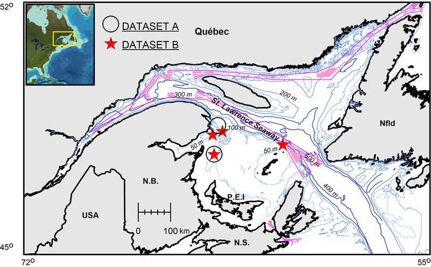
II. MATERIALS AND METHODS
this apparent DC performance ceiling.
Within the last decade, artificial neural networks A. Acoustic Data
have become the preferred machine-learning approach
for solving a wide range of tasks, outperforming exist- The PAM data were collected between 2015 and 2019
ing computational methods and achieving human-level at 6 stations in the southern Gulf of St. Lawrence (Fig. 1).
accuracy in domains such as image analysis (He et al., Two different deployment configurations were employed,
2015) and natural speech processing (Hinton et al., 2012). producing distinct datasets, A, B, and B∗ (Table I). In
Originally inspired by the human brain, neural networks addition to these datasets, we have also considered a
consist of a large number of interconnected “neurons”, third dataset, C, which is a subset of the DCLDE 2013
each typically performing a simple linear operation on dataset generated from PAM data collected in the Gulf
input data, specified by a set of weights and a bias, fol- of Maine in 2009.1
lowed by an activation function. In a supervised training In the case of dataset A, the PAM system was
approach, the network is given examples of labeled data, deployed from the surface, with the hydrophone
and the weights and biases are adjusted to produce the tethered to a real-time ocean observing Viking buoy
desired output using an optimization algorithm. Modern (Multi-Electronique Inc., Rimouski, Qc, Canada,
neural networks exhibit multi-layer architectures, which http://www.multi-electronique.com/buoy.html)
enable them to build complex concepts out of simpler with a 60-m long cable floating at the surface
concepts and hence learn a non-linear representation of for half of its length. The recording digital hy-
the data conducive to solving a given task. Therefore, drophone, at a depth of ∼ 30 m, was an ic-Listen
modern neural networks are often referred to as deep HF (Ocean Sonics, Truro Heights, N.S., Canada,
neural networks (DNNs), and the strategy of represent- https://oceansonics.com/product-types/iclisten-smart-
ing complex data as a nested hierarchy of concepts is hydrophones/). It sampled continuously the raw (0 gain)
referred to as deep learning. Two of the most commonly acoustic signal with 24-bit resolution. The receiving
encountered basic architectures are convolutional neural sensitivity of the hydrophone was −170 dB re 1 V µPa−1 .
networks (CNNs) and recurrent neural networks (RNNs), In the case of datasets B and B∗ , the PAM system
which are particularly well adapted to the tasks of ana- used short (< 10 m) “I”-type oceanographic moorings,
lyzing image data and sequential data, respectively. The with an anchor, an acoustic release, and streamlined
availability of large labeled datasets, containing millions underwater floats, for bottom deployment at depths
of labeled examples, has been a key factor in the success varying from 75 m to 125 m, with the autonomous
of DNNs in domains such as image analysis and natu- hydrophone ∼ 5 m above the seafloor. The recording
ral speech processing. Therefore, much of the current equipment consisted of AURAL M2 (Multi-Electronique
research in deep learning focuses on how to train DNNs Inc., Rimouski, Qc, Canada, http://www.multi-
more efficiently on smaller datasets. electronique.com/aural.html) sampling the 16-dB
Shallow neural networks have been employed for the pre-amplified acoustic signal with a 16-bit resolution
purpose of sound classification in marine bioacoustics at duty cycles of 15 min or 30 min every hour. The
since the 1990s, usually combined with a method of fea- receiving sensitivity of the HTI 96-MIN (High Tech Inc.,
ture extraction, e.g. (Bahoura and Simard, 2010), but Gulfport, MS) hydrophone equipping the AURAL is
also acting directly on the spectrogram (Halkias et al., −164±1 dB re 1 V µPa−1 over the < 0.5-kHz bandwidth
2013; Potter et al., 1994). In the last few years, the first used here. Further details can be found in (Simard
studies employing modern DNNs have been reported. et al., 2019).
Examples include classification of fish sounds (Malfante Because of the different acoustic equipment and de-
et al., 2018), detection and classification of orca vocal- ployment types, the recordings from the two datasets dif-
izations (Bergler et al., 2019), classification of multiple fered significantly in terms of signal amplitude and noise
whale species (McQuay et al., 2017; Thomas et al., 2019), background from different sources, including flow noise,
and detection and classification of sperm whale vocaliza- strum, and knocks resulting from the effects of tidal cur-
tions (Bermant et al., 2019). In all cases, CNNs have rents and the surface motion due to waves on the hy-
been leveraged to analyze the information encoded in drophone and deployment apparatus. Additional SNR
variability of the recordings is introduced by the differ-
2 J. Acoust. Soc. Am. / 3 March 2020 JASA/Performance of a Deep Neural Network at Detecting North Atlantic Right Whale UpcallsFIG. 1. (Color online) Map of the Gulf of St. Lawrence with bathymetry and seaways, showing the location of the PAM
stations. Circles indicate surface deployments (dataset A) while stars indicate bottom deployments (datasets B and B∗ ).
ent locations and depths at which the hydrophones were manually validated by an expert by examining the spec-
deployed in the southern Gulf of St. Lawrence, provid- trogram and labelled as “true” or “false” using the longer
ing different exposures to the above environmental condi- call pattern context in a ∼ 1-min window. In NARW call
tions and to the shipping noise field from the main seaway occurrence studies, the false detections are then elimi-
(Aulanier et al., 2016; Simard et al., 2019). The datasets nated. For the present work, however, both true and false
used here therefore represent a large range of conditions detections were extracted from the recordings and used
that can be encountered in realizing the DC task for the as “positives” and “negatives”, respectively, for building
low-frequency NARW upcall from acoustic data collected the training datasets A and B (Table II). For dataset C,
using different PAM systems. To develop a deep learning we have used the existing annotations from the DCLDE
model that is robust to such realistic range of variability, 2013 Challenge. Finally, we have built the composite
no effort was made to enhance the SNR before feeding datasets AB and ABC by combining all the samples from
the data to the neural network. the individual datasets.
To examine the accuracy of the validation protocol
B. Training and Test Datasets
used for producing datasets A and B, a second expert
was subsequently tasked with reviewing a subset of the
Datasets A and B were first analyzed with a clas- annotations. The review differed from the validation in
sical time-frequency based detector (TFBD) following several ways: the second expert had knowledge of both
(Mellinger, 2004) and (Mouy et al., 2009). This algo- the labels assigned by the first expert and the classifica-
rithm looks for a typical image of NARW upcall in the tion proposed by the DNN. The second expert used raw
SNR-enhanced (i.e., noise-subtracted), high-resolution spectrograms while the first expert used SNR-enhanced
(32 ms × 3.9 Hz) spectrogram of the recordings, and a spectrograms2 and a larger temporal context, including
detection is triggered by the degree of cross-coincidence. considerations of occurrence probability over the seasons.
The NARW upcall template used was a 1-s, 100–200 Hz Finally, the first expert was instructed to adopt a more
chirp with a ±10 Hz bandwidth. For further details, see conservative annotation strategy, always assigning a neg-
(Simard et al., 2019). The resulting detections were then ative label in cases of substantial doubt, whereas no such
J. Acoust. Soc. Am. / 3 March 2020 JASA/Performance of a Deep Neural Network at Detecting North Atlantic Right Whale Upcalls 3TABLE I. Datasets used in this work.
Dataset Deployment type Location Year(s) Analysis method
A Surface buoy Gulf of St. Lawrence 2019 Expert validation of detections reported by TFBD algorithm
B Bottom mooring Gulf of St. Lawrence 2018 Expert validation of detections reported by TFBD algorithm
∗
B Bottom mooring Gulf of St. Lawrence 2015–2017 Full manual analysis of fifty 30-min recordings
C Bottom mooring Gulf of Maine 2009 Full manual analysis of seven days of recordings
TABLE II. Number of samples in the datasets used for training and testing the classifiers. The composite datasets AB and
ABC were produced by combining all the samples from the individual datasets.
Training and validation Testing
Dataset
No. samples Positives Negatives No. samples Positives Negatives
A 1, 767 42% 58% 307 18% 82%
B 3, 309 61% 39% 579 59% 41%
C 3, 000 50% 50% − − −
AB 5, 076 55% 45% 886 45% 55%
ABC 8, 076 53% 47% − − −
instruction was given to the second expert. The results t0
of the annotation review will be discussed in Sec. IV.
Samples/day
200
(a)
The extracted segments are 3 s long and centered on train+val test
Dataset A
100 2019
the midpoint of the upcall, as determined by the TFBD
algorithm. However, the midpoint determined by the al- 0
gorithm rarely coincides with the actual midpoint of the t0
Samples/day
upcall, producing segments that are misaligned by up to 300
(b)
0.5 s in either direction. We note that such quasi-random 200 train+val test Positives
Dataset B
2018 Negatives
time shifts are desirable for training a DNN classifier be- 100
cause they encourage the network to learn a more general, 0
time translation invariant, representation of the upcall. 29 08 18 28 08 18 28 07 17 27
05- 06- 06- 06- 07- 07- 07- 08- 08- 08-
For the purpose of testing the classification perfor- time, t (month-day)
mance of the trained models, including their capacity for
generalizing, we split datasets A and B as follows: Sam-
ples obtained at times t < t0 were used for training and FIG. 2. (Color online) Time-split used to produce training
validation, while samples obtained at times t > t0 were and validation sets and test sets for Datasets A (a) and B (b).
retained for testing. Here, t0 was chosen to produce a
85:15 split ratio between the number of samples used for
training and validation and the number of samples used lap with the training datasets A and B, which originate
for testing (Fig. 2). This split implies temporal separa- from 2019 and 2018, respectively. Dataset B∗ was man-
tions of 52 min and 33 min between the latest sample in ually analyzed in its entire length by a third expert who
the training dataset and the earliest sample in the test identified 1, 157 NARW upcall occurrences.
dataset for A and B, respectively.
From the bottom deployments we also produced
dataset B∗ consisting of fifty 30-min segments from two C. Spectrogram and SNR Computation
years between 2015 and 2017 (Fig. 3). These data were First, the 3-s acoustic segments were downsampled to
used for testing the detection performance of the neural 1, 000 samples s−1 using MATLAB’s resample function,
network on continuous data. The data cover all seasons which employs a polyphase anti-aliasing filter. The spec-
and times of the day, hence providing a representative trogram representation was then computed on a dB scale
picture of the acoustic conditions found in the Gulf of using a window size of 0.256 s, a step size of 0.032 s (88%
St. Lawrence. Moreover, the data have no temporal over- overlap), and a Hamming window. These parameters
4 J. Acoust. Soc. Am. / 3 March 2020 JASA/Performance of a Deep Neural Network at Detecting North Atlantic Right Whale UpcallsA1796 (SNR=6.6)
B∗ B A
450
+0 dB
400
350 -20 dB
Frequency (Hz)
300
2015 2016 2017 2018 2019 -40 dB
Year 250
200
-60 dB
150
FIG. 3. (Color online) Temporal distribution of the training
datasets A and B and the continuous test dataset B∗ . 100 -80 dB
50
-100 dB
0
have been shown to be optimal for identifying NARW up- 0.0 0.5 1.0 1.5 2.0 2.5
calls (Gervaise et al., 2019a) and produce a spectrogram Time (s)
with (time, frequency) dimensions of 94 × 129. We note
that the spectrograms were fed to the network in their
FIG. 4. (Color online) Positive spectrogram sample from
raw form. In particular, no effort was made to normal-
dataset A. Superimposed is a 1-s window centered on the up-
ize the spectrograms to correct for systematic differences
in signal amplitude in the three datasets. This approach call (dashed line) and a trace drawn along the upcall (dotted
was adopted to produce the most general model possible. curve), as computed by the heuristic SNR algorithm described
For the estimation of the SNR value of each sample, in the text.
positive or negative, the following heuristic algorithm was
implemented: (1) A denoised spectrogram, Xd , was cre-
ated by subtracting first the median value of each time blocks with skip connections (He et al., 2016). CNNs
slice (to reduce broadband, impulsive noise) and then consist of a stack of convolutional layers followed by a few
subtracting the median value of each frequency slice (to fully connected layers. During the training process, the
reduce tonal noise). (2) The mid-point of the upcall was convolutional layers learn to extract patterns from the in-
determined by sliding a 1-s wide window across the de- put images, which are passed to the fully connected lay-
noised spectrogram while seeking to maximize, ers for classification (Goodfellow et al., 2016, Chapter 9).
The residual blocks in a ResNet are composed of convo-
sumt (maxf (Xd )) + sumf (maxt (Xd )) , lutional layers, but allow some connections between lay-
ers to be skipped, thereby avoiding “vanishing” and “ex-
in the frequency interval 80–200 Hz, where the subscripts ploding” gradients during training (He et al., 2016). We
indicate the axis (t:time, f :frequency) along which the used blocks with batch normalization (Ioffe and Szegedy,
mathematical operation is applied. (3) A trace was 2015) and rectified linear units (ReLU) (Nair and Hin-
drawn by connecting the pixels with the maximum value ton, 2010). The architecture was composed of eight such
in each time slice of Xd . (4) The median value of the blocks preceded by one convolutional layer and followed
original spectrogram, X, was computed along this trace, by a batch normalization layer, global average pooling
including also the three pixels immediately above and (Lin et al., 2013), and a fully connected layer with a soft-
below to account for the finite “width” of the upcall. max function, which is responsible for the classification.
(5) Finally, the median values of X in the 0.5-s adja- Finally, the output layer gives a score in the range 0–1
cent windows were computed for the frequency interval for each of the two classes (positive and negative), which
80–200 Hz and subtracted. Fig. 4 shows the result ob- add up to 1.
tained on a typical positive sample from dataset A. We
stress that SNR estimation is highly challenging for the E. Training Protocol
datasets considered in this work because of non-uniform
stationary noise, transient noise, and distortion of the We trained the network on two NVIDIA RTX 2080
upcalls due to propagation effects. Ti GPUs with 11GB of memory. Training was performed
with a batch size of 128 and terminated after a pre-set
number of epochs, N . That is, 128 samples were passed
D. Neural Network Architecture
through the network between successive optimizations of
The problem was set up as a binary classification the weights and biases, and every sample in the train-
task: A neural network was trained to classify the 3-s ing dataset was passed through the network N times.
spectrograms according to the criterion, contains (pos- Weights and biases were optimized with the ADAM op-
itive class, 1) or does not contain (negative class, 0) a timizer (Kingma and Ba, 2014) using the recommended
NARW upcall. We used a residual network (ResNet), parameters: an initial learning rate of 0.001, decay of
which is a CNN architecture mainly built of residual 0.01, β1 of 0.9, and β2 of 0.999. No effort was made to
J. Acoust. Soc. Am. / 3 March 2020 JASA/Performance of a Deep Neural Network at Detecting North Atlantic Right Whale Upcalls 5explore the effects of these parameters on the training For the computation of recall, precision, and false-
outcome. The network was trained to maximize the F1 positive rate, we merged adjacent positive (1) bins into
score, defined as the harmonic mean of precision and re- “detection events”, which extend from the lower edge
call, F1 = 2P R/(P + R), where R is the recall, i.e., the of the first bin, t, to the upper edge of the last bin,
fraction of the upcalls that were detected, and P is the t + N ∆t, N being the number of bins in the event. To
precision, i.e., the fraction of the detected upcalls that allow for minor temporal misalignments between anno-
were in fact upcalls. Thus, the F1 score considers both tations and detections, we adopted a temporal buffer
recall and precision and attaches equal importance to the of 1.0 s, effectively expanding every detection event to
two. [t − 2∆t, t + (N + 2)∆t]. Considering the primary in-
Initially, the network was trained using 5-fold cross- tended application of the detection algorithm, namely, to
validation with a 85:15 random split between the training quantify upcall occurrences in PAM data and provide oc-
and validation sets, allowing us to confirm that the op- currence times of sufficient accuracy to aid validation by
timization had converged without overfitting. Based on a human analyst, such a small temporal buffer is fully jus-
these initial training sessions, N = 100 was found to pro- tifiable. The recall was then computed as the fraction of
vide an optimal choice for all the training datasets. The annotated upcalls that exhibit at least 50% overlap with
network was then trained on the full training datasets a detection event, while the precision was computed as
without cross-validation for N = 100 epochs. This was the fraction of the detection events that exhibit at least
repeated nine times with different random number gener- 50% overlap with an annotated upcall. Any detection
ator seeds to assess the sensitivity of the training outcome event that did not overlap with an annotated upcall or
to the initial conditions. exhibited less than 50% overlap was counted as one false
positive for the computation of the false-positive rate.
F. Linear Discriminant Analysis
III. RESULTS
To establish a baseline against which to compare the
performance of the neural network, we implemented a A. Classification Performance
linear discriminant analysis (LDA) model following the
approach of (Martinez and Kak, 2001), noting that such The classification performance of the DNN and LDA
models have traditionally been adopted for solving sound classifiers on the test datasets are summarized in terms
detection and classification tasks in marine bioacoustics. of the average F1 score, recall, and precision obtained
First, the 94 × 129 spectrogram matrix was flattened to in the nine independent training sessions (Fig. 5). The
a vector of length 12, 126. Second, the dimensionality DNN model trained on the ABC dataset exhibits the best
was reduced by means of principal component analysis overall performance, achieving a recall of 87.5% and a
(PCA). Third, we trained the LDA classifier using a least- precision of 90.2% on the AB test set (with standard de-
squares solver combined with automatic shrinkage follow- viations of 1.1% and 1.2%) and outperforming the base-
ing the Ledoit-Wolf lemma (Ledoit and Wolf, 2004). The line LDA model by a statistically significant margin (as
training was repeated for several choices of PCA dimen- evident from Fig. 6 below).
sionality using a 85:15 random split between training and We have investigated the effect of increasing the size
validation sets, and the dimensionality yielding the best of dataset C by up to a factor of 10 (15, 000 upcalls), but
performance on the validation set was selected. found only a negligible improvement in the performance
of the DNN model. (We note that the DCLDE 2013
dataset contains 6, 916 logged calls. To produce a dataset
G. Detection Algorithm with 15, 000 upcalls we added time-shifted copies of the
For the purpose of detecting NARW upcalls in con- logged calls to the dataset.)
tinuous acoustic data, the following simple algorithm was We have also investigated the effect of discarding
implemented: First, the data were segmented using a samples with SNR below a certain minimum value,
window of 3 s and a step size of ∆t = 0.5 s. Each 3-s SNRmin , from the AB test set (Fig. 6). For the DNN
segment was then fed to the DNN classifier, producing a model, we observe a gradual increase in performance
sequence of classification scores between 0–1, which we as we restrict our attention to upcalls with increasingly
interpret as a time-series of upcall occurrence probabil- larger SNR values, with the recall improving from 89%
ities. Empirically, we found it useful to smoothen the at SNRmin ' 0 to 98% at SNRmin ' 12 and the precision
classification scores using a five-bin (2.5 s) wide averag- improving from 91% to 100% across the same range of
ing window. This greatly reduced the number of false SNR. The performance of the LDA model also improves
positives (factor of ∼ 5) at the cost of a modest increase with increasing SNR. This is especially true for the pre-
in the number of false negatives (factor of ∼ 2). Finally, cision, which improves from 70% at SNRmin ' 0 to 95%
we applied a uniform detection threshold, setting the bin at SNRmin ' 12, whereas the recall reaches a maximum
value to 1 (“positive”) when the score was greater than of 82% before worsening at the largest SNR values.
or equal to the threshold and 0 (“negative”) when it was In the following, we examine a small set of repre-
below. sentative spectrogram samples, which have been either
correctly classified or misclassified by the DNN model
6 J. Acoust. Soc. Am. / 3 March 2020 JASA/Performance of a Deep Neural Network at Detecting North Atlantic Right Whale Upcalls(a) DNN Performance (b) LDA Performance
90 90
43.3 10.4 16.8 66.4 64.4 64.7
A 41.2
62.0
9.2
60.0
13.7
65.4
A 58.2
77.7
65.5
63.7
64.5
65.2
80 80
48.0 88.3 83.7 46.5 79.7 73.4
B 40.3 89.4 82.4 B 75.0 89.7 87.6
80.0 88.1 86.7 70 33.9 71.8 63.1 70
Training dataset
Training dataset
69.1 87.8 85.0 60 60.0 76.6 74.6 60
AB 66.1
79.7
89.9
86.7
86.5
85.2
AB 55.4
65.6
83.2
71.0
79.3
70.5
50 50
80.5 90.1 88.8 60.6 71.9 70.5
ABC 71.3
93.0
90.1
90.2
87.5
90.2
ABC 55.2
67.4
74.9
69.1
72.1
68.9
40 40
A
B
AB
A
B
AB
Test dataset Test dataset
FIG. 5. (Color online) (a) DNN classification performance in terms of F1 score (top, large font), recall (middle, small font),
and precision (bottom, small font). Rows: training dataset; columns: test dataset. The colorscale indicates the F1 score. (b)
LDA classifier performance.
(Fig. 7). We divide the samples into true positives, true fiers on dataset B∗ , which has been subject to full manual
negatives, false positives, and false negatives, and for analysis.
each category we give three examples reflecting differ-
ent levels of certainty and difficulty as perceived by the B. Detection Performance on Continuous Data
second expert: (a) certain and easy, (b) certain, but dif-
ficult, and (c) uncertain. Here, it must be remembered The detection algorithm introduced in Sec. II G was
that the experts had access to a larger temporal context tested on dataset B∗ , which consists of fifty 30-minute
of ∼ 1 min to inform their decision. Notably, this may segments and has a total of 1, 157 upcalls. The number
have helped the expert to correctly identify calls with low of calls per file exhibits significant variation, ranging from
SNR in cases where the calls form part of a call series. none to 100 with a median value of 15.
A few observations can be made: the model is able to The performance of the detection algorithm is sum-
correctly identify upcalls with very different SNR (B2225, marized in terms of recall, precision, and false-positive
B3121); the model is able to correctly classify negatives rate (Fig. 8). The detection threshold is seen to pro-
containing potentially confusing patterns (A12), but not vide a convenient tunable parameter to adjust the detec-
always (A111); the model struggles in cases with low tion performance, depending on whether high precision
SNR (A134, A1858); the model can be confused by tonal or high recall is desired. One also notes that the nine
noises and multipath echoes (B205). These deficiencies independent training sessions produced detectors with
could potentially be resolved by enlarging the temporal very similar recall, but varying levels of precision. In
window, thereby giving the model access to the same particular, the best-performing detector achieves a recall
contextual information that is available to the human of 80%, while maintaining a precision above 90%, cor-
analyst, notably the appearance of an upcall series. responding to a false-positive rate of 5 occurences per
Finally, we highlight a limitation of the classification hour for this particular test dataset, while the “average”
results reported in this section. Since datasets A and detector achieves a recall of 60% for the same level of
B only contain samples flagged by the TFBD algorithm, precision.
the performance demonstrated on these datasets is not Finally, we have considered the effect of discard-
necessarily representative of the performance on a ran- ing samples with SNR below a certain minimum value,
dom selection of samples from a continuous recording, SNRmin , from the test dataset (Fig. 9). We observe
and the reported metrics (Fig. 5) cannot be readily ap- a gradual improvement in performance with increasing
plied to continuous data. In the next section, we address SNR. For example, by considering only samples with
this limitation by testing the performance of the classi- SNR > 4.0, the false-positive rate is reduced from 35
J. Acoust. Soc. Am. / 3 March 2020 JASA/Performance of a Deep Neural Network at Detecting North Atlantic Right Whale Upcalls 7On the other hand, we found that the DNN models
1.0
(a) generally performed poorly when trained on one dataset,
0.9 but tested on another (e.g. trained on A, but tested on B).
This behavior was not observed with the LDA models,
Recall
0.8
0.7 whose less performant solution appear to be less sensitive
to the training dataset.
0.6 The quality and accuracy of the training datasets
0.5 built as part of this work is limited by both the use of
a classical time-frequency based detector to select can-
1.0
(b) didate upcalls for expert validation and by human sub-
0.9 jectivity in the validation step. Any bias in the selec-
Precision
0.8 tion or validation step will be reflected in the training
0.7 dataset and hence affect the learning of the DNN. To ex-
DNN plore the bias in the validation step, a second expert was
0.6 LDA tasked with reviewing all the incorrectly classified seg-
0.5 ments (false positives as well as false negatives) and an
equally large number of correctly classified segments ran-
600
(c) Positives domly sampled from the AB test dataset (cf. Sec. II B).
Negatives
No. samples
The second expert flagged about half of the incorrectly
400 classified segments as “borderline”, implying that the
expert considered these classifications as being highly
200 uncertain. On the other hand, the second expert only
flagged 9% of the correctly classified segments as border-
0 line. Removing the borderline cases from the test data
−4 0 4 8 12 16 improves the recall and precision by 2% and 5%, respec-
SNRmin
tively. However, the second expert also changed some
of the labels not considered to be borderline. Adopt-
ing the second expert’s revised labels for the test data,
FIG. 6. (Color online) (a) Effect of discarding samples with the recall decreases by 6% while the precision increases
SNR < SNRmin from the AB test dataset on the recall of the by 2%. These changes in performance metrics testify to
DNN and LDA models trained on ABC. The lines show the the difficulty of obtaining accurate annotations on PAM
average recall obtained in the nine training sessions, while the data. It would be interesting to investigate the inter-
shaded bands show the 10% and 90% percentiles. (b) Same, annotator variability in a more systematic and controlled
for the precision. (c) Number of positive and negative samples manner than done here, but this is beyond the scope of
in the AB test dataset with SNR ≥ SNRmin . the present study. (For example, it can be argued that
the second expert may have been biased by prior knowl-
edge of the labels proposed by the first expert and the
to 6 occurences per hour, while maintaining a recall of DNN.)
90% and retaining more than 95% of the upcalls in the In order to obtain a realistic assessment of the perfor-
test dataset. mance that can be expected of the DNN model in a prac-
tical setting, we have tested the model’s ability to iden-
tify upcalls in continuous acoustic data representative of
IV. DISCUSSION the actual conditions required for a NARW upcall PAM
The DNN classifier has been found to outperform DC system. In order to obtain an unbiased estimate of
the baseline LDA model, achieving recall and precision the detection performance, these data were subject to a
of 87.5% and 90.2% on the AB test dataset. Addition- complete manual validation not resorting to the use of a
ally, the DNN models trained on the combined datasets classical detection algorithm to select candidate upcalls.
generally performed better than the models trained on The best-performing model achieved a recall of 80% while
the individual datasets, also when tested on the individ- maintaining a precision above 90%, corresponding to a
ual datasets. For example, models trained on AB con- false-positive rate of 5 occurences per hour for the cho-
sistently outperformed models trained exclusively on A, sen test dataset, while the “average” model only achieved
even when tested solely on A. In contrast, the baseline a recall of 60% for the same level of precision. However,
LDA model achieved worse performance when trained on by restricting our attention to upcalls with SNR & 4.0,
combined datasets. This is an important observation, be- the recall of the average model was increased to 85% for
cause it suggests that DNNs have the capacity to handle the same level of precision while retaining over 95% of
larger variance in the data, and indeed benefit from being the upcalls. Existing algorithms are capable of achieving
trained on data with greater variance, producing models similar levels of recall, but at the cost of a significantly
that are more robust to inter-dataset variability. higher false-positive rate (DCLDE 2013; Simard et al.,
2019).
8 J. Acoust. Soc. Am. / 3 March 2020 JASA/Performance of a Deep Neural Network at Detecting North Atlantic Right Whale UpcallsTrue Positives True Negatives False Positives False Negatives
B3121 (SNR=21.2) A1461 (SNR=2.4) A111 (SNR=-1.8) B205 (SNR=4.3)
450
400
350
Frequency (Hz)
300
a) 250
200
150
100
50
0
B2225 (SNR=5.9) A12 (SNR=11.8) A134 (SNR=4.5) A1858 (SNR=7.4)
450
400
350
Frequency (Hz)
300
b) 250
200
150
100
50
0
B1307 (SNR=7.5) B1484 (SNR=5.2) B1090 (SNR=3.9) B2582 (SNR=2.9)
450
400
350
Frequency (Hz)
300
c) 250
200
150
100
50
0
0.0 0.5 1.0 1.5 2.0 2.5 0.0 0.5 1.0 1.5 2.0 2.5 0.0 0.5 1.0 1.5 2.0 2.5 0.0 0.5 1.0 1.5 2.0 2.5
Time (s) Time (s) Time (s) Time (s)
FIG. 7. (Color online) Representative 3-s spectrogram samples. First column: true positives; second column: true negatives;
third column: false positives; fourth column: false negatives. For each category, three examples are given reflecting different
levels of certainty and difficulty as perceived by the second expert: (a) certain and easy; (b) certain, but difficult; (c) uncertain.
Spectrograms are labeled by their ID and SNR (in dB).
Finally, we note that a related work entitled “Deep siders acoustic data from several locations off the east
neural networks for automated detection of marine mam- coast of the US, whereas our work considers data from
mal species” (Shiu et al., 2020) has been published during the Gulf of St. Lawrence. Where (Shiu et al., 2020) pro-
the review of our paper. We would like to highlight the vides a comparison of several network architectures, our
complementary nature of the two studies. While similar work provides insights into the importance of dataset size
deployment techniques (surface buoys, bottom moorings) and variance. Moreover, our work provides insights into
and acoustic recorders were used, (Shiu et al., 2020) con- recall variability with SNR. Although a direct compar-
J. Acoust. Soc. Am. / 3 March 2020 JASA/Performance of a Deep Neural Network at Detecting North Atlantic Right Whale Upcalls 91.0 1.0
(a)
FPR (hour−1 )
0.8 0.8
101
Precision, P
Recall, R
0.6 0.6
0.4 0.4 100
R
0.2 0.2
P (a)
0.0 0.0 1.0
(b)
0.0 0.2 0.4 0.6 0.8 1.0
0.9
Detection threshold
Precision
0.0
0.8
50 1.0 2.0
0.7 4.0
40 0.8 8.0
FPR (hour−1 )
0.6
Precision, P
12.0
30 FPR-R 0.6 0.5
P-R 0.0 0.2 0.4 0.6 0.8 1.0
20 0.4 Recall
10 0.2
(b) 1500
0 0.0 (c)
0.0 0.2 0.4 0.6 0.8 1.0
Recall, R No. upcalls 1000
FIG. 8. (Color online) Detection performance on the contin- 500
uous test data (dataset B∗ ) in terms of recall (R), precision
(P), and false-positive rate (FPR). The lines show the aver-
age performance while the shaded bands show the 10% and 0
90% percentiles. (a) R and P versus the adopted detection −4 0 4 8 12 16 20
threshold. (b) P-R and FPR-R curves. SNRmin
FIG. 9. (Color online) Detection performance of the “aver-
ison of the detection performances achieved in the two
age” model on the continuous test data (dataset B∗ ) for the
studies cannot be made since different test datasets were
used, we note that the recall obtained by (Shiu et al., upcalls meeting the criterion SNR > SNRmin . The perfor-
2020) on continuous test data is somewhat higher than mance is shown in terms of recall (R), precision (P), and false-
the recall obtained in our study (95% vs. 87% for a false- positive rate (FPR) for the five cut-off values SNRmin = 0.0,
positive rate of 20 h−1 ). However, the difference is within 2.0, 4.0, 8.0, 12.0. (a) FPR vs. R; (b) P vs. R; (c) Number of
the range of variability that could be explained by differ- upcalls vs. SNRmin .
ences in SNR in the test data.
V. CONCLUSION could be achieved by further expanding the variance of
the training dataset. Using the DNN classifier, we im-
In summary, we have demonstrated that DNNs can plemented a simple detection algorithm, which exhib-
be trained to recognize NARW upcalls in acoustic record- ited good performance on continuous test data, achiev-
ings which have been made with different acoustic equip- ing a recall of 80% while maintaining a precision above
ment and deployment types, and hence differ significantly 90%. It would be interesting to explore still more so-
in terms of signal amplitude and noise background. By phisticated machine-learning approaches, most notably
training a DNN on a dataset comprised of about 4, 000 approaches that consider a wider temporal context, as
samples of NARW upcalls and an approximately equal done by the human experts, but this is beyond the scope
number of negative samples, we achieved recall and pre- of the present study and is left for future work. These
cision of 90% on a test dataset containing about 700 up- results highlight the potential of DNNs for solving sound
calls and a similar number of negatives. The DNN was detection and classification tasks in underwater acous-
observed to benefit from being trained on data with in- tics and motivate a community effort towards building
creased variance, suggesting that improved performance larger and improved training datasets, especially for de-
10 J. Acoust. Soc. Am. / 3 March 2020 JASA/Performance of a Deep Neural Network at Detecting North Atlantic Right Whale Upcallsployments with interfering noise events, which present Bergler, C., Schröter, H., Cheng, R. X., Barth, V., Weber, M.,
more challenging acoustic conditions. Nöth, E., Hofer, H., and Maier, A. (2019). “ORCA-SPOT: An
automatic killer whale sound detection toolkit using deep learn-
ing,” Sci. Rep. 9(1), 10997, doi: 10.1038/s41598-019-47335-w.
ACKNOWLEDGMENTS Bermant, P. C., Bronstein, M. M., Wood, R. J., Gero, S., and
Gruber, D. F. (2019). “Deep machine learning techniques for
We would like to thank C. Hilliard for proofread- the detection and classification of sperm whale bioacoustics,” Sci.
Rep. 9(1), 12588, doi: 10.1038/s41598-019-48909-4.
ing the manuscript. We are grateful to G. E. Davis, COSEWIC (2013). “COSEWIC assessment and status report on
H. Johnson, C. T. Taggart, C. Evers, and J. Theriault the North Atlantic right whale Eubalaena glacialis in Canada,”
for numerous discussions on NARW bioacoustics that Committee on the Status of Endangered Wildlife in Canada. Ot-
tawa, xi + 58 pp.
supported and guided the development of the neural- Davis, G. E., Baumgartner, M. F., Bonnell, J. M., Bell, J., Berchok,
network classifier. We thank Fisheries and Oceans C., Bort Thornton, J., Brault, S., Buchanan, G., Charif, R. A.,
Canada and the Natural Sciences and Engineering Re- Cholewiak, D., Clark, C. W., Corkeron, P., Delarue, J., Dudzin-
search Council, Discovery Grant to YS, for the collec- ski, K., Hatch, L., Hildebrand, J., Hodge, L., Klinck, H., Kraus,
S., Martin, B., Mellinger, D. K., Moors-Murphy, H., Nieukirk, S.,
tion and preparation of the datasets. The NARW detec- Nowacek, D. P., Parks, S., Read, A. J., Rice, A. N., Risch, D.,
tion algorithm is a contribution of the Canadian Foun- Širović, A., Soldevilla, M., Stafford, K., Stanistreet, J. E., Sum-
dation for Innovation MERIDIAN cyberinfrastructure mers, E., Todd, S., Warde, A., , and Van Parijs, S. M. (2017).
“Long-term passive acoustic recordings track the changing distri-
(https://meridian.cs.dal.ca/). This work was pre- bution of North Atlantic right whales (Eubalaena glacialis) from
sented at the fifth International Meeting on The Effects 2004 to 2014,” Sci. Rep. 7, 13460.
of Noise on Aquatic Life held in Den Haag, July 2019. DCLDE 2013. Unpublished results, https://soi.st-
andrews.ac.uk/dclde2013/.
DFO (2018). “Science advice on timing of the mandatory slow-
down zone for shipping traffic in the Gulf of St. Lawrence to
protect the North Atlantic right whale,” DFO Can. Sci. Advis.
Sec. Sci. Resp. 2017/042, 16 p.
Gervaise, C., Simard, Y., Aulanier, F., and Roy, N. (2019a). “Op-
APPENDIX: SUPPLEMENTARY MATERIAL timal passive acoustics systems for real-time detection and lo-
calization of North Atlantic right whales in their feeding ground
off Gaspé in the Gulf of St. Lawrence,” Can. Tech. Rep. Fish.
Upon manuscript acceptance we will provide the Aquat. Sci. 3346, ix + 57 pp.
code necessary to reproduce the results presented in the Gervaise, C., Simard, Y., Aulanier, F., and Roy, N. (2019b). “Per-
paper including initialization and training of the neural formance study of passive acoustic systems for detecting North
network, prediction on test data, and computation of test Atlantic right whales in seaways: the Honguedo strait in the Gulf
of St. Lawrence,” Can. Tech. Rep. Fish. Aquat. Sci. 3346, ix +
metrics, along with all necessary training and test data. 53 pp.
We will also provide more spectrogram samples (includ- Gillespie, D. (2004). “Detection and classification of right whale
ing expert annotation, model output, and SNR) and a calls using an “edge” detector operating on a smoothed spectro-
gram,” Can. Acoust. 32, 39–47.
complete diagram of the neural network architecture. Goodfellow, I., Bengio, Y., and Courville, A. (2016). “Deep learn-
ing book,” MIT Press 521(7553), 800.
Halkias, X. C., Paris, S., and Glotin, H. (2013). “Classification of
1 https://soi.st-andrews.ac.uk/static/soi/dclde2013/documents/ mysticete sounds using machine learning techniques,” J. Acoust.
Soc. Am. 134(5), 3496–3505, doi: 10.1121/1.4821203.
WorkshopDataset2013.pdf Hayes, S. A., Josephson, E., Maze-Foley, K., Rosel, P., Byrd, B.,
2 SNR enhancement can have two effects: It may allow extracting Chavez-Rosales, S., Cole, T., Engleby, L., Garrison, L., Hatch, J.
signals deeply embedded in noise, which cannot be seen in the raw et al. (2018). “US Atlantic and Gulf of Mexico marine mammal
spectrograms, but it may also generate artifacts that are mimick- stock assessments - 2017 (second edition),” NOAA Tech. Memo.
ing real signals. NMFS NE-245.
He, K., Zhang, X., Ren, S., and Sun, J. (2015). “Delving deep
Aulanier, F., Simard, Y., Roy, N., Gervaise, C., and Bandet, M. into rectifiers: Surpassing human-level performance on ImageNet
(2016). “Spatio-temporal exposure of blue whale habitats to classification,” in 2015 IEEE International Conference on Com-
shipping noise in St. Lawrence system,” DFO Can. Sc. Advis. puter Vision (ICCV), pp. 1026–1034, doi: 10.1109/ICCV.2015.
Sec. Res. Doc. 2016/090, p. vi + 26 p. 123.
Bahoura, M., and Simard, Y. (2010). “Blue whale calls classifica- He, K., Zhang, X., Ren, S., and Sun, J. (2016). “Deep residual
tion using short-time fourier and wavelet packet transforms and learning for image recognition,” in Proceedings of the IEEE con-
artificial neural network,” Digit. Signal Process. 20(4), 1256– ference on computer vision and pattern recognition, pp. 770–778.
1263, doi: 10.1016/j.dsp.2009.10.024. Hinton, G., Deng, L., Yu, D., Dahl, G. E., Mohamed, A., Jaitly,
Baumgartner, M. F., , and Mussoline, S. E. (2011). “A generalized N., Senior, A., Vanhoucke, V., Nguyen, P., Sainath, T. N.,
baleen whale call detection and classification system,” J. Acoust. and Kingsbury, B. (2012). “Deep neural networks for acoustic
Soc. Am. 129, 2889–2902. modeling in speech recognition: The shared views of four re-
Baumgartner, M. F., Bonnell, J., Van Parijs, S. M., Corkeron, search groups,” IEEE Signal Process. Mag. 29(6), 82–97, doi:
P. J., Hotchkin, C., Ball, K., Pelletier, L.-P., Partan, J., Peters, 10.1109/MSP.2012.2205597.
D., Kemp, J., Pietro, J., Newhall, K., Stokes, A., Cole, T. V. N., Ioffe, S., and Szegedy, C. (2015). “Batch normalization: Acceler-
Quintana, E., , and Kraus, S. D. (2019). “Persistent near real- ating deep network training by reducing internal covariate shift,”
time passive acoustic monitoring for baleen whales from a moored arXiv preprint arXiv:1502.03167 .
buoy: System description and evaluation,” Meth. Ecol. Evol. 10, Kingma, D. P., and Ba, J. (2014). “Adam: A method for stochastic
1476–1489. optimization,” arXiv preprint arXiv:1412.6980 .
Baumgartner, M. F., Fratantoni, D. M., Hurst, T. P., Brown, Ledoit, O., and Wolf, M. (2004). “Honey, i shrunk the sample
M. W., Cole, T. V. N., Van Parijs, S. M., , and Johnson, M. covariance matrix,” J. Portf. Manag. 30(4), 110–119, doi: 10.
(2013). “Real-time reporting of baleen whale passive acoustic 3905/jpm.2004.110.
detections from ocean gliders,” J. Acoust. Soc. Am. 134, 1814–
1823.
J. Acoust. Soc. Am. / 3 March 2020 JASA/Performance of a Deep Neural Network at Detecting North Atlantic Right Whale Upcalls 11Lin, M., Chen, Q., and Yan, S. (2013). “Network in network,” Potter, J. R., Mellinger, D. K., and Clark, C. W. (1994). “Ma-
arXiv preprint arXiv:1312.4400 . rine mammal call discrimination using artificial neural networks,”
Malfante, M., Mohammed, O., Gervaise, C., Dalla Mura, M., and J. Acoust. Soc. Am. 96, 1255–1262, doi: https://doi.org/10.
Mars, J. I. (2018). “Use of deep features for the automatic clas- 1121/1.410274.
sification of fish sounds,” in OCEANS’18 MTS/IEEE, Kobe, Shiu, Y., Palmer, K. J., Roch, M. A., Fleishman, E., Liu, X.,
Japan. Nosal, E-M., Helble, T., Cholewiak, D., Gillespie, D., and Klinck,
Martinez, A. M., and Kak, A. C. (2001). “PCA versus LDA,” IEEE H., (2020). “Deep neural networks for automated detection of
T. Pattern Anal. 23(2), 228–233, doi: 10.1109/34.908974. marine mammal species,” Sci. Rep. 10, 607.
McQuay, C., Sattar, F., and Driessen, P. F. (2017). “Deep learn- Simard, Y., Roy, N., Giard, S., and Aulanier, F. (2019). “North
ing for hydrophone big data,” in 2017 IEEE Pacific Rim Con- Atlantic right whale shift to the Gulf of St. Lawrence in 2015 as
ference on Communications, Computers and Signal Processing monitored by long-term passive acoustics,” Endang. Sp. Res. 40,
(PACRIM), pp. 1–6, doi: 10.1109/PACRIM.2017.8121894. 271–284, doi: https://doi.org/10.3354/esr01005.
Mellinger, D. K. (2004). “A comparison of methods for detecting Simard, Y., Roy, N., Giard, S., and Yayla, M. (2014). “Cana-
right whale calls,” Can. Acoust. 32, 55–65. dian year-round shipping traffic atlas for 2013: Volume 1,
Mouy, X., Bahoura, M., and Simard, Y. (2009). “Automatic recog- East Coast marine waters,” Can. Tech. Rep. Fish. Aquat. Sci.
nition of fin and blue whale calls for real-time monitoring in the 3091(Vol.1)E, xviii + 327 pp.
St. Lawrence,” J. Acoust. Soc. Am. 126. Thomas, M., Martin, B., Kowarski, K., Gaudet, B., and Matwin,
Nair, V., and Hinton, G. E. (2010). “Rectified linear units improve S. (2019). “Marine mammal species classification using convo-
restricted boltzmann machines,” in Proceedings of the 27th inter- lutional neural networks and a novel acoustic representation,”
national conference on machine learning (ICML-10), pp. 807– arXiv preprint arXiv:1907.13188 .
814. Urazghildiiev, I. R., and Clark, C. W. (2006). “Acoustic detection
Pace, R. M., Corkeron, P. J., and Kraus, S. D. (2017). “Statespace of North Atlantic right whale contact calls using the generalized
markrecapture estimates reveal a recent decline in abundance of likelihood ratio test,” J. Acoust. Soc. Am. 120, 1956–1963.
North Atlantic right whales,” Ecol. Evol. 7, 8730–8741. Urazghildiiev, I. R., and Clark, C. W. (2007). “Acoustic detection
Pettis, H. M., Pace, R. M. I., and Hamilton, P. K. (2019). “North of North Atlantic right whale contact calls using spectrogram-
Atlantic right whale consortium 2019 annual report card,” Re- based statistics,” J. Acoust. Soc. Am. 122, 769–776.
port to the North Atlantic Right Whale Consortium, 19 pp. Urazghildiiev, I. R., Clark, C. W., and Krein, T. P. (2008). “Detec-
tion and recognition of North Atlantic right whale contact calls
in the presence of ambient noise,” Can. Acoust. 36, 111–117.
12 J. Acoust. Soc. Am. / 3 March 2020 JASA/Performance of a Deep Neural Network at Detecting North Atlantic Right Whale UpcallsYou can also read