Progress and Proposals: A Case Study of Monocular Depth Estimation
←
→
Page content transcription
If your browser does not render page correctly, please read the page content below
Progress and Proposals: A Case Study of Monocular
                Depth Estimation

               Khalil Sarwari
               Forrest Laine
               Claire Tomlin

               Electrical Engineering and Computer Sciences
               University of California, Berkeley

               Technical Report No. UCB/EECS-2021-32
               http://www2.eecs.berkeley.edu/Pubs/TechRpts/2021/EECS-2021-32.html

               May 5, 2021
Copyright © 2021, by the author(s).
                            All rights reserved.

Permission to make digital or hard copies of all or part of this work for
personal or classroom use is granted without fee provided that copies are
not made or distributed for profit or commercial advantage and that copies
bear this notice and the full citation on the first page. To copy otherwise, to
republish, to post on servers or to redistribute to lists, requires prior specific
permission.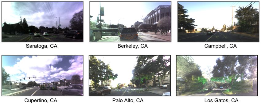
Progress and Proposals:
                 A Case Study of Monocular Depth Estimation

                                    by Khalil Sarwari

                                   Research Project

Submitted to the Department of Electrical Engineering and Computer Sciences,
University of California at Berkeley, in partial satisfaction of the requirements for the
degree of Master of Science, Plan II.

Approval for the Report and Comprehensive Examination:

                                        Committee:

                                  Professor Claire Tomlin
                                     Research Advisor

                                           (Date)

                                        *******

                                  Professor Sergey Levine
                                      Second Reader

                                         5/4/2021
                                           (Date)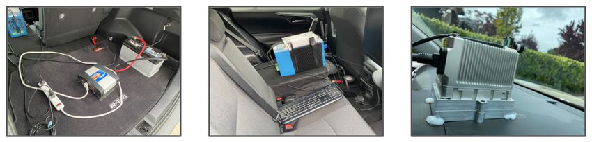
Acknowledgements

I would like to thank Professor Claire Tomlin for her support, advice and the opportunity to work
in the Hybrid Systems Lab. I am grateful to Shiry Ginosar and Tinghui Zhou for the introduction
to the world of research, and for all the early opportunities and guidance. I would like to thank
Somil Bansal and Varun Tolani for their invaluable mentorship and for teaching me a new level of
thoroughness, organization, and persistence. I would also like to thank Armin Askari and Amir
Zamir, who shared with me their experiences and helped me see the bigger picture. A special thank
you to Forrest Laine for his dedication, mentorship, and assistance with this project.
To my family and friends, who have given me inspiration, encouragement, and endless support
P ROGRESS AND P ROPOSALS :
A C ASE S TUDY OF M ONOCULAR D EPTH E STIMATION
 Khalil Sarwari, Forrest Laine, Claire Tomlin

 UC Berkeley
 {khalil.sarwari, forrest.laine, tomlin}@berkeley.edu

                                                 A BSTRACT

             Deep learning has achieved great results and made rapid progress over the past
             few years, particularly in the field of computer vision. Deep learning models are
             composed of artificial neural networks and a supervised, semi-supervised, or unsu-
             pervised learning scheme. Larger models have neural network architectures with
             more parameters, often resulting from more/wider layers. In this paper, we per-
             form a case study in the domain of monocular depth estimation and contribute both
             a new model as well as a new dataset. We propose PixelBins, a simplification to
             AdaBins, the existing state-of-the-art model, and obtain comparable performance
             to state-of-the-art methods. Our method achieves a ∼20× reduction in model size
             as well as an absolute relative error of 0.057 on the popular KITTI benchmark.
             Furthermore, we conceptualize and justify the need for truly open datasets. Con-
             sequently, we introduce a modern, extensible dataset consisting of high quality,
             cross-calibrated image+point cloud pairs across a diverse set of locations. The
             dataset is uniquely suited for the designation of truly open for a variety of rea-
             sons, such as a ∼100× reduction in cost to contribute a new image+pointcloud
             pair. We make our code and dataset publicly available1 and provide instructions
             for contributing to and replicating our experiments.

1       I NTRODUCTION

Modern deep learning systems can be decomposed into two main components: code and data. Model
architectures, training paradigms, and loss criterion fall under the former category. Data collection,
labeling, and preprocessing fall under the latter. Together, these components can produce spectacular
results on a wide variety of problems ranging from playing video games and detecting human poses
(Mnih et al. (2013), Wu et al. (2019)) to generating faces and text (Karras et al. (2020), Brown et al.
(2020)).
Pushing the boundaries by designing larger models and increasing dataset sizes, respectively, has
been closely tied to improved performance. On one hand, this implies current performance is limited
and falls short of its potential, since there always exists a larger model/dataset. On the other hand,
this association provides a sense of “closedness” to the problem at hand: rather than sources of
obstruction, these are two known channels for future performance gains (Levine (2021)).
In light of the centrality of code and data to the success of deep learning, we begin with a closer
look at their role, specifically in the domain of computer vision. After reviewing and assessing the
implications of these trends, we narrow our focus to the domain of monocular depth estimation.
The goal in monocular depth estimation is to estimate the depth of a scene from a single image; the
prediction result consists of a depth value for each pixel. Throughout our exploration, we employ
both a model-centric and data-centric perspective, and seek opportunities that reduce costs. In par-
ticular, we propose and evaluate both a new model as well as a new dataset for the monocular depth
estimation task.
The key contributions of this work are as follows:
    1
        https://github.com/khalilsarwari/depth

                                                     4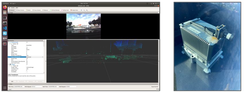
• A thorough analysis of models and datasets, two major components in deep learning, both
          in general and as related to monocular depth estimation
        • An efficient architecture for the monocular depth estimation task that is competitive with
          the state-of-the-art, yet exhibits a reduced model size and less overall complexity
        • A novel, truly open dataset for monocular depth estimation with benchmark results from
          our method. In order to initialize the dataset, we drive in 6 locations and collect im-
          age+point cloud pairs using a containerized codebase with a modern, cost-effective sensor
          suite

2     G ENERAL T RENDS
2.1    M ODELS A RE G ETTING L ARGER

      Figure 1: The trend in model size over the past five years. Note the log-scale on the y-axis.

Increasing the parameter count of a model enables it to fit a larger set of functions. This runs the
risk of overfitting, since, in an extreme scenario, a model with more parameters than data points
can simply “memorize” the dataset and fail to generalize. Deep learning models in particular seem
uniquely suited to excessive parameterization, and even more so with regularization techniques such
as Dropout (Srivastava et al. (2014)). Thus, model sizes have been able to grow rapidly. Figure
1 illustrates this trend on models applied to the popular ImageNet benchmark (Russakovsky et al.
(2015)).
A key breakthrough in the pursuit of larger models resulted from He et al. (2015), in which residual
connections were used to overcome issues with gradient flow. Allowing gradients to flow around and
through a layers increased the numerical stability of the backpropagation process for large networks.
This breakthrough resulted in the series of networks called ResNets, which are now used as the go-
to backbone of many modern models. Huang et al. (2016) took the residual connection idea to
an extreme by connecting each layer to every other layer in a feed-forward fashion. By explicitly
analyzing the various scalable dimensions, Tan & Le (2019) show that uniformly scaling the depth,
width, and resolution of a network is an effective way to obtain better performance. This produced a
line of architectures referred to as EfficientNets. Taking a learning-based approach, Real et al. (2018)
and Zoph et al. (2017) used evolutionary and reinforcement learning algorithms, respectively, to
tackle the problem of model architecture selection. Most recently, Dosovitskiy et al. (2020) applied
the transformer module, which was previously geared toward NLP, to vision tasks and delivered solid
results without the common dependency on convolutional layers. The proposed vision transformer
(ViT) is instead applied directly to sequences of image patches. Across all these changes, there has

                                                   5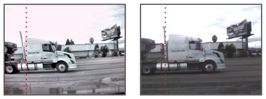
also been some reflection on what makes larger models perform better. For example, Frankle &
Carbin (2018) argue that not only are large models more expressive, but they have a higher chance
of being initialized correctly. In other words, the increased size of models could have more to do
with learning stability than raw expressive capacity.
Despite the tremendous progress attributed in part to increases in model sizes, this trend raises some
concerns. First and foremost, smaller, simpler models are inherently preferable, as they require
fewer resources during training/deployment, and are easier to interpret/understand. Furthermore,
there is an issue of democratization, as larger models require computer resources which may not be
accessible to the average individual. Not only does this exclude people from the performance gains,
but inaccessibility also creates issues regarding replication of results. Another increasingly impor-
tant concern is one of excessive energy consumption. These concerns have received attention and
potential solutions in the form of techniques such as model compression, quantization, and pruning.
While significant savings can be made on size, there is always some sacrifice in performance. Nev-
ertheless, these directions are still promising, and at the very least enable the deployment of these
models on smaller devices such as smartphones (Ignatov et al. (2018)).

2.2   DATASETS A RE G ETTING B IGGER

                          Name                 Author(s)             Size (K)
                         MNIST            LeCun et al. (2010)           60
                       CalTech 101        Fei-Fei et al. (2004)         12
                        CIFAR10            Krizhevsky (2009)            50
                          COCO              Lin et al. (2014)          330
                        ImageNet        Russakovsky et al. (2015)     1,200
                       Open Images      Kuznetsova et al. (2018)      9,000
                        JFT-300M            Sun et al. (2017)        300,000

                       Table 1: Sizes of various image recognition datasets.

In conjunction with growing model sizes, there has been an increase in dataset sizes as well, as
shown by Table 1. Among the reasons for this trend are declining costs in data storage and sensors
as well as increases in general online activity.
One of the earliest and most popular datasets is the MNIST dataset, introduced by LeCun et al.
(2010). The dataset consists of grayscale images of handwritten digits 0-9 (10 classes). The CI-
FAR10 dataset (Krizhevsky (2009)) on the other hand, consists of color images of 10 object cat-
egories such as airplanes and dogs. A key milestone in the scale of datasets was reached by the
ImageNet dataset (Russakovsky et al. (2015)). While the likes of MNIST and CIFAR10 are con-
sidered “toy” datasets in many respects, the ImageNet dataset is often considered a truer test of
real-world viability. Roughly two orders of magnitude larger than the popular ImageNet dataset, the
JFT-300M dataset (Sun et al. (2017)) is among the largest datasets used in an academic setting.
Like in the case of model sizes, there are concerns of accessibility and replication. It is worth
noting here that the JFT-300M dataset is not available to the public, whereas all the other datasets
in Table 1 are. While Sun et al. (2017) use the dataset to highlight the “Unreasonable Effectiveness
of Data in Deep Learning Era”, the community must simply take their word for it. If an attempt to
replicate such findings is made, it would most likely come from an organization or institution at a
similar scale, as opposed to the average individual. While the cost of compute reduces over time,
slowly mitigating the issue of model size, the concern of increased data requirements remains to be
addressed. We return to this issue and propose a solution in Section 3.2.1.

3     M ONOCULAR D EPTH E STIMATION

Given the vast variety of tasks and problems within deep learning, we select the task of monocular
depth estimation for a more specific analysis. The goal in monocular depth estimation is to infer
the depth corresponding to each pixel in a given image. This problem is fundamentally ill-posed,
since there are infinitely many real scenes that could produce a single given image. This makes

                                                  6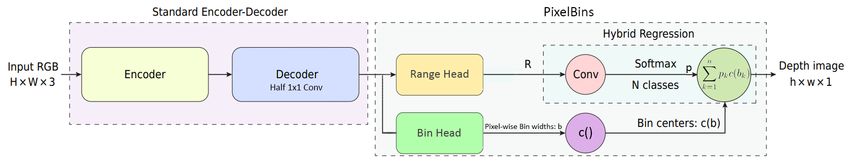
this task a monument to the allure of deep learning as a cure-all. With great expressive power and
data-intensive training, deep learning techniques utilize structural and spatial information as well as
priors to conjure up high-quality depth maps. A benefit of working on this task is that labels can be
collected very quickly using some type of depth sensor. As a result, the collected labels are consis-
tent, since they are provided automatically via machinery as opposed to being generated manually
by human labelers, where different labels may be selected for the same input due to differences in
interpretation.

3.1     M ODELS

Figure 2: The trend in monocular depth estimation model sizes over the past five years. Note the
log-scale on the y-axis. GFLOP metrics are omitted as they are not readily available for all models,
thus identical square markers are used.

The general trend of increasing model size also holds locally for the task of monocular depth es-
timation, as evidenced by Figure 2. The figure shows parameter count and performance changes
over time on the KITTI Eigen Split depth estimation benchmark (Geiger et al. (2013)). A popular
approach for this task is to use encoder-decoder networks (Godard et al. (2016), Casser et al. (2019),
Alhashim & Wonka (2018)). Later works have also taken from the recent popularity of transformer
modules (Ranftl et al. (2021), Bhat et al. (2020)).

3.1.1    C URRENT SOTA

The current state-of-the art monocular depth estimation method for the KITTI dataset benchmark
is called AdaBins developed by Bhat et al. (2020). Their architecture consists of two major com-
ponents: an encoder-decoder block and an adaptive depth-bin estimator block called AdaBins. The
AdaBins module uses a transformer to postprocess the output of the decoder block, and predict two
tensors. The first tensor consists of a range attention map, and the second consists of depth bins. Fu
et al. (2018) showed that predicting depth via classification as opposed to regression can lead to per-
formance gains. Thus, instead of predicting depth values directly, a linear combination of bin depths
and the range attention map is used for the final prediction, fusing regression with classification.
One key point is that the depth bins used in the linear combination for this method are shared for
all pixels in the image, and only the coefficients are predicted pixel-wise. These two predictions are
combined to get depth values for each pixel. Figure 3 reproduces the overview AdaBins architecture
from the paper for convenience.

                                                  7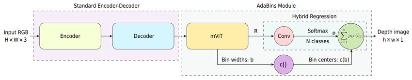
Figure 3: Overview of AdaBins architecture
3.1.2 P IXEL B INS
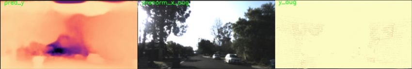
Figure 4: Qualitative Performance of PixelBins; please see Supplementary Materials for more qual-
itative visualizations on test set. Left: PixelBins depth map prediction. Middle: Ground truth
input image. Right: Ground truth point cloud. Note that the ground truth point cloud is sparse; the
fine-detail is best viewed by zooming in on an electronic copy.
Mindful of the concerns stemming from increased model size raised at the end of Section 2.1, we
break the trend of recent methods that use increasingly large and complex model architectures. The
intuition behind the powerful, yet expensive, transformer in Adabins was to aggregate global infor-
mation by processing the sequence that resulted from collapsing the spatial dimensions of the final
features. However, we found that the existing bottlenecking nature of the encoder can also provide
global information, and our experiments support that such a transformer module is not particularly
necessary. Thus, we replace the mViT with two heads consisting of a single 1x1 convolutional layer
which directly output the range attention map and pixel-wise bins as opposed to image-wise bins.
This increases the expressiveness of the model while significantly reducing parameter count. The
mViT is 5.8 millon parameters, while the two replacement heads from our method add up to roughly
32 thousand parameters. We replace half of the upsampling layers in the decoder with 1x1 con-
volutions as opposed to 3x3 convolutions due to computational constraints, and drop the proposed
chamfer loss from the paper for increased simplicity. Together, these changes result in the PixelBins
method shown in Figure 5. This method achieves comparable performance at a much lower cost
(both in terms of parameters and complexity) as illustrated by Table 2. Qualitative performance is
shown in Figure 4.
Figure 5: Overview of PixelBins architecture
3.1.3 I MPLEMENTATION D ETAILS
We implement our method in PyTorch (Paszke et al. (2017)). For training, we use the AdamW
optimizer with a weight-decay of 0.01. By leveraging automatic mixed precision training, we are
able to use a batch size of 16 across all experiments. We use the 1-cycle policy for the learning rate
with a max learning rate of 0.0002 and cosine annealing. For all results presented in Table 2, we
8train for 25 epochs following Bhat et al. (2020). For the results in Table 6 in the Supplementary
Materials, we train for 5 epochs per subset.
Method REL↓ Sq Rel↓ RMS↓ RMS log↓ Params (M)↓
DORN Fu et al. (2018) 0.072 0.307 2.727 0.120 110
VNL Yin et al. (2019) 0.072 - 3.258 0.117 44
BTS Lee et al. (2020) 0.059 0.245 2.756 0.096 47
AdaBins Bhat et al. (2020) 0.058 0.190 2.360 0.088 78
DPT-Hybrid Ranftl et al. (2021) 0.062 - 2.573 0.092 123
AdaBins Replication 0.057 0.214 2.594 0.087 78
PixelBins (Ours) 0.057 0.216 2.589 0.086 61
Table 2: Comparison of metrics on KITTI dataset. The numbers for the methods in the first group
are those reported from the corresponding original papers. We use the metrics defined in Bhat et al.
(2020); definitions are reproduced in the Supplementary Materials, along with a full comparison
with more metrics. The rightmost column lists the number of parameters (M=millions) in each
model. Best results are in bold, second best are underlined.
3.2 DATASETS
Name Author(s) Size (K) Camera Cost ($/unit) LiDAR Cost ($/unit)
KITTI Geiger et al. (2013) 26 350 75000
Waymo Sun et al. (2020) 12000 Unknown 75000
TODD Ours 222 229 800
Table 3: Quantitative comparison of various AV depth estimation datasets.
Why is it that the KITTI dataset is the standard dataset for this task? There are a couple of reasons.
To begin with, the KITTI dataset was the first dataset of its kind, so for the purpose of fair compari-
son, it makes sense to benchmark methods against what was used before. Second, the equipment and
resources needed to collect a dataset are not always readily available, and LiDAR equiment in partic-
ular has been relatively costly in the past. That being said, there have been other AV depth datasets
released since. Since each new dataset corresponds to an independent organization, attention often
shifts from one to the next and there is a lack of an adaptive and accessible standard.
3.2.1 T RULY O PEN DATASETS
Figure 6: The difference between traditional open datasets (left) and truly open datasets (right). Left:
Traditional open datasets, where data is made available for download, and the data source is “read-
only”. Right: Truly open datasets, where the broader community is not only able to train/evaluate
their own models, but also contribute to the diversity of the dataset. Instructions on how to contribute
new datapoints is provided, and the dataset is designed to expand in an organized and systematic
fashion.
To this end, we introduce the notion of a truly open dataset. Figure 6 captures the core of this notion
via a comparison to traditional datasets. Despite the majority of the work setting up a deep learning
pipeline involving data preparation, there seems to be a disproportionate focus on code (Ng (2021)).
9Indeed, data collection is a difficult process so most practicioners would rather focus on building
models/architectures. See Section 5.2.4 in the supplementary materials for examples of the obstacles
that are encountered. Obstacles such as these give all the more reason to have truly open datasets. By
distributing the burden of dataset curation, datasets can be scaled with regards to both quantity and
quality, while addressing concerns of accessibility raised at the end of Section 2.2. Contributions
to dataset can be driven by error analysis across community-wide deployments, leading to not only
more data, but higher quality data (Ng (2021)).
From a theoretical standpoint, deep learning models generally have low bias for moderately sized
datasets. These models have many parameters and, in the limit, are able to approximate any function
(Pinkus (1999)); they can easily overfit on small sized datasets. A large portion of error then can
be attributed to problems of variance. Constructing large, high quality datasets addresses this issue
directly, further supporting the utility of truly open datasets.
The benefits of truly open datasets are summarized as follows:
• Scale: Distributing the data collection process over multiple sources mitigates many issues
associated with aggregating large amounts of data
• Quality: By not fixing the dataset and setting standards for contribution, the dataset can be
corrected over time, as well as augmented to address community-discovered edge cases
• Accessibility: The dataset is a product of the collective efforts of the community, and
enables scale/quality that would previously have been restricted to large organizations
and corporations. Furthermore, the process of contributing data is streamlined and well-
documented to facilitate a seamless contribution experience
3.2.2 T RULY O PEN D EPTH DATASET
Figure 7: Sample images from Berkeley subfolder of TODD dataset with LiDAR points overlaid.
We introduce the Truly Open Depth Dataset (TODD), as a truly open AV monocular depth estimation
dataset, the first dataset of its kind.
The dataset consists of 222,000 cross-calibrated image-depth map pairs across 6 physical locations at
the time of release. Each pair is named after the UTC timestamp at which it was taken, and is placed
in a folder corresponding to coarse geographical location (city). Both sensors capture at a rate of
10 hz, and the image-depth map pairs are synchronized using the ApproximateTimeSynchronizer in
ROS within an interval of 50 milliseconds. Each location consists of 37,000 pairs, roughly one hour
of collection per location. Images are captured at a resolution of 960x1280 and then cropped and
resized to a resolution of 352x704 to match the KITTI dataset. The Berkeley location is selected as
the test set due to its diversity in scenery and objects. A sample set of images is provided in Figure 7;
please refer to the Supplementary Materials for additional sample images and data collection details.
This dataset is uniquely suited for truly openness due to the following reasons. First, the sensor
suite is relatively low cost, as shown in Table 3. Second, the data collection procedure has been con-
tainerized using Docker2 , which helps address challenges involving computational reproducibility
Boettiger (2015). Thus, once the sensors are obtained, plugged into a Docker-compatible machine
and calibrated, there is no further configuration necessary to collect more data in a manner that is
consistent.
2
https://www.docker.com/
10Figure 8 highlights the relation between performance and more data on TODD. Indeed, this ex-
periment serves as a testament to the centrality of data to building intelligent systems, and further
justifies efforts to create and sustain truly open datasets.
ID Location
1 Campbell
2 Cupertino
3 Los Gatos
4 Palo Alto
5 Saratoga
Figure 8: Absolute relative error (REL) on Test Berkeley
TODD test set as size of training set increases.
See Table 6 for additional performance metrics. Table 4: TODD locations
Recently, Ng (2021) noted that the benefits of larger datasets might be overstated in an effort by
organizations to assert dominance over the field. The importance of high quality data, as opposed
to quantity, has been overlooked. Indeed, the relation of data quantity to performance may not be
one that is necessary for satisfactory performance, but our analysis does seem to indicate that sheer
quantity is often sufficient. Thus, the importance of having extensible, community driven datasets
still stands.
4 C ONCLUSION
There has been tremendous progress in deep learning over the past few years, with particularly
notable results in computer vision. Much of this progress is associated with increasing model sizes
or training on larger datasets. We begin by looking at the popular ImageNet benchmark and the
associated model size and performance over time. We also perform a comparison of computer
vision datasets, and observe a similar increasing trend.
We then narrow our focus on these factors to the task of monocular depth estimation. While the
trends speak for themselves, viewing increased model size as a channel for improvement runs the
risk of excess in parameters, among other concerns. We propose PixelBins, a simplified model,
that breaks the trend of increases in model sizes while maintaining competitive performance on the
popular KITTI benchmark.
Furthermore, we introduce the notion of truly open datasets in an effort to address concerns of data
accessibility while maintaining competitive quantity and quality of data. We contribute TODD,
a novel depth estimation dataset that uniquely suited for extensions. We document the collection
process in detail, and containerize it to further facilitate future contributions.
Overall, we believe that mindfulness of these code-centric and data-centric approaches can lead to
less excess in the design of models as well as increased accessibility.
11R EFERENCES
Ibraheem Alhashim and Peter Wonka. High quality monocular depth estimation via transfer learn-
ing. CoRR, abs/1812.11941, 2018. URL http://arxiv.org/abs/1812.11941.
Shariq Farooq Bhat, Ibraheem Alhashim, and Peter Wonka. AdaBins: Depth estimation using adap-
tive bins, 2020.
Carl Boettiger. An introduction to docker for reproducible research. ACM SIGOPS Operating
Systems Review, 49(1):71–79, Jan 2015. ISSN 0163-5980. doi: 10.1145/2723872.2723882. URL
http://dx.doi.org/10.1145/2723872.2723882.
Tom Brown, Benjamin Mann, Nick Ryder, Melanie Subbiah, Jared D Kaplan, Prafulla Dhari-
wal, Arvind Neelakantan, Pranav Shyam, Girish Sastry, Amanda Askell, Sandhini Agar-
wal, Ariel Herbert-Voss, Gretchen Krueger, Tom Henighan, Rewon Child, Aditya Ramesh,
Daniel Ziegler, Jeffrey Wu, Clemens Winter, Chris Hesse, Mark Chen, Eric Sigler, Ma-
teusz Litwin, Scott Gray, Benjamin Chess, Jack Clark, Christopher Berner, Sam McCan-
dlish, Alec Radford, Ilya Sutskever, and Dario Amodei. Language models are few-shot
learners. In H. Larochelle, M. Ranzato, R. Hadsell, M. F. Balcan, and H. Lin (eds.), Ad-
vances in Neural Information Processing Systems, volume 33, pp. 1877–1901. Curran Asso-
ciates, Inc., 2020. URL https://proceedings.neurips.cc/paper/2020/file/
1457c0d6bfcb4967418bfb8ac142f64a-Paper.pdf.
Vincent Casser, Soeren Pirk, Reza Mahjourian, and Anelia Angelova. Depth prediction without the
sensors: Leveraging structure for unsupervised learning from monocular videos. In Thirty-Third
AAAI Conference on Artificial Intelligence (AAAI-19), 2019.
Jiahe Cui, Jianwei Niu, Zhenchao Ouyang, Yunxiang He, and Dian Liu. ACSC: Automatic calibra-
tion for non-repetitive scanning solid-state lidar and camera systems, 2020.
Alexey Dosovitskiy, Lucas Beyer, Alexander Kolesnikov, Dirk Weissenborn, Xiaohua Zhai, Thomas
Unterthiner, Mostafa Dehghani, Matthias Minderer, Georg Heigold, Sylvain Gelly, Jakob Uszko-
reit, and Neil Houlsby. An image is worth 16x16 words: Transformers for image recognition at
scale, 2020.
Li Fei-Fei, Rob Fergus, and Pietro Perona. Learning generative visual models from few training
examples: An incremental bayesian approach tested on 101 object categories. Computer Vision
and Pattern Recognition Workshop, 2004.
Jonathan Frankle and Michael Carbin. The lottery ticket hypothesis: Training pruned neural net-
works. CoRR, abs/1803.03635, 2018. URL http://arxiv.org/abs/1803.03635.
Huan Fu, Mingming Gong, Chaohui Wang, Kayhan Batmanghelich, and Dacheng Tao. Deep Or-
dinal Regression Network for Monocular Depth Estimation. In IEEE Conference on Computer
Vision and Pattern Recognition (CVPR), 2018.
Andreas Geiger, Philip Lenz, Christoph Stiller, and Raquel Urtasun. Vision meets robotics: The
kitti dataset. International Journal of Robotics Research (IJRR), 2013.
Clément Godard, Oisin Mac Aodha, and Gabriel J. Brostow. Unsupervised monocular depth esti-
mation with left-right consistency. CoRR, abs/1609.03677, 2016. URL http://arxiv.org/
abs/1609.03677.
Kaiming He, Xiangyu Zhang, Shaoqing Ren, and Jian Sun. Deep residual learning for image recog-
nition. CoRR, abs/1512.03385, 2015. URL http://arxiv.org/abs/1512.03385.
Gao Huang, Zhuang Liu, and Kilian Q. Weinberger. Densely connected convolutional networks.
CoRR, abs/1608.06993, 2016. URL http://arxiv.org/abs/1608.06993.
Andrey Ignatov, Radu Timofte, William Chou, Ke Wang, Max Wu, Tim Hartley, and Luc Van Gool.
AI benchmark: Running deep neural networks on android smartphones. CoRR, abs/1810.01109,
2018. URL http://arxiv.org/abs/1810.01109.
12Tero Karras, Miika Aittala, Janne Hellsten, Samuli Laine, Jaakko Lehtinen, and Timo Aila. Training
generative adversarial networks with limited data. In Proc. NeurIPS, 2020.
Alex Krizhevsky. Learning multiple layers of features from tiny images. Technical report, 2009.
Alina Kuznetsova, Hassan Rom, Neil Alldrin, Jasper Uijlings, Ivan Krasin, Jordi Pont-Tuset, Shahab
Kamali, Stefan Popov, Matteo Malloci, Tom Duerig, and Vittorio Ferrari. The Open Images
Dataset V4: Unified image classification, object detection, and visual relationship detection at
scale. arXiv:1811.00982, 2018.
Yann LeCun, Corinna Cortes, and CJ Burges. Mnist handwritten digit database. ATT Labs [Online].
Available: http://yann.lecun.com/exdb/mnist, 2, 2010.
Jin Han Lee, Myung-Kyu Han, Dong Wook Ko, and Il Hong Suh. From big to small: Multi-scale
local planar guidance for monocular depth estimation, 2020.
Sergey Levine. What makes deep learning work?, 2021. URL https://www.youtube.com/
watch?v=s2B0c_o_rbw.
Tsung-Yi Lin, Michael Maire, Serge J. Belongie, Lubomir D. Bourdev, Ross B. Girshick, James
Hays, Pietro Perona, Deva Ramanan, Piotr Dollár, and C. Lawrence Zitnick. Microsoft COCO:
common objects in context. CoRR, abs/1405.0312, 2014. URL http://arxiv.org/abs/
1405.0312.
Volodymyr Mnih, Koray Kavukcuoglu, David Silver, Alex Graves, Ioannis Antonoglou, Daan
Wierstra, and Martin A. Riedmiller. Playing Atari with deep reinforcement learning. CoRR,
abs/1312.5602, 2013. URL http://arxiv.org/abs/1312.5602.
Andrew Ng. A chat with Andrew on mlops: From model-centric to data-centric AI, 2021. URL
https://www.youtube.com/watch?v=06-AZXmwHjo.
Adam Paszke, Sam Gross, Soumith Chintala, Gregory Chanan, Edward Yang, Zachary DeVito,
Zeming Lin, Alban Desmaison, Luca Antiga, and Adam Lerer. Automatic differentiation in
pytorch. 2017.
Allan Pinkus. Approximation theory of the mlp model in neural networks. Acta Numerica, 8:
143–195, 1999. doi: 10.1017/S0962492900002919.
René Ranftl, Alexey Bochkovskiy, and Vladlen Koltun. Vision transformers for dense prediction,
2021.
Esteban Real, Alok Aggarwal, Yanping Huang, and Quoc V. Le. Regularized evolution for image
classifier architecture search. CoRR, abs/1802.01548, 2018. URL http://arxiv.org/abs/
1802.01548.
Olga Russakovsky, Jia Deng, Hao Su, Jonathan Krause, Sanjeev Satheesh, Sean Ma, Zhiheng
Huang, Andrej Karpathy, Aditya Khosla, Michael Bernstein, Alexander C. Berg, and Li Fei-Fei.
ImageNet Large Scale Visual Recognition Challenge. International Journal of Computer Vision
(IJCV), 115(3):211–252, 2015. doi: 10.1007/s11263-015-0816-y.
Nitish Srivastava, Geoffrey Hinton, Alex Krizhevsky, Ilya Sutskever, and Ruslan Salakhutdinov.
Dropout: A simple way to prevent neural networks from overfitting. Journal of Machine
Learning Research, 15(56):1929–1958, 2014. URL http://jmlr.org/papers/v15/
srivastava14a.html.
Chen Sun, Abhinav Shrivastava, Saurabh Singh, and Abhinav Gupta. Revisiting unreasonable ef-
fectiveness of data in deep learning era. CoRR, abs/1707.02968, 2017. URL http://arxiv.
org/abs/1707.02968.
Pei Sun, Henrik Kretzschmar, Xerxes Dotiwalla, Aurelien Chouard, Vijaysai Patnaik, Paul Tsui,
James Guo, Yin Zhou, Yuning Chai, Benjamin Caine, et al. Scalability in perception for au-
tonomous driving: Waymo open dataset. In Proceedings of the IEEE/CVF Conference on Com-
puter Vision and Pattern Recognition, pp. 2446–2454, 2020.
13Mingxing Tan and Quoc V. Le. EfficientNet: Rethinking model scaling for convolutional neural
networks. CoRR, abs/1905.11946, 2019. URL http://arxiv.org/abs/1905.11946.
Yuxin Wu, Alexander Kirillov, Francisco Massa, Wan-Yen Lo, and Ross Girshick. Detectron2.
https://github.com/facebookresearch/detectron2, 2019.
Wei Yin, Yifan Liu, Chunhua Shen, and Youliang Yan. Enforcing geometric constraints of virtual
normal for depth prediction. In The IEEE International Conference on Computer Vision (ICCV),
2019.
Barret Zoph, Vijay Vasudevan, Jonathon Shlens, and Quoc V. Le. Learning transferable architectures
for scalable image recognition. CoRR, abs/1707.07012, 2017. URL http://arxiv.org/
abs/1707.07012.
145 S UPPLEMENTARY M ATERIALS
5.1 KITTI C OMPARISON D ETAILS
Method δ1 ↑ δ2 ↑ δ3 ↑ REL↓ Sq Rel↓ RMS↓ RMS log↓
DORN Fu et al. (2018) 0.932 0.984 0.994 0.072 0.307 2.727 0.120
VNL Yin et al. (2019) 0.938 0.990 0.998 0.072 - 3.258 0.117
BTS Lee et al. (2020) 0.956 0.993 0.998 0.059 0.245 2.756 0.096
AdaBins Bhat et al. (2020) 0.964 0.995 0.999 0.058 0.190 2.360 0.088
DPT-Hybrid Ranftl et al. (2021) 0.959 0.995 0.999 0.062 - 2.573 0.092
AdaBins Replication 0.966 0.996 0.999 0.057 0.214 2.594 0.087
PixelBins (Ours) 0.966 0.996 0.999 0.057 0.216 2.589 0.086
Table 5: Full comparison of performances on KITTI dataset on popular metrics. The numbers for
the methods in the first group are those reported from the corresponding original papers. We use the
metrics defined in Bhat et al. (2020), and measurements are made for the depth range from 0m to
80m. Best results are in bold, second best are underlined.
5.1.1 M ETRICS
Let yp be a pixel in depth image y, ŷp a pixel in the predicted depth image ŷ, and n the total number
of pixels for each depth image.
Pn kyp −ŷp k
Absolute relative error (REL): 1
qp P y
n
n
Root mean squared error (RMS): n1 p kyp − ŷp k2
y ŷ
Threshold accuracy (δi ): % of yp s.t. max( ŷpp , ypp ) = δ < thr for thr = 1.25, 1.252 , 1.253
Pn ky −ŷ k2
Squared Relative Difference (Sq. Rel): n1 p p y p
q P
n
RMSE log: n1 p k log yp − log ŷp k2
5.2 DATA C OLLECTION D ETAILS
Figure 9: Data collection hardware setup. Left: Power supply configuration. Middle: Computer
and monitor. Right: LiDAR and camera.
Figure 9 shows the hardware setup for the data collection procedure. An intermediate car battery was
used to supply enough current to satisfy our needs. A monitor was tied to the back of the passenger
side headrest for mobile development. The camera was fixed to the LiDAR using glue to prevent the
need to recalibrate, as shown in Figure 10. The camera+LiDAR was then mounted to a detachable
plate, so that the sensors could be moved in and out of the vehicle jointly.
15Figure 10: Data collection configuration. Left: RViz setup. Right: Close-up of LiDAR and camera.
5.2.1 C AMERA
We used the LI-USB30-M021C camera3 , an automotive global shutter color camera with a Sunex
DSL3774 wide-angle lens.
Figure 11: Rolling vs global shutter. Left: Image from traditional rolling shutter camera. Right:
Image from the global shutter camera used in TODD. The dotted red line represents the true vertical
axis.
Figure 11 highlights an advantage of a global shutter camera over a rolling shutter camera using
nearly identical sensors5 . The distortion issue faced by rolling shutter cameras is exacerbated with
orthogonal motion, proximity, and speeds. While satisfying all these conditions is rare, we consid-
ered this when selecting our sensor suite, and believe that it is a better choice in the pursuit of precise
and reliable perception.
5.2.2 L I DAR
For LiDAR we used the Livox Horizon LiDAR6 , a high-performance, low-cost LiDAR. The LiDAR
samples 120,000 points per second using a non-repetitive scanning pattern. At a 10 Hz snapshot
rate, the maximum number of returned points in a given label is 12,000 points. The non-repetitive
scanning pattern helps improve the quality of supervision. Instead of providing the same exact label
for consecutive captures, a different point cloud is returned even when objects are static. Another
notable observation here is that the LiDAR works accurately through the windshield of the car, and
could be cross-calibrated with the camera without any issues.
5.2.3 C ALIBRATION
Camera LiDAR cross calibration is generally an involved process, since points have to be located in
3D space rather than just 2D. This means the calibration target needs to appear suspended in space
3
https://www.leopardimaging.com/product/usb30-cameras/usb30-camera-modules/li-usb30-m021c/
4
http://www.optics-online.com/OOL/DSL/DSL377.PDF
5
The rolling shutter sensor uses the AR1032AT sensor, while the global shutter camera uses the AR1035AT
6
https://www.livoxtech.com/horizon
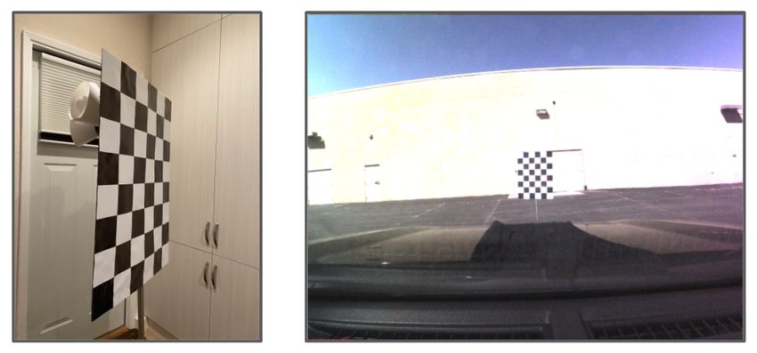
16Figure 12: Cross-Calibration procedure. Left: Close-up of chessboard. Right: Chessboard view
from mounted camera during calibration process.
with no obstacles in its near vicinity. We used the method entitled “Automatic extrinsic calibration
for non-repetitive scanning solid-state LiDAR and camera systems” from Cui et al. (2020), hereby
referred to as ACSC. The method aligns the 3D corner estimates with the 2D corners detected in
the image in an automated manner, and only requires the user to re-position the target in multiple
views. For more details on the method, as well as a detailed qualitative and quantitative analysis of
its performance, please refer to their paper.
We took 30 image/pointcloud pairs of the chessboard at various orientations and distances between
4m-8m, of which 3 pairs were unusable by the calibration method and automatically rejected. Figure
12 shows the chessboard and calibration setup.
5.2.4 E NCOUNTERED I SSUES
The data-collection portion of this report was very much subject to real-world problems and the
associated complexity, and thus resulted in a variety of obstacles. The following is a curated subset
of the issues we encountered, along with how we resolved them:
• Issue: When developing locally, the camera was working fine, but once we moved to the
car, the camera suddenly stopped working.
Resolution: After searching for software issues to no avail, we figured out that the longer
USB extension cable did not have enough bandwidth to supply the video frames fast
enough. By using a shorter USB cable, we were able to get the video working in the
car.
• Issue: The associated camera tool that allowed us to capture frames directly from the
camera was always emitting frames at half of the expected frame rate, making it hard to
sync the LiDAR and camera.
Resolution: It turns out that the camera tool was doing some image post-processing to
make the image look better, and in order to do so, it was halving the frame rate. By
removing this post-processing step, we were able to bring back the frame rate to what
was expected.
• Issue: We attempted to combine both the camera calibration and camera-LiDAR cross-
calibration into one process, but we kept getting the wrong intrinsic parameters.
Resolution: While we much preferred to be able to capture all the snapshots at once, it
turns out that the two calibration tasks are in some sense incompatible; the camera cali-
bration requires a much closer look at the chessboard, whereas the cross-calibration works
best at a distance. By splitting the process into two calibration stages, we collected the right
snapshots for each stage and were able to get the correct intrinsic and extrinsic parameters.
175.3 TODD D ETAILS
5.3.1 TODD L OCATIONS
Figure 13: TODD locations at time of first release, with LiDAR points projected onto image. The
data collected for each location respects the official city lines of that location.
5.3.2 TODD P ERFORMANCE C OMPARISON
IDs δ1 ↑ δ2 ↑ δ3 ↑ REL↓ Sq Rel↓ RMS↓ RMS log↓
1 0.698 0.9109 0.9719 0.1925 1.7762 8.1975 0.2551
1-2 0.7700 0.9411 0.9807 0.1682 1.5862 7.1841 0.2219
1-3 0.7876 0.9476 0.983 0.1569 1.4563 6.9824 0.2129
1-4 0.8104 0.954 0.9853 0.1498 1.3557 6.5571 0.2008
1-5 0.8243 0.9579 0.9858 0.1447 1.3657 6.4044 0.1947
Table 6: Performance on increasingly large subsets of TODD dataset.
185.3.3 Q UALITATIVE V ISUALIZATIONS
Figure 14: Qualitative Visualizations of PixelBins on TODD Test Set. White box selections mag-
nified for detail. Note that the ground truth point cloud is sparse; the fine-detail is best viewed by
zooming in on an electronic copy. Our method obtains best results on objects that are near; for
objects that are smaller, the boundaries are less clear.
19You can also read