Burrow emergence rhythms of Nephrops norvegicus by UWTV and surveying biases
←
→
Page content transcription
If your browser does not render page correctly, please read the page content below
www.nature.com/scientificreports
OPEN Burrow emergence rhythms
of Nephrops norvegicus by UWTV
and surveying biases
Jacopo Aguzzi1,2*, Nixon Bahamon1, Jennifer Doyle3, Colm Lordan3, Ian D. Tuck4,
Matteo Chiarini5,6, Michela Martinelli6 & Joan B. Company1
Underwater Television (UWTV) surveys provide fishery-independent stock size estimations of the
Norway lobster (Nephrops norvegicus), based directly on burrow counting using the survey assumption
of “one animal = one burrow”. However, stock size may be uncertain depending on true rates of burrow
occupation. For the first time, 3055 video transects carried out in several Functional Units (FUs)
around Ireland were used to investigate this uncertainty. This paper deals with the discrimination of
burrow emergence and door-keeping diel behaviour in Nephrops norvegicus, which is one of the most
commercially important fisheries in Europe. Comparisons of burrow densities with densities of visible
animals engaged in door-keeping (i.e. animals waiting at the tunnel entrance) behaviour and animals
in full emergence, were analysed at time windows of expected maximum population emergence.
Timing of maximum emergence was determined using wave-form analysis and GAM modelling. The
results showed an average level of 1 visible Nephrops individual per 10 burrow systems, depending
on sampling time and depth. This calls into question the current burrow occupancy assumption which
may not hold true in all FUs. This is discussed in relation to limitations of sampling methodologies and
new autonomous robotic technological solutions for monitoring.
The Norway lobster, Nephrops norvegicus (L.), is one of the most commercially important fisheries in Ireland
and also Europe1. The 2019 EU Total Allowable Catch (TAC) for Nephrops2 for the north east Atlantic Func-
tional Units (FU) was close to 44,000 tonnes, and valued at approximately 360 million EUR in 2 0163. Tradi-
tional fishery-dependent sampling methods such as commercial trawling provide indirect biomass estimates of
exploited stocks, by means of abundance indices derived from surface density data (i.e., the number of animals
per haul-swept a rea4–6).
However, animals construct and inhabit burrow systems used for shelter and for territorial c ontrol7 and are
not available for trawl capture when hiding in the s ubstrate8,9. The burrow emergence rhythmicity of popula-
tions causes marked fluctuations in catch rates over the 24-h10. Peaks in trawl Catch Per Unit Effort (CPUE)
shift in timing with increasing fishing depth11–13: from full night to dusk- dawn transitions, going from upper
to middle-lower shelves, to be finally fully diurnal (i.e. at midday) on upper and middle slopes. This indicates
that the species sets its timing of burrow emergence upon a maximum illumination threshold that varies on the
depth axis, based on the differential penetration of light as the sun progresses through its diurnal t rajectory10,14.
The diel rhythm of burrow emergence is more complex than previously thought and it can be subdivided in
three different phases11,15 : Full emergence, full retraction and an intermediate period in which individuals wait at
the burrow entrance (i.e. door-keeping16). To date, the proportion of animals not emerging from their burrows on
a daily basis is still largely undetermined, although acoustic tagging of individuals of a philetically closely related
species has offered some insight17. In addition to environmental light, other ecological reasons seem to modulate
the predisposition of individuals toward emergence or retraction. For example, crustaceans are at intermedi-
ate levels of the marine food webs and their feeding activity (coinciding with burrow emergence in the case of
Nephrops) is the product of a mortality risk ratio between hunger state and chances to meet visual predators18,19.
Alternative fishery-independent assessment methods as Underwater Television (UWTV) surveys using towed
camera-sledges, have been developed to estimate stock abundance20,21. Those video-based surveys are carried
out in several European countries and are coordinated through the International Council for the Exploitation
1
Instituto de Ciencias del Mar (ICM-CSIC), 08003 Barcelona, Spain. 2Stazione Zoologica of Naples (SZN),
80122 Naples, Italy. 3Marine Institute (MI), Oranmore, Galway H91 R673, Ireland. 4National Institute of
Water and Atmosphere (NIWA), Auckland 1010, New Zealand. 5Department of Biological, Geological and
Environmental Sciences, University of Bologna, 40126 Bologna, Italy. 6Institute of Marine Biological Resources and
Biotechnologies, National Research Council (CNR IRBIM), 60125 Ancona, Italy. *email: jaguzzi@icm.csic.es
Scientific Reports | (2021) 11:5797 | https://doi.org/10.1038/s41598-021-85240-3 1
Vol.:(0123456789)
www.nature.com/scientificreports/
of the Sea Working Group on Nephrops Surveys (WGNEPS)1,22,23. This more direct (i.e. image-based) method
of assessment counts burrow systems, based on their characteristic structural features (i.e. large crater-like
entrances4,24,25 and their characteristic arrangement individual burrow entrances20. Those systems are composed
of multiple entrances, shafts and tunnels and can be readily identified by classic features and orientation of the
individual burrow entrances, where the apexes of those entrances facing each other in a simple U-shaped system
or converging on one central point in a more developed system (i.e. T-shape)26,27. This method is independent
from the time of the day and season. The burrow system counts can be used as a relative or absolute index for
determination of Nephrops’ stock status and together with catch data can provide a Harvest Rate (HR; catch in
numbers/burrow numbers)28, 29.
To use UWTV burrow abundance to calculate catch and landings derived from an acceptable Harvest Rate
(HR = catch in numbers/UWTV abundance) it is necessary to adjust using agreed correction factor which takes
into account the bias associated with UWTV surveys. The key bias contributions for individual Nephrops Func-
tional Unit (FU) have been documented and the cumulative correction factor considers edge effect, burrow
identification, burrow detection and burrow o ccupancy28,29.
Given the strong territorial behavior of the species, burrow counting seems to be a good proxy for local popu-
lation abundance, assuming the condition “one burrow system, one animal”30, which is the current assumption for
Nephrops stock a ssessment28,29. The burrow system acts as the center of a strong territorial rhythmic behavior7,31,32
and two adult lobsters are rarely found in the same s helter33. No spatial segregation occurs between juveniles
and adults34 and the majority of juveniles build adult-juvenile burrow complexes, which become separated as
juveniles grow, and each individual develops its own s ection35. However, burrows systems could also be inhabited
by other benthic fish and crustacean species or may remain empty and intact for an unknown period of time after
the animals’ death (e.g. due to fishing or natural mortality30,36). These factors still pose uncertainties about the
true numbers of animals occupying video-counted burrow systems, representing a problem when using UWTV
data in stock assessment models30.
To improve knowledge of the stock assessment assumption “one burrow system, one animal” a precise tem-
poral description of burrow emergence rhythmicity could be provided by temporally distributed transects within
UWTV surveys, similar to that explored with trawl d ata11. The sum of animals engaged in both behaviours could
then be compared with counted burrows at phases of maximum population emergence. Unfortunately, temporally
scheduled UWTV operations have never been systematically performed and the analysis of rhythmic fluctuations
in video-observed animals performing full emergence and door-keeping is not yet available.
Here, we used UWTV survey data reporting densities of full emergence and door-keeping animals and bur-
row systems from more than three thousand video transects, conducted in the past decade around Ireland, to
temporally define both behaviours and their reciprocal relationship over the 24-h. Results on estimated densi-
ties of animals engaged in full emergence and door-keeping were then compared with burrow system density
estimates, to provide a comparison to the stock assessment assumption “1 burrow system, one animal”.
Materials and methods
The study areas and the UWTV surveys methodology. Video footage and derived data were col-
lected from 3055 UWTV transects conducted from 2002 to 2013 in FU areas in the seas around Ireland (Fig. 1).
Footage from each transect for all survey areas had a minimum recorded duration of 10 min. The counted
minutes of each transect was in line with the prevailing international counting procedure; in years 2002 to 2008
10 min were counted, and in years 2008 to 2013 7 min were counted28,29. For FU 16, 10 min were counted for all
years, due to the lower densities observed and the relative scale of variation between minutes was higher than
typically found in other areas. All considered data were collected in spring–summer surveys (from May to Sep-
tember) (Table 1), in order to avoid variations in the number of video-counted animals and based on reproduc-
tive and moulting cycles (see next section).
Sampling design followed either a randomised isometric grid with a station spacing dependent on the indi-
vidual survey area or a random stratified d esign37 (Table 1). The initial ground perimeter was established by
using a combination of integrated logbook-VMS38 and habitat data (see methods described in Ligas et al.39). The
final perimeter has been established using an adaptive approach where stations were located beyond the previ-
ously known perimeter of the ground, until the burrow system densities were zero or very close to zero. Once
established, the survey area was not changed between years.
At each station, the UWTV sledge was deployed and once stable on the seabed, a 10 min’ tow was recorded
onto DVD. The field of view of the camera (Kongsberg OE14-366) at the bottom of the screen with the sledge
flat on the seabed (i.e. no sinking), was validated at 75 cm by two parallel spot lasers. Vessel position (by Dif-
ferential Global Positioning System-DGPS) and sledge position (using an on-board Ultra Short Baseline-USBL,
transponder) were recorded every 2 to 5 s. USBL navigational data were used to calculate the video transect
distance over the ground, as required for surface density estimates (see next section). The navigational data were
quality controlled using an “R” script developed by the Marine I nstitute28,29.
Data processing. The same footage was viewed and counted by two scientists independently of each other
and burrows were identified based on key structural features from an established set of classification keys20,25,40.
All scientists were trained prior to counting following the ICES r ecommendations28,29, in such a way the counters
can be quite consistent in the recognition of a N. norvegicus burrow as compared to other species. Final burrow
densities were based on an average from the two independent counts after passing quality control processes
such as screening for outliers and use of Lin’s concordance CCC to evaluate counter performance20. The qual-
ity assured burrow density values were then corrected for stock specific survey cumulative bias as described in
ICES29.
Scientific Reports | (2021) 11:5797 | https://doi.org/10.1038/s41598-021-85240-3 2
Vol:.(1234567890)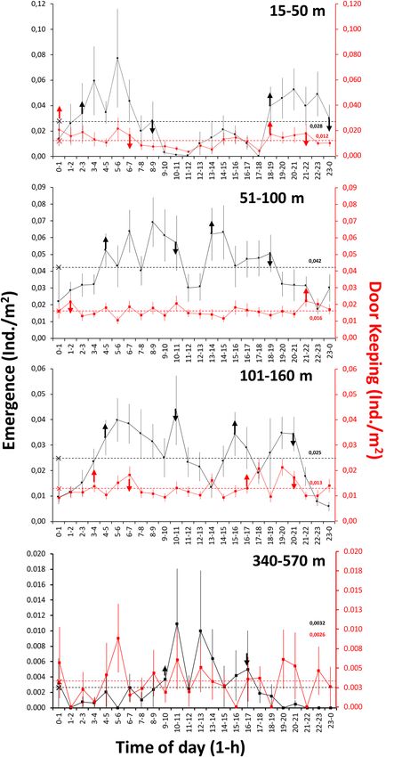
www.nature.com/scientificreports/
Figure 1. The UWTV survey areas around the Irish coast. Numbers represent the ICES Nephrops Functional
Units (FUs), as defined by the ICES Nephrops Working Group. Depth (m) for the study areas (GEBCO
bathymetry data). Map created using: R version 3.61 (2019–07-05) software, https://tinyurl.com/yy6rzlut.
Video-counts of door-keeping animals, defined as those with partial cephalothorax or claws were visible
across the burrow mouth entrance, and animals in full emergence which were entirely visible were available10,15.
As with burrow systems, densities of animals in door-keeping and full emergence were obtained for each transect
by dividing respective counts by the video-swept surface.
Each density estimate for burrow systems and animals in both behavioural categories was associated to a
time stamp, represented by the time at mid transect length. All density data were grouped per depth ranges
atterns11,41,42 nominally as:
within the upper and lower shelf, based on the previous knowledge from trawl catch p
15–50, 51–100, 101–160 and 340–570 m. No data were available for 161–339 m depth. Data for the bathymetric
range 340–570 m were only available in FU 16 for the years 2012 and 2013, and this inclusion was necessary
to characterize behavioural rhythms in the deepest range for comparison with shallow shelf observations (as
previously done with trawling11).
Scientific Reports | (2021) 11:5797 | https://doi.org/10.1038/s41598-021-85240-3 3
Vol.:(0123456789)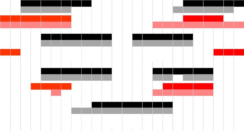
www.nature.com/scientificreports/
Depth range (m) Sampling grid spacing Sampling months
Number of
FU code Area Min Max (km) May Jun Jul Aug Sep UWTV transects
15 West Irish Sea 15 162 5.0 X X 1501
16 Porcupine Banks 343 570 6.0 X X X 115
17 Aran grounds, Galway Bay, Slyne Head 26 162 3.5 X X X X 854
19 South and SW coasts of Ireland 18 116 – X X X X 101
20–21 Labadie, Jones and Cockburn Banks 95 138 6.0 X X X 125
22 The Smalls 74 145 4.5 X X 635
Table 1. List of Nephrops functional units (FU), including their code number, area name and depth range.
FU grid spacing is shown for randomised isometric sampling designs. Random stratified sampling is used for
FU19. The distribution of UWTV surveys across summer months and number of transects in each FU is also
shown.
The rational for those depth groupings was that Nephrops burrow emergence is an adaptive life trait under
strong selection which can be temporally described as different on upper and lower shelves as well as s lopes11.
Moreover, the burrow emergence rhythm manifests itself similarly in all its geographic range, with coincident
nocturnal, crepuscular or diurnal timings according to the depth light driven peaks not blurred by the tidal
status10,43. This behaviour is constant through years, subjected only to a seasonal reproduction and growth
pattern (e.g. berried females do not e merge15,44,45), the effects of which were eliminated here by selecting only
summer data (see Table 1).
Statistical analysis. Firstly, we ran a waveform analysis to describe averaged full emergence and door-
keeping behavioural rhythms over the 24-h within the established depth ranges (see above). Waveforms plots
describe the phase of a rhythm as an averaged peak into a time series of density data for both behavioural cat-
egories. Waveform computing procedure was as follows46. A standard day was divided into 1-h intervals and
all density estimates for animals in full emergence and door-keeping were pooled together from all the surveys
within the same depth range and then averaged at corresponding 1-h timing.
The resulting set of averaged density estimates were then represented over the 24-h with their standard devia-
tions, plus the Midline Estimated Statistic of a Rhythm ( MESOR47). MESOR is a re-average of all waveform values
to be represented onto waveform plots as a horizontal threshold line. All waveform values above the threshold
delimit the duration of the peak (i.e. activity peak duration46). Waveforms for full emergence and door-keeping
density estimates were plotted together to highlight their temporal relationship.
Then, we fitted Generalised Additive Models (GAM) onto full emergence and door-keeping data for
spring–summer at the established depth ranges (see above), to achieve statistic formalization of observed emer-
gence patterns beyond data variability (Appendix 1). The package ‘mgcv’48 in R 49 was used with the restricted
maximum log-likelihood approach. The effects of the inter-annual variability and the variability among FUs
were assessed in the models. The Hour of the Day (HD), from zero to 23 h, was the covariate used to character-
ize behavioural rhythms. The day-length and the average location of the transects (latitude and longitude) were
adopted as spatiotemporal covariates in the full model, following the form:
E(NEP) = g −1 β0 + year + FU + s(HD, bs = cc, k = 24) + s Daylength + te(Lat, Lon) (1)
where E(NEP) is the Expected value of Nephrops full emergence or door-keeping, conditionally distributed
according to the Gamma distribution family. g is the log link function, β0 is the intercept. s is the smoothing
function with the term bs = "cc" specifying the 24 h’ knot based (k = 24) cyclic cubic regression spline. The day-
length was estimated as the difference between the sunrise and sunset times. te is the tensor smooth function
for the interaction among transect locations (i.e. latitude and longitude) accounting for spatial dependence on
diel activity rhythms affecting NEP. Alternatively to the te(Lat, Lon) effect, the potential effect of the station
locations per FU, te(Lat, Lon, by = FU), and the interaction between the station locations with the year survey
ti(Lat, Lon, year, d = c(2,1), were also tested in the models. The ti tensor product spline tested the significance
of the space-year interaction effect. The 2-dimensional space and the 1-dimensional year factor were specified
with the argument d = c(2,1).
The models showing significant HD term (i.e. behavioural rhythm), and other significant covariates substan-
tially improving the model variance were selected as the final models (see Appendix 1). The different models were
fitted and compared using the percentage of explained deviance and the Akaike Information Criterion (AIC)
to select the best one50. The range of AIC values of models within depth ranges was generally narrow and not
assumed to be critical for the final model choice. The selected final model followed the form (see Appendix 1):
E(NEP) = g −1 β0 + s(HD, bs = cc, k = 24) + f (Cov) (2)
where f(Cov) represented the term te(Lat, Lon) for the emergence and door keeping behaviours in the upper
depth range (15–50 m). In the case of the emergence behaviour at the depth ranges between 51 and 160 m and
door keeping at 101-160 m, f(Cov) represented the term s(Daylength). Because of the indistinguishable effect of
the terms te(Lat, Lon) or s(Daylength), on the NEP behavioural pattern (see Appendix 1), here we show results
and focus on the behaviour produced by the HD term of NEP.
Scientific Reports | (2021) 11:5797 | https://doi.org/10.1038/s41598-021-85240-3 4
Vol:.(1234567890)www.nature.com/scientificreports/
We averaged over periods of 1-h, and this probably resulted in models with relatively less variable behaviour
during the day, even if the general distribution of Nephrops in full emergence and door-keeping did not show
appreciable changes. The depth range models allowed identifying peaks timing and duration of full emergence
and door-keeping behaviours from the fitted values above the mean.
Finally, in order to identify the temporally optimum moment to count the highest number of individuals
(i.e. those in full emergence plus those in door-keeping) in relation to burrow counting, hence obtaining a best
estimate of burrow occupancy, a temporally integrated chart of all waveform and GAM results p hases48,49 was
created. Peaks were represented together as continuous horizontal lines and plotted in order to achieve an overall
perspective of their temporal r elationship51,52.
Results
Waveform analysis (Fig. 2) indicated that Nephrops full emergence varied from nocturnal toward midday hours
with increasing depth of sampling. This pattern is particularly evident, when comparing the two extremes of the
sampling depth range: upper shelf (15–50 m depth) with two peaks (hour intervals: 2 to 9 and 18 to 0) versus
middle slope (340–570 m depth) with single peak (hour interval: 9 to 17). At intermediate sampling depths of
the lower shelf (51–100 m depth) and shelf-break (101–160 m depth), a less clear crepuscular (dusk and dawn
oriented) pattern was reported, with less distinct peaks merging toward daytime. In contrast, door-keeping
behaviour had some defined pattern with crepuscular peaks coinciding with full emergence only on the upper
shelf (15–50 m depth) and the shelf-break (101–160 m depth). No defined rhythms were discernible at the other
depth zones.
The statistical model results by GAM (Fig. 3), revealed an overall pattern of full emergence and door-keeping
behaviour similar to that found from the waveform analysis (Fig. 2). In the upper continental shelf (15–50 m
depth), the model shows a nocturnal bimodal (i.e. two peaks) emergence pattern (hour intervals: 2 to 7 and 17
to 23). On deeper shelf areas (from 51 to 160 m depth), the emergence pattern becomes diurnal with a plateau
shape (i.e. no major crepuscular peaks). Finally, in the upper slope (340–570 m depth) the emergence shows a
single peak (hour interval: 7 to 17). Consistent with the waveform analysis (see Fig. 2), door-keeping, showed
a less clear temporal pattern (Fig. 3). As with emergence, door-keeping was nocturnal with weak crepuscular
increases at 15–50 m depth range (hour intervals: 0–7 and 15–0). The temporal pattern was lost between 51 and
100 m to be regained with a crepuscular aspect on the shelf break (hour intervals: 4–7 and 15–21), becoming
again completely arrhythmic on the upper slope.
The temporal comparison between the waveform analysis (see Fig. 2) and GAM model outputs (see Fig. 3) in
peak timings and duration per depth stratum is presented in Fig. 4. In the upper shelf (i.e. 15–50 depth), GAM
modelling indicated a slightly shorter timing of nocturnal emergence. At intermediate and lower shelf (from
51 to 160 m depth), the waveform and GAM analysis shows a slight drop of emergence at noon. On the slope
(340–570 m depth), the midday timing for emergence indicated for waveform analysis (hour interval: 9–17) was
modelled by GAM as taking place for a longer duration (hour interval: 7–17).
The same comparison for door-keeping behaviour (see Fig. 4) showed a nocturnal rhythmicity at depths
15–50 m with both waveform analysis and GAM, with a duration slightly larger for the latter. Although no sig-
nificant temporal pattern was detected by the GAM modelling from 51 to 100 m depth and from 340 to 570 m
depth, on the shelf-break some weak crepuscular temporization was detected by the two analysis approaches.
Independently of the survey time, the maximum densities of emergence and door-keeping were detected in
the 51–100 m depth layer (means of 0.058 and 0.020 Ind./m2, respectively, in the FU 15, West Irish Sea), coincid-
ing with the maximum number of burrows per area (0.908 burrows/m2) (Table 2). This corresponds to a visible
occupancy of 0.086 individuals per burrow.
The timing of the maximum number of animals in full emergence varied between depth strata (Fig. 4, Table 3).
The mean densities of animals ranged from 0.024 and 0.061 Ind./m2 over the continental shelf (from 15 to 160 m
depth), and one order of magnitude lower on the slope (340–570 m depth) with densities between 0.0064 and
0.009 Ind./m2.
Focussing on mean density values for all visible animals (combined totals of both emergence and door-
keeping behaviours) at peak timing as a proxy of total population densities (Fig. 4), the following observation
can be made: the animal density increases from 0,034 to 0,075 Ind./m2 over the continental shelf, and from 0,012
to 0,013 Ind./m2 over the slope. The fraction of door-keeping animals (i.e. from the total emergence and door-
keeping animals) is slightly lower on the continental shelf than on the slope (18–41% and 32–54%, respectively)
(Table 3). The number of total animals visible per burrow system ranged from 0,059 to 0,119 Ind./m2 across the
shelf and the slope.
Discussion
The present work describes for the first time the diel behavioural rhythms of Nephrops in terms of burrow emer-
gence and door-keeping, based on observations in more than three thousand UWTV transects. Populations
emergence patterns varied their timing from the shelf to the slope with a timing shift, which is consistent with
previous observations based on trawl catch temporal rates (i.e. in capture peaks from nocturnal to crepuscular
and then to fully diurnal hours as the depth increases11). In contrast, the description of the temporal variation in
door-keeping behaviour is an entirely new finding for Nephrops, since individuals at the entrance of their tunnel
systems are unlikely to be catchable in trawling operations53. Here, we provide evidence of arrhythmic fluctua-
tions in counts of animals expressing this behaviour, with relevant counts sparse over the whole 24-h cycle. This
points out that the arrhythmia of observations of door-keeping animals could be due to: a behaviour which is in
fact arrhythmic in some individual, or that animals retract into the burrows because they perceive approaching
sleds. An unknown part of the population may therefore avoid haul capture by a quick withdrawal of individuals
Scientific Reports | (2021) 11:5797 | https://doi.org/10.1038/s41598-021-85240-3 5
Vol.:(0123456789)www.nature.com/scientificreports/
Figure 2. Waveform analysis results depicting the change in burrow emergence behaviour upon depth in terms
of full emergence (black) and door-keeping (red). MESORs are the threshold horizontal dashed lines (respective
values are also reported with corresponding colour), which identify peak temporal limits (i.e. values above it;
coloured vertical arrows). The peak duration is an indication of global averaged activity for that behavioural
component in the population. Separate peaks were identified if 2 or more consecutive points were below the
MESOR.
Scientific Reports | (2021) 11:5797 | https://doi.org/10.1038/s41598-021-85240-3 6
Vol:.(1234567890)www.nature.com/scientificreports/
Figure 3. Significant (p < 0.05) GAM modeled temporal patterns for full emergence (grey) and door-keeping
(red) behaviors by depth ranges over the 24-h cycle. Shadowed areas represent 95% confidence intervals of
modelled patterns. Horizontal black dashed lines are the zero-mean values, taken as a reference to estimate
representative time ranges of full emergence and door-keeping activity peaks (i.e. values above the mean). Door-
keeping model fits at 51–100 and 340–570 m depth ranges were not significant (p > 0.05).
Scientific Reports | (2021) 11:5797 | https://doi.org/10.1038/s41598-021-85240-3 7
Vol.:(0123456789)www.nature.com/scientificreports/
M M M M
15-50
Depth range (m) M M M M
51 - 100
M M M
340 - 570 101 - 160
M M M
M M
Full emergence (waveforms)
M M Full emergence (GAM)
Door keeping (waveforms)
Door keeping (GAM)
00-01
01-02
02-03
03-04
04-05
05-06
06-07
07-08
08-09
09-10
10-11
11-12
12-13
13-14
14-15
15-16
16-17
17-18
18-19
19-20
20-21
21-22
22-23
23-00
Time of day (1-h)
Figure 4. Integrated chart showing temporal relationships among peaks timings, as derived from plots
of waveform and GAM analyses (i.e. phases as values above horizontal threshold lines; see Figs. 2 and 3).
According to GAMs, the best timings of UWTV surveying where highest (maximum) number of animals can
be observed, are indicated with the letter M and grouped by blue rectangles.
Emergence Door keeping Burrow density
(Ind./m2) (Ind./m2) (bur/m2)
FU code Depth range (m) N of UWTV transects Mean SD Mean SD Mean SD
15 15–50 349 0.022 0.054 0.008 0.016 0.622 0.606
51–100 754 0.058 0.087 0.020 0.025 0.908 0.517
101–160 398 0.042 0.076 0.017 0.021 0.895 0.458
16 340–570 115 0.003 0.006 0.003 0.006 0.124 0.061
17 15–50 71 0.016 0.031 0.015 0.019 0.849 0.394
51–100 261 0.015 0.035 0.009 0.017 0.393 0.374
101–160 522 0.019 0.038 0.015 0.019 0.678 0.354
19 15–50 5 0.000 0.000 0.006 0.010 0.396 0.321
51–100 55 0.005 0.014 0.003 0.007 0.292 0.276
101–160 41 0.005 0.012 0.004 0.007 0.379 0.258
20–21 51–100 4 0.010 0.015 0.002 0.004 0.187 0.374
101–160 121 0.003 0.016 0.003 0.007 0.387 0.287
22 51–100 267 0.009 0.023 0.005 0.010 0.261 0.236
101–160 368 0.019 0.037 0.008 0.013 0.571 0.331
Table 2. Time-independent density of animals (Ind./m2) at emergence and door-keeping per depth range by
Nephrops functional units (FUs).
into their burrows when trawls approach54. Consequently, the number of counted “door-keeping animals” could
be dependent upon sledge towing speed (i.e. animals reacting to the approach of the sledge and r etreating25),
as well as the presence of the sledge light system and overall noise. In any case, for trawl gear to efficiently catch
Norway lobsters, they have to be fully outside of the burrows.
Burrow emergence rhythms and the UWTV‑based stock assessment assumptions. Estimated
densities of visible animals engaged in both emergence and door-keeping behaviours were compared with bur-
row system counts and derived density estimates, to provide evidence putative biases to the standard stock
assessment assumption that “1 burrow system is occupied and maintained by one animal”20. Present results
suggest a visible individuals’ ratio of around 1 visible Nephrops to 10 counted burrows. This result is a general
estimate considering all the FUs, with results closer to the 1:1 assumption in some areas (i.e. FU 15). Taken
together, our results indicate that there may well be variations in the burrow occupancy across different FUs.
Scientific Reports | (2021) 11:5797 | https://doi.org/10.1038/s41598-021-85240-3 8
Vol:.(1234567890)www.nature.com/scientificreports/
Burrow
occupancy
Emergence (Ind./ Door keeping Emergence + door Fraction of Fraction of door (mean Ind/
Depth range (m) Period (h) m 2) (Ind./m2) keeping (Ind./m2) emergence % keeping % Burrows (bur/m ) bur ± SD)
2
03–04 0.024 0.011 0.034 69.2 30.8 0.579
04–05 0.057 0.013 0.070 81.6 18.4 0.734
15–50 0.08 ± 0.02
19–20 0.037 0.010 0.046 79.0 21.0 0.655
20–21 0.043 0.012 0.055 78.1 21.9 0.645
07–08 0.045 0.015 0.060 74.9 25.1 0.600
51–100 08–09 0.061 0.015 0.075 80.2 19.8 0.736 0.11 ± 0.01
15–16 0.054 0.015 0.069 77.7 22.3 0.582
05–06 0.034 0.010 0.044 77.5 22.5 0.517
06–07 0.041 0.017 0.058 71.1 28.9 0.654
101–160 0.08 ± 0.01)
18–19 0.027 0.015 0.042 63.1 36.9 0.652
19–20 0.026 0.018 0.045 59.0 41.0 0.722
11–12 0.006 0.007 0.012 45.7 54.3 0.162
340–570 0.09 ± 0.02
12–13 0.009 0.004 0.013 68.3 31.7 0.130
Table 3. Mean density (Ind./m2) of N. norvegicus and burrow occupancy at periods with the predicted highest
(maximum) number of animals displaying full emergence and door-keeping behaviour, as identified in Fig. 4.
In fact, this difference appears to actually be related to the latitude/longitude position rather than the FU as the
GAM showed FU to be irrelevant, while sample location (or day length) was influential in the model (Appendix
1). Video-derived animal densities during the consecutive hours were variable and the minimum estimates of
stock densities should be derived focusing on the hours at which maximum densities are visible at the surface.
Temporal windows at which we reported maximum emergence (plus door-keeping) densities of Nephrops can be
considered good time periods to compare animals and burrow systems numbers together.
This burrow occupancy assumption has been identified a major uncertainty in UWTV bases assessment
approach, particularly when using the UWTV index as an absolute measure of stock a bundance20. Field obser-
vations indicate a more complex behavioural situation where single individuals can inhabit a single or complex
burrow system with a variable number of entrances depending on local population densities30. At the same time,
laboratory studies on aggressive hierarchy show that dominant individuals attempt to evict the subordinates to
conquer their burrows n earby9. Even in periods of peak emergence it is possible that not all individuals are visible
at the surface. Aguzzi et al.18 suggested that the predisposition of animals toward burrow emergence depends
on the hunger state (and the presence of carrion and prey) and the absence of potential predators or sympatric
competitors. Furthermore, laboratory tests on large numbers of individuals indicate that shelf animals may exhibit
a differently phased dusk or dawn emergence, possibly to reduce interspecific competing p ressure13. This matches
present results where the temporal patterns in emergence observed in Nephrops UWTV transects generally fol-
low those described by trawl catches on the shelf. The environmental factors such as the lunar cycle, tides and
bottom currents, whose strength could vary according to the different local topography in different FUs, could
also impact on burrow e mergence16. Depending upon the future spatiotemporal availability of environmental
data (to date missing) new variables could also be modelled, to improve the model correction approach.
It is possible that the number of burrow systems are over estimated, for a variety of reasons. Despite the
training systems in place to ensure consistency in Nephrops burrow identification, the accuracy of burrow iden-
tification may vary across FUs. In some areas sympatric fish and other decapod species occupy or even construct
burrows with morphology similar to those of Nephrops30. It is also possible, in environmentally stable lightly
trawled grounds, that unoccupied burrows may persist, and appear to be active (clearly inactive systems are
not counted). However, most of the grounds in our study are heavily trawled with swept area ratios > 528,29.
The number of burrow entrances per counted burrow system may also be variable in different habitat types.
It is unlikely that all these factors can fully account for the discrepancy in the animals to burrow count ratios
observed here between areas.
Considering our results and the previously accounted sources of uncertainty for the UWTV-based stock
assessment equation, our estimation of the general value of “1 Ind./10 burrow correction factor” does call into
question the use of UWTV surveys as an absolute index on Nephrops abundance. A visible Nephrops index does
provide a minimum population estimate of those emerging on a diel basis, but may not account for those con-
cealed. The Irish Sea (FU 15) is a very dynamic system with strong bottom currents and highly populated sea
bed28,29 so the 1:1 assumption could likely hold in that area. At the same time, this assumption could be quite
different in FU 20–21, which is less fished and has lower densities of burrow systems. The HR for FU 15 has for
long periods been around 20% and that observation clearly invalidates any possibility that our ratio of 0.1 Ind./
burrow can be close to the true value (since the local fishery would be catching twice the number of animals/
burrows annually). Still that doesn’t mean that the ratio 1:1 is true for all other FUs.
Trawling is a traditional sampling approach for the scientific monitoring of demersal resources but it does not
provide data on the behaviour of the target species nor how such a behaviour can influence c atchability51. UWTV
surveying has distinct advantages over trawling, being more ecologically sensitive, causing minimal physical
Scientific Reports | (2021) 11:5797 | https://doi.org/10.1038/s41598-021-85240-3 9
Vol.:(0123456789)www.nature.com/scientificreports/
damage to seabed habitats and allowing better behavioural characterization. However, considerable work remains
to be done in order test the key assumptions used in the assessments based on UWTV survey programmes.
The methodological constrains of our study based on input data typology. We chose to group
the data for depth ranges and across years rather than keeping at a higher level of granularity, since Nephrops
behavior is usually highly variable55. In fact, the fitted GAMs suggested that there are no significant effects of the
survey year (i.e. inter-annual variability) on the emergence or door keeping patterns. The models also suggested
that the variability across FUs is not relevant (i.e. significant) in explaining the behavioral patterns.
Additional data sub-grouping based on light data (not available) could have been performed. However, the
estimation of any environmental illumination index based on transect timing, geographic position and depth
would result in a mere modelling exercise. Factors such as cloud cover, water column primary productivity and
turbidity have a significant impact on light scattering and absorbance (i.e. extinction) coefficients56,57, and are
unavailable at the high spatiotemporal frequency of UWTV transects for all the FU areas considered.
Moreover, Nephrops rhythmicity is part of burrowing behavioral life-styles under natural selection in crusta-
cean decapods, which was shown to be expressed independently from contingent variations in background light
intensity58. The species possesses a biological clock that would ensure a temporally averaged burrow emergence
pattern. The biological clock activates the locomotor activity (at the base of burrow emergence), every 12-h or
24-h, depending from the shelf or slope depth stratum c onsidered13,59. This rhythmicity is self-sustained since it
keeps its period and phase based on an environmental memory of previously experienced environmental light
conditions when animals are transferred to laboratory constant conditions (i.e. entrainment upon intensity and
photophase duration)47,60.
Another source of data variation may be the underlying dynamics of the populations due to recruitment vari-
ations, fishing and natural m ortality39. In the case of the Mediterranean Nephrops stocks, fishery overexploitation
is not reducing the number of captured animals but the biomass (i.e. animals are getting smaller)61. To date,
there is no evidence of a similar finding for the Irish Sea. The local stocks are not experiencing declines due to
excessive fishing mortality (e.g. FU 15, has continuously yielded ~ 10,000 tonnes of catch for nearly 60 years)62.
It is feasible that a behavioral mechanism modulating emergence is preserving the populations from the fishery
exploitation (see all considerations above).
Toward a more technologically sustained fishery‑independent stock assessment. Towing the
UWTV sledge could bias counts of emerged individuals causing them to flee outside the field of view and cause
door-keepers to retract inside their b urrows53. To improve stock assessments, more intensive data collection
efforts are needed to collect data for improved models. Data collection may include optoacoustic by multi-beam
cameras that should be used in combination with High-Density (HD) imaging from Autonomous Underwater
Vehicles (AUVs)63 and Internet Operated Vehicles (IOVs) such as c rawlers64. A complete photomosaic of the
targeted parcel describing burrow systems and their reciprocal positioning, should be undertaken as a first step.
Only after that, hourly scheduled AUV and IOV’ acoustic sweeps should be continuously performed during
consecutive day-night cycles, replicated in different seasons, to picture emerging and door-keeping Nephrops
and associated predator and prey species under silent and non-light conditions.
In addition, different stand-alone or cabled observatories, holding several seabed and water column sen-
sors for environmental monitoring (e.g. the OBSEA or SmartBay; respectively, https://www.obsea.es and https
://www.smartbay.ie/), could be used to picture burrow emergence modulation (for an insight on monitoring
network geometry and characteristics s ee65,66). The different observational points could be synchronously used
to account for the control of oceanographic and ecological drivers on the burrowing behavior of the s pecies67.
With such a multidisciplinary demographic, behavioral and environmental approach one may finally derive
more accurate stock assessment models, predicting the density of animals that could be sampled with different
fishery-dependent and independent t ools67.
Conclusions
Our results highlight that Nephrops is highly cryptic and has fascinating behavioural patterns that affect its
availability to visual as well as capture-based surveys. The temporal treatment of UWTV video data within the
chosen depth ranges showed the behavioural pattern of burrow emergence is predominantly dusk and dawn-
oriented above 50 m, bimodal and tending to be diurnal between 50 and 100 m, temporally diffused between
101 and 160 m, and finally fully diurnal between 340 and 570 m, partially matching depth-dependent patterns
in trawl catch rates. The door-keeping behaviour is only temporally defined above 50 m (being nocturnal) and
bimodal with a nocturnal increase between 100 and 160 m. During the hours of maximum peak abundance of
visible individuals (summing up the video-counted individuals in emergence and door-keeping behaviours),
we have observed that on average there is about 1 visible individual per 10 burrows, at most. This represents
the average peak, although there were higher peaks within individual transects. In general, considering all areas
together, our ratio is well below that assumed in current stock assessments (i.e. “1 burrow system:1 animal”),
suggesting that a high proportion of the population remains cryptic even during periods of peak emergence. This
bias should be carefully considered since an undefined number of animals may avoid the sledge at its approach.
Further technological development toward optoacoustic technologies and additional effort for calibration and
modelling to integrate observations of visible individuals may further improve the utility of UWTV surveys for
stock assessment. Four lines for technological based calibration should be foreseen in future stocks monitoring
actions: burrow identification, as other sympatric fish and decapod species occupy or even construct burrows
with morphology similar to those of Nephrops; intraspecific aggressive relationships and hierarchy, where domi-
nant individuals may occupy different burrow systems nearby; emergence enhancement and inhibition depending
Scientific Reports | (2021) 11:5797 | https://doi.org/10.1038/s41598-021-85240-3 10
Vol:.(1234567890)www.nature.com/scientificreports/
on hunger state, due to predators’ presence and the quantity of emerging conspecifics at the “rush hour timing”;
and finally burrow persistence after an animal’s death, depending on the density of burrow-dwelling species,
local hydrographic and fishing pressure conditions.
Received: 29 October 2020; Accepted: 24 February 2021
References
1. ICES. Final report of the Working Group on Nephrops Surveys (WGNEPS), 2–3 November 2017. (2017).
2. EU. Council Regulation (EU) 2019/124 of 30 January 2019 fixing for 2019 the fishing opportunities for certain fish stocks and groups
of fish stocks, applicable in Union waters and, for Union fishing vessels, in certain non-Union waters. L29, 1–166 (2019).
3. EUROSTAT. The collection and compilation of fish catch and landing statistics in member coutries of the European economic
area. (2020).
4. Aguzzi, J., Bozzano, A. & Sardà, F. First observations on Nephrops norvegicus (L.) burrow densites on the continental shelf off the
Catalan coast (western Mediterranean). Crustaceana 77, 299–310 (2004).
5. Maynou, F. X., Sardà, F. & Conan, G. Y. Assessment of the spatial structure and biomass evaluation of Nephrops norvegicus (L.)
populations in the northwestern Mediterranean by geostatistics. ICES J. Mar. Sci. 55, 102–120 (1998).
6. Sala, A. Influence of tow duration on catch performance of trawl survey in the Mediterranean Sea. PLoS ONE 13, (2018).
7. Farmer, A. S. D. Synopsis of the biological data on the Norway lobster Nephrops norvegicus (Linnaeus, 1758). FAO Fish. Synopsis
112, 1–97 (1975).
8. Atkinson, R. J. A. & Eastman, L. B. Burrow dwelling in Crustacea. Nat. Hist. Crustac. 2, 78–117 (2015).
9. Sbragaglia, V. et al. Fighting over burrows: the emergence of dominance hierarchies in the Norway lobster (Nephrops norvegicus
). J. Exp. Biol. 220, 4624–4633 (2017).
10. Aguzzi, J. & Sardà, F. A history of recent advancements on Nephrops norvegicus behavioral and physiological rhythms. Rev. Fish
Biol. Fish. 18, 235–248 (2008).
11. Aguzzi, J., Sardà, F., Abelló, P., Company, J. B. & Rotllant, G. Diel and seasonal patterns of Nephrops norvegicus (Decapoda:
Nephropidae) catchability in the western Mediterranean. Mar. Ecol. Prog. Ser. 258, 201–211 (2003).
12. Bell, M. C., Redant, F. & Tuck, I. Nephrops species. In Lobsters: Biology (ed. Phillips, B.) 412–461 (Oxford Blackwell Publishing,
2006).
13. Sbragaglia, V. et al. Dusk but not dawn burrow emergence rhythms of Nephrops norvegicus (Crustacea: Decapoda). Sci. Mar. 77,
641–647 (2014).
14. Chapman, C. J., Johnstone, A. D. F. & Rice, A. L. The Behaviour and Ecology of the Norway Lobster, _Nephrops norvegicus_ (L).
Barnes H Proc. 9th Eur. Mar. Biol. Symp. Aberdeen Univ. Press. Aberdeen 59–74 (1975).
15. Aguzzi, J., Company, J. B. & Sardà, F. The activity rhythm of berried and unberried females of Nephrops norvegicus (Decapoda,
Nephropidae). Crustaceana 80, 1121–1134 (2007).
16. Sbragaglia, V., García, J. A., Chiesa, J. J. & Aguzzi, J. Effect of simulated tidal currents on the burrow emergence rhythms of the
Norway lobster (Nephrops norvegicus). Mar. Biol. 162, 2007–2016 (2015).
17. Tuck, I. D., Parsons, D. M., Hartill, B. W. & Chiswell, S. M. Scampi (Metanephrops challengeri) emergence patterns and catchability.
ICES J. Mar. Sci. 72, i199–i210 (2015).
18. Aguzzi, J., Company, J. B. & Sardà, F. Feeding activity rhythm of Nephrops norvegicus of the western Mediterranean shelf and slope
grounds. Mar. Biol. 144, 463–472 (2004).
19. Hemmi, J. M. Predator avoidance in fiddler crabs: 1. Escape decisions in relation to the risk of predation. Anim. Behav. 69, 603–614
(2005).
20. Leocadio, A., Weetman, A. & Wieland, K. Using UWTV surveys to assess and advise on Nephrops stocks. ICES Cooperative
Research Report No. 340. 49 (2018).
21. Morello, E. B., Antolini, B., Gramitto, M. E., Atkinson, R. J. A. & Froglia, C. The fishery for Nephrops norvegicus (Linnaeus, 1758) in
the central Adriatic Sea (Italy): preliminary observations comparing bottom trawl and baited creels. Fish. Res. 95, 325–331 (2009).
22. ICES. Report of the Working Group on Nephrops Surveys (WGNEPS) 6–8 November 2018. (2018).
23. ICES. Working Group on Nephrops Surveys (WGNEPS; outputs from 2019). ICES Scientific Reports. 2:16. https://doi.org/10.17895
/ices.pub.5968 (2020).
24. Campbell, N., Dobby, H. & Bailey, N. Investigating and mitigating uncertainties in the assessment of Scottish Nephrops norvegicus
populations using simulated underwater television data. ICES J. Mar. Sci. 66, 646–655 (2009).
25. Martinelli, M. et al. Towed underwater television towards the quantification of Norway lobster, squat lobsters and sea pens in the
Adriatic Sea. Acta Adriat. 54, 3–12 (2013).
26. ICES. Report of the Workshop and training course on Nephrops Burrow Identification (WKNEPHBID). (2008).
27. ICES. Report on the Workshop on Nephrops Burrow Counting (WKNEPS) 9–11 November 2016. (2016).
28. ICES. Report of the Study Group on Nephrops (WKNEPH), 28 February–1 March 2009. (2009).
29. ICES. Report of the Benchmark Workshop on Nephrops (WKNEPH), 2–6 March 2009. (2009).
30. Sardà, F. & Aguzzi, J. A review of burrow counting as an alternative to other typical methods of assessment of Norway lobster
populations. Rev. Fish Biol. Fish. 22, 409–422 (2012).
31. Rice, A. L. & Chapman, C. J. Observations on the burrows and burrowing behaviour of two mud-dwelling decapod crustaceans,
Nephrops norvegicus and Goneplax rhomboides. Mar. Biol. Int. J. Life Ocean. Coast. Waters 10, 330–342 (1971).
32. Chapman, C. J. & Rice, A. L. Some direct observations on the ecology and behaviour of the Norway lobster Nephrops norvegicus.
Mar. Biol. Int. J. Life Ocean. Coast. Waters 10, 321–329 (1971).
33. Cobb, J. S. & Wang, D. Fisheries biology of lobsters and crayfishes. Provenzano A.D. Biol. Crustac. 10, 167–247 (1985).
34. Maynou, F. & Sardà, F. Nephrops norvegicus population and morphometrical characteristics in relation to substrate heterogeneity.
Fish. Res. 30, 139–149 (1997).
35. Tuck, I. D., Atkinson, R. J. A. & Chapman, C. J. The structure and seasonal variability in the spatial distribution of nephrops nor-
vegicus burrows. Ophelia 40, (1994).
36. Tuck, I. D., Chapman, C. J. & Atkinson, R. J. A. Population biology of the Norway lobster, Nephrops norvegicus (L.) in the Firth of
Clyde, Scotland - I: Growth and density. ICES J. Mar. Sci. 54, 125–135 (1997).
37. ICES. Report of the Study Group on Nephrops Surveys (SGNEPS), 6–8 March 2012. (2012).
38. Gerritsen, H. & Lordan, C. Integrating vessel monitoring systems (VMS) data with daily catch data from logbooks to explore the
spatial distribution of catch and effort at high resolution. ICES J. Mar. Sci. 68, 245–252 (2011).
39. Ligas, A., Sartor, P. & Colloca, F. Trends in population dynamics and fishery of Parapenaeus longirostris and Nephrops norvegicus
in the Tyrrhenian Sea (NW Mediterranean): the relative importance of fishery and environmental variables. Mar. Ecol. 32, 25–35
(2011).
Scientific Reports | (2021) 11:5797 | https://doi.org/10.1038/s41598-021-85240-3 11
Vol.:(0123456789)www.nature.com/scientificreports/
40. Morello, E. B., Froglia, C. & Atkinson, R. J. A. Underwater television as a fishery-independent method for stock assessment of
Norway lobster (Nephrops norvegicus) in the central Adriatic Sea (Italy). ICES J. Mar. Sci. 64, 1116–1123 (2007).
41. Atkinson, R. J. A. & Naylor, E. An endogenous activity rhythm and the rhythmicity of catches of Nephrops norvegicus (L). J. Exp.
Mar. Bio. Ecol. 25, 95–108 (1976).
42. Hammond, R. D. & Naylor, E. Effects of dusk and dawn on locomotor activity rhythms in the Norway lobster Nephrops norvegicus.
Mar. Biol. 39, 253–260 (1977).
43. Katoh, E., Sbragaglia, V., Aguzzi, J. & Breithaupt, T. Sensory biology and behaviour of Nephrops norvegicus. Adv. Mar. Biol. 64,
35–106 (2013).
44. Aguzzi, J., Allué, R. & Sardà, F. Characterisation of seasonal and diel variations in Nephrops norvegicus (Decapoda: Nephropidae)
landings off the Catalan Coasts. Fish Res. 69, 293–300 (2004).
45. Powell, A. & Eriksson, S. P. Reproduction: life cycle, larvae and larviculture. In Advances in Marine Biology 64, 201–245 (Elsevier,
2013).
46. Refinetti, R. Circadian Physiology. Fr. Taylor, New York. https://doi.org/10.1201/b19527 (2006).
47. Chiesa, J. J., Aguzzi, J., García, J. A., Sardà, F. & De La Iglesia, H. O. Light intensity determines temporal niche switching of behav-
ioral activity in deep-water Nephrops norvegicus (Crustacea: Decapoda). J. Biol. Rhythms 25, 277–287 (2010).
48. Wood, S. N. Fast stable restricted maximum likelihood and marginal likelihood estimation of semiparametric generalized linear
models. J. R. Stat. Soc. Ser. B (Stat. Methodol.) 73, 3–36 (2011).
49. R Core Team. R: A Language and Environment for Statistical Computing. R Foundation for Statistical Computing, Vienna, Austria.
http://www.R-project.org (2020).
50. Wood, S. N., Pya, N. & Säfken, B. Smoothing parameter and model selection for general smooth models. J. Am. Stat. Assoc. 111,
1548–1563 (2016).
51. Aguzzi, J. & Company, J. B. Chronobiology of deep-water decapod crustaceans on continental margins. In Advances in Marine
Biology 58, 155–225 (Elsevier, 2010).
52. Gibson, R. N., Atkinson, R. J. A. & Gordon, J. D. M. Challenges to the assessment of benthic populations and biodiversity as a
result of rhythmic behaviour: video solutions from cabled observatories. Oceanogr. Mar. Biol. An Annu. Rev. 50, 233–284 (2012).
53. Catchpole, T. L. & Revill, A. S. Gear technology in Nephrops trawl fisheries. Rev. Fish Biol. Fish. 18, 17–31 (2008).
54. Main, J. & Sangster, G. I. The Behaviour of the Norway Lobster, Nephrops norvegicus (L.), During Trawling. Scottish Fish. Res. Rep.
34, 1–23 (1985).
55. Ungfors, A. et al. Nephrops fisheries in European waters. Adv. Mar. Biol. 64, 247–314 (2013).
56. Jerlov, N. G. Optical Oceanography 194 (Elsevier, 1968).
57. Herring, P. The biology of the deep ocean. J. Hered. 93, (2002).
58. Laidre, M. E. Evolutionary ecology of burrow construction. In The Natural History of the Crustacea: Life Histories (eds. Thiel, M.
& Wellborn, G.) 5, 279–302 (Oxford University Press, 2018).
59. Trenkel, V. M., Rochet, M. & Mahevas, S. Interactions between fishing strategies of Nephrops trawlers in the Bay of Biscay and
Norway lobster diel activity patterns. Fish. Manag. Ecol. 15, 11–18 (2008).
60. Aguzzi, J. et al. Monochromatic blue light entrains diel activity cycles in the Norway lobster, Nephrops norvegicus (L.) as measured
by automated video-image analysis. Sci. Mar. 73, 773–783 (2009).
61. Colloca, F., Scarcella, G. & Libralato, S. Recent trends and impacts of fisheries exploitation on Mediterranean stocks and ecosystems.
Front. Mar. Sci. 4, (2017).
62. Marine Institute. The Stock Book 2019: Annual Review of Fish Stocks in 2019 with Management Advice for 2020. Mar. Institute,
Galway, Irel. (2019).
63. Aguzzi, J. et al. New high-tech flexible networks for the monitoring of deep-sea ecosystems. Environ. Sci. Technol. 53, 6616–6631
(2019).
64. Chatzievangelou, D., Aguzzi, J., Ogston, A., Suárez, A. & Thomsen, L. Visual monitoring of key deep-sea megafauna with an
Internet operated crawler as a tool for ecological status assessment. Prog. Oceanogr. 102321 (2020).
65. Rountree, R. A. et al. Towards an optimal design for ecosystem-level ocean observatories. Front. Mar. Sci. 1–69 (2019).
66. Masmitja, I. et al. Mobile robotic platforms for the acoustic tracking of deep water demersal fishery resources. Sci. Robot. 5,
eabc3701 (2020).
67. Aguzzi, et al. Fish-stock assessment using video imagery from worldwide cabled observatory networks. ICES J. Mar. Sci. 77,
2396–2410 (2020).
Acknowledgements
This work has been lead and carried out by members of the Tecnoterra associated unit of the Scientific Research
Council through the Universitat Politècnica de Catalunya, the Jaume Almera Earth Sciences Institute and
the Marine Science Institute (ICM-CSIC). This work received financial support from the Spanish Ministerio
de Economía y Competitividad (Contract TEC2017-87861-R Project RESBIO, RTI2018-095112-B-I00 Pro-
ject SASES and CTM2017-82991-C2-1-R Project RESNEP), from the Generalitat de Catalunya “Sistemas de
Adquisición Remota de datos. This work acknowledges the ‘Severo Ochoa Centre of Excellence’ accredita-
tion (CEX2019-000928-S). We also acknowledge the project “Norway lobster (Nephrops norvegicus) popula-
tion dynamics from automated video-monitoring at SmartBay cabled underwater observatory (SmartLobster)”,
funded by the Multidisciplinary Seafloor and water column Observations (EMSO)-LINK Trans National Access
(TNA). The research leading to these results has been conceived under the International PhD Program “Inno-
vative Technologies and Sustainable Use of Mediterranean Sea Fishery and Biological Resources (https://www.
FishMed-PhD.org).
Author contributions
All authors equally contributed to the analysis and writing of this work. J.D. and C.L. provided the WGNEPS
field data from the UWTV surveys.
Competing interests
The authors declare no competing interests.
Additional information
Supplementary Information The online version contains supplementary material available at https://doi.
org/10.1038/s41598-021-85240-3.
Scientific Reports | (2021) 11:5797 | https://doi.org/10.1038/s41598-021-85240-3 12
Vol:.(1234567890)www.nature.com/scientificreports/
Correspondence and requests for materials should be addressed to J.A.
Reprints and permissions information is available at www.nature.com/reprints.
Publisher’s note Springer Nature remains neutral with regard to jurisdictional claims in published maps and
institutional affiliations.
Open Access This article is licensed under a Creative Commons Attribution 4.0 International
License, which permits use, sharing, adaptation, distribution and reproduction in any medium or
format, as long as you give appropriate credit to the original author(s) and the source, provide a link to the
Creative Commons licence, and indicate if changes were made. The images or other third party material in this
article are included in the article’s Creative Commons licence, unless indicated otherwise in a credit line to the
material. If material is not included in the article’s Creative Commons licence and your intended use is not
permitted by statutory regulation or exceeds the permitted use, you will need to obtain permission directly from
the copyright holder. To view a copy of this licence, visit http://creativecommons.org/licenses/by/4.0/.
© The Author(s) 2021
Scientific Reports | (2021) 11:5797 | https://doi.org/10.1038/s41598-021-85240-3 13
Vol.:(0123456789)You can also read