Exploring Age-Related Metamemory Differences Using Modified Brier Scores and Hierarchical Clustering
←
→
Page content transcription
If your browser does not render page correctly, please read the page content below
Chapman University
Chapman University Digital Commons
Computational and Data Sciences (MS) Theses                                                                          Dissertations and Theses

Spring 5-17-2019

Exploring Age-Related Metamemory Differences
Using Modified Brier Scores and Hierarchical
Clustering
Chelsea Parlett
Chapman University, parlett@chapman.edu

Follow this and additional works at: https://digitalcommons.chapman.edu/cads_theses
     Part of the Cognitive Psychology Commons

Recommended Citation
Parlett, Chelsea, "Exploring Age-Related Metamemory Differences Using Modified Brier Scores and Hierarchical Clustering" (2019).
Computational and Data Sciences (MS) Theses. 3.
https://digitalcommons.chapman.edu/cads_theses/3

This Thesis is brought to you for free and open access by the Dissertations and Theses at Chapman University Digital Commons. It has been accepted
for inclusion in Computational and Data Sciences (MS) Theses by an authorized administrator of Chapman University Digital Commons. For more
information, please contact laughtin@chapman.edu.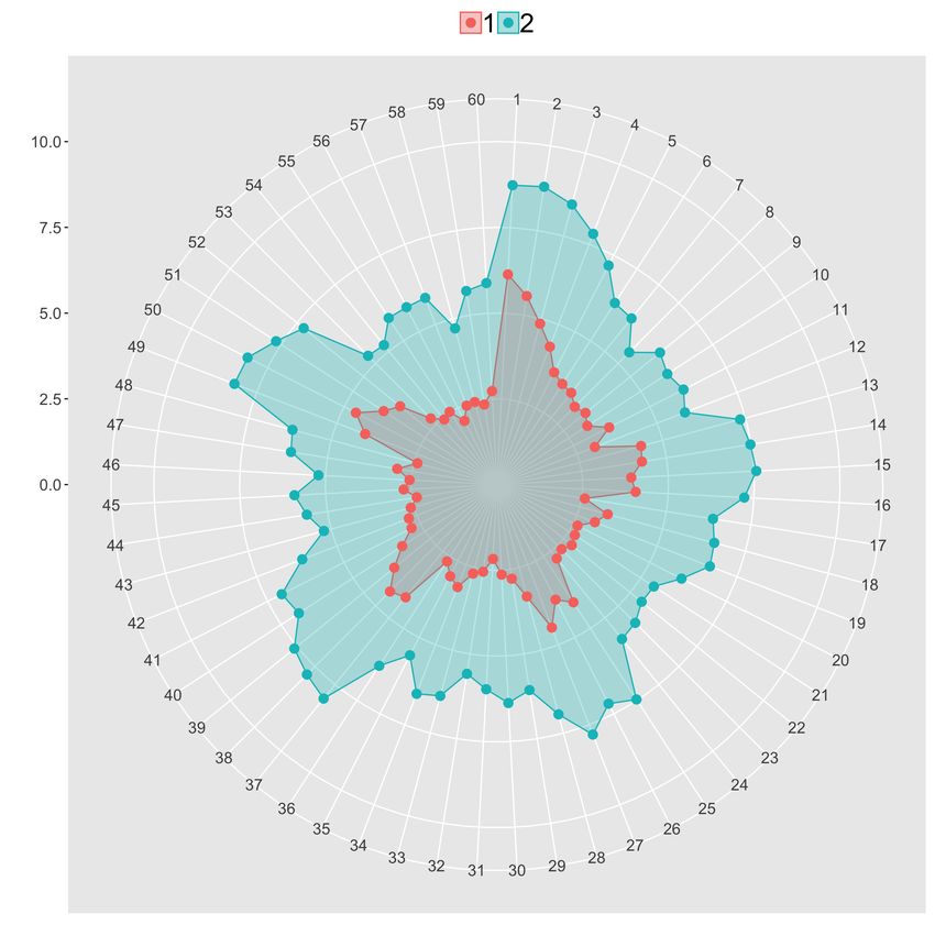
Exploring Age-Related Metamemory Di↵erences using Modified Brier Scores and
                            Hierarchical Clustering

                                 A Thesis by
                                Chelsea Parlett

                             Chapman University
                              Orange, California
                  Schmid College of Science and Technology
     Submitted in partial fulfillment of the requirements for the degree of
           Masters of Science in Computational and Data Sciences
                                   May 2019

                            Committee In Charge:
                       Professor Erik J. Linstead, Chair
                           Professor Rene German
                         Professor Elizabeth Stevens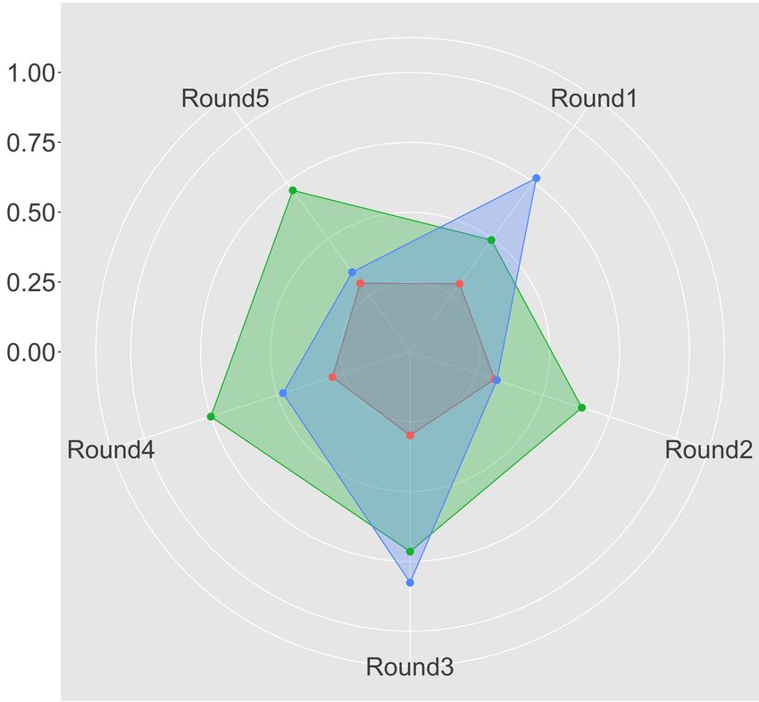
Exploring Age-Related Metamemory Di↵erences using Modified Brier Scores and
                          Hierarchical Clustering
                            Copyright c 2019
                            by Chelsea Parlett

                                    iii
ACKNOWLEDGMENTS
I would like to thank the National Science Foundation for supporting me with a
Graduate Research Fellowship (#1849569) I would also like to thank my committee
members, Dr. Erik Linstead, Professor Rene German, and Dr. Elizabeth Stevens
without whose support I could not have completed this thesis. Thank you also to
Open Psychology for allowing work published in their journal in this thesis.
ivVITA
Chelsea Parlett
EDUCATION
Master of Science in Computational and Data Science 2019
Chapman University Orange, California
Bachelor of Science in Psychology 2015
University of California, San Diego La Jolla, California
RESEARCH EXPERIENCE
Graduate Research Assistant 2017–2022
Chapman University Orange, California
Lab and Data Manager 2015–2017
University of California, Irvine Irvine, California
TEACHING EXPERIENCE
Graduate Teaching Instructor 2017–2022
Chapman University Orange, California
SELECTED HONORS AND AWARDS
Graduate Research Fellowship 2017–2022
National Science Foundation
vLIST OF PUBLICATIONS
LIST OF PUBLICATIONS
The benefits and challenges of implementing motiva- 2017
tional features to boost cognitive training outcome
Journal of Cognitive Enhancement
Predicting Individual Di↵erences in Working Memory 2017
Training Gain: A Machine Learning Approach
Cognitive Science
Applications of Supervised Machine Learning in Autism 2019
Spectrum Disorder Research: a Review
Review Journal of Autism and Developmental Disorders
Exploring the Relationship of Digital Information 2019
Sources and Medication Adherence
Computers in Biology and Medicine
Exploring Age-Related Metamemory Di↵erences using 2019
Modified Brier Scores and Hierarchical Clustering
Open Psychology
viABSTRACT
Exploring Age-Related Metamemory Di↵erences using Modified Brier Scores and
Hierarchical Clustering
by Chelsea Parlett
Older adults (OAs) typically experience memory failures as they age. However,
with some exceptions, studies of OAs’ ability to assess their own memory functions–
Metamemory (MM)– find little evidence that this function is susceptible to age-related
decline. Our study examines OAs’ and young adults’ (YAs) MM performance and
strategy use. Groups of YAs (N = 138) and OAs (N = 79) performed a MM task that
required participants to place bets on how likely they were to remember words in a
list. Our analytical approach includes hierarchical clustering, and we introduce a new
measure of MM—the modified Brier—in order to adjust for di↵erences in scale usage
between participants. Our data indicate that OAs and YAs di↵er in the strategies
they use to assess their memory and in how well their MM matches with memory
performance. However, there was no evidence that the chosen strategies were associ-
ated with di↵erences in MM match, indicating that there are multiple strategies that
might be e↵ective (i.e. lead to similar match) in this MM task.
viiTABLE OF CONTENTS
Page
ACKNOWLEDGMENTS iv
VITA v
LIST OF PUBLICATIONS vi
ABSTRACT OF THE THESIS vii
LIST OF FIGURES x
LIST OF TABLES xv
1 Introduction 1
1.1 How is MM Studied? . . . . . . . . . . . . . . . . . . . . . . . . . . . 2
1.2 Metamemory across the Lifespan . . . . . . . . . . . . . . . . . . . . 5
1.3 Calibration . . . . . . . . . . . . . . . . . . . . . . . . . . . . . . . . 8
1.4 Discrimination . . . . . . . . . . . . . . . . . . . . . . . . . . . . . . . 9
2 Methods 11
2.1 Participants . . . . . . . . . . . . . . . . . . . . . . . . . . . . . . . . 11
2.2 MM Task . . . . . . . . . . . . . . . . . . . . . . . . . . . . . . . . . 12
2.3 Word Selection . . . . . . . . . . . . . . . . . . . . . . . . . . . . . . 12
viii2.4 Analytical Approach . . . . . . . . . . . . . . . . . . . . . . . . . . . 20
2.4.1 Hierarchical Clustering . . . . . . . . . . . . . . . . . . . . . . 20
2.4.2 Application to our Dataset . . . . . . . . . . . . . . . . . . . . 21
3 Results 22
3.1 Bets and Correctly Recalled Words by Age . . . . . . . . . . . . . . . 22
3.2 mBrier Score by Age . . . . . . . . . . . . . . . . . . . . . . . . . . . 23
3.3 Hierarchical Strategy Clustering . . . . . . . . . . . . . . . . . . . . . 23
3.3.1 Two Strategy Clusters . . . . . . . . . . . . . . . . . . . . . . 24
3.3.2 Three Strategy Clusters . . . . . . . . . . . . . . . . . . . . . 25
3.4 mBrier Clusters . . . . . . . . . . . . . . . . . . . . . . . . . . . . . . 26
3.4.1 Two mBrier Clusters . . . . . . . . . . . . . . . . . . . . . . . 27
3.4.2 Three mBrier Clusters . . . . . . . . . . . . . . . . . . . . . . 28
3.4.3 mBrier Score by Strategy Cluster . . . . . . . . . . . . . . . . 29
4 Discussion 32
5 Future Work 37
Bibliography 38
Appendices 42
ixLIST OF FIGURES
Page
2.1 Figure 1. Scatterplot showing relationship between Gamma scores and
Modified Brier scores for this sample of data. . . . . . . . . . . . . . 16
3.1 A radar graph showing the average mBrier score for OAs (red) and YAs
(blue) across all 5 rounds of the MM task. Lower scores are better.
The scale on the left shows the progression of values from the center
of the circle, outwards. . . . . . . . . . . . . . . . . . . . . . . . . . . 23
3.2 Dendrogram from hierarchical clustering of betting strategy data at
the participant level showing the relative distances between clusters
(Height) and their hierarchical structure. The distance between clus-
ters visually represents how di↵erent clusters are from one another,
whereas the hierarchical arrangement shows how clusters are nested
within one another. . . . . . . . . . . . . . . . . . . . . . . . . . . . 24
x3.3 a. Radar Graph displaying bets for the two-cluster analysis. The
first cluster (low variation and low average bets) is shown in red, and
the second cluster (higher variation and higher average bets) is shown
in blue. The Radar graphs display the mean bets with each spoke
representing the bets for an item. Items are read clockwise from the
12 o’clock position onward. The scale on the left shows the progression
of values from the center of the circle, outwards. b. Barplot showing
counts of OAs (left) and YAs (right) for the two strategy clusters shown
in a. Cluster 1 represents low bets/low variance, Cluster 2 represents
high bets/high variance. . . . . . . . . . . . . . . . . . . . . . . . . . 25
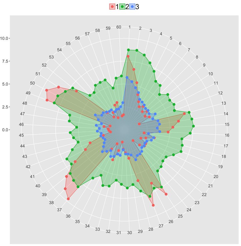
3.4 a. Radar Graph displaying bets for the three-cluster analysis. The
third cluster (low bets/ low variance) is shown in blue, and the second
cluster (high bets/high variance) is shown in green, and the first cluster
(high variance and more cyclical betting patterns) is shown in red. The
scale on the left shows the progression of values from the center of the
circle, outwards. b. Barplot showing distribution of OAs (left) and
YAs (right) between the three strategy clusters shown in a. . . . . . . 26
3.5 Dendrogram from hierarchical clustering of mBrier score data on the
participant level. The distance between clusters (Height) visually rep-
resents how di↵erent clusters are from one another, whereas the hierar-
chical arrangement shows how clusters are nested within one another.
. . . . . . . . . . . . . . . . . . . . . . . . . . . . . . . . . . . . . . . 27
xi3.6 a. Radar Graph displaying mBrier scores for the two-cluster analysis
across the five rounds. Cluster 1 (stable, low mBrier) is shown in red,
Cluster 2 (higher, less stable mBrier scores) is shown in teal. There are
five spokes in the mBrier radar graph with each spoke representing the
average mBrier scores for each round. mBrier can be between 0 (the
center of the graph) and 1 (the edge of the graph) with lower scores
being better. The scale on the left shows the progression of values from
the center of the circle, outwards. b. Barplot showing distribution of
OAs (left) and YAs (right) between the two mBrier score clusters shown
in a). . . . . . . . . . . . . . . . . . . . . . . . . . . . . . . . . . . . . 28
3.7 Figure 8. a. Radar Graph displaying mBrier scores for the three-cluster
analysis. Cluster 2 remained the same from the two-cluster analysis.
Cluster 1 (with stable, low mBrier scores across rounds) and 3 (blue)
were previously clustered together in the 2-cluster analysis (Cluster 1
shown in red, Figure 7a). Cluster 3 has more unstable mBrier scores
across rounds. The minimum mBrier score (0) is displayed at the
center, with increasing mBrier scores moving outward. The scale on
the left shows the progression of values from the center of the circle,
outwards. b. Barplot showing distribution of OAs (left) and YAs
(right) between the three mBrier clusters. . . . . . . . . . . . . . . . . 29
3.8 Mean plots of mBrier score by two (a) and three (b) cluster strategy.
Error bars represent +/- standard errors of the mean. . . . . . . . . . 30
xii3.9 Radar Graphs displaying the average mBrier score between the two (a)
and three (b) strategy cluster groups as a function of round. Lower
mBrier scores are closer to the center of the graph and represent better
performance. Overall, the average mBrier scores for each of the five
rounds is relatively similar for the two cluster groups. However, in the
three cluster groups, a clear pattern of lower (better) mBrier scores for
cluster 1 emerges. . . . . . . . . . . . . . . . . . . . . . . . . . . . . . 30
A.1 A barplot of the mean mBrier score for each mBrier Cluster (2 clus-
ters), split by age. This plot shows that which OAs and YAs may
still score di↵erentially, similar patterns emerge between OAs and YAs
with cluster 1 having lower mBrier scores, and cluster 2 having higher
mBrier scores for both Age groups. . . . . . . . . . . . . . . . . . . . 43
A.2 A barplot of the mean mBrier score for each mBrier Cluster (3 clus-
ters), split by age. This plot shows that which OAs and YAs may still
score di↵erentially, similar patterns emerge between OAs and YAs with
cluster 1 having lower mBrier scores, cluster 2 having higher mBrier
scores, and cluster 3 having scores in the middle for both Age groups. 44
A.3 A barplot of the mean mBrier score for each Strategy Cluster (2 clus-
ters), split by age. This plot shows that which OAs and YAs may still
score di↵erentially, similar patterns emerge between OAs and YAs with
scores being similar (but slightly lower for cluster 2) for both Age groups. 45
xiiiA.4 A barplot of the mean mBrier score for each Strategy Cluster (3 clus-
ters), split by age. This plot shows that which OAs and YAs may still
score di↵erentially, similar patterns emerge between OAs and YAs with
cluster 1 having lower mBrier scores, cluster 2 having midrange mBrier
scores, and cluster 3 having higher mBrier scores for both Age groups. 46
xivLIST OF TABLES
Page
2.1 Vignette 1 - Example of when Gamma (G) and mBrier lead to di↵erent
results. . . . . . . . . . . . . . . . . . . . . . . . . . . . . . . . . . . . 16
2.2 Vignette 2 - Example of when Gamma (G) and mBrier lead to di↵erent
results. . . . . . . . . . . . . . . . . . . . . . . . . . . . . . . . . . . . 17
2.3 Vignette 3 Example of where Brier and mBrier scores di↵er. . . . . . 19
3.1 Summary Statistics for OAs and YAs. . . . . . . . . . . . . . . . . . 22
A.1 Summary Statistics for Wordlist Characteristics. . . . . . . . . . . . . 42
A.2 Summary Statistics for Wordlist Characteristics. . . . . . . . . . . . . 42
xvChapter 1
Introduction
Imagine two older adults (OAs), Grandparents A and B, with a handful of grandchil-
dren each. Grandparent A is quite confident that he would be able to remember all
of his grandchildren’s birthdays and prepare birthday presents on time. Grandparent
B, on the other hand, is not as confident, and strategically marks down the birthdays
on her calendar.
This scenario illustrates the concept of metamemory (MM). MM, how one thinks
about one’s own memory ability, is multifaceted and various definitions exist. One
dominant view breaks MM down into three components: MM knowledge (a person’s
belief and thoughts about his/her own memory ability), memory monitoring (the as-
sessment of self’s likelihood of remembering something), and memory control (the
actions or strategies that the two previous components may lead to; see [12] [34]).
In our example, the Grandparents have varying beliefs (MM knowledge) regarding
their ability to remember birthdays, and as they monitored and assessed their own
beliefs, they arrived at two di↵erent control strategies to ensure successful outcomes
(Grandparent A doing nothing and Grandparent B spending the time to write the
1birthdays in her calendar). Another, not necessarily conflicting, view stems from the
classic MM paper by [15] that treats MM as having person, task, and strategy aspects.
While the person and strategy aspects map onto the knowledge and control elements
of the later conceptualization of MM, the task aspects refer to the kind of materials
that make it easier or harder for a person to remember. To clarify this distinction,
let us return to the Grandparents. It may be easier for Grandparent A to remember
the kids’ birthdays because he might not have as many grandchildren as Grandparent
B does. This is analogous to having a shorter list length of elements to remember,
which is an example of the task aspect of MM. Alternatively, at the person level,
Grandparent A’s family could have the habit of celebrating every birthday whereas
Grandparent B’s does not, thereby making birthdays more salient for Grandparent
A, resulting in Grandparent A being more confident in his ability to remember the
kids’ birthdays. Because of this confidence or metamemory knowledge, Grandpar-
ent A might not expend much energy to devise cognitive control or strategies for
remembering the grandchildren’s birthdays.
1.1 How is MM Studied?
Historically, due to the need or desire for meaningful, translational research for MM
that could be applied to real life, MM has been measured via self-report question-
naires. These questionnaires may touch upon real life scenarios that laboratory ex-
periments cannot simulate, such as reported self-appraisal of one’s own memory in
regular circumstances, the reported frequency of mnemonic strategy uses in the Mul-
tifactorial MM Questionnaire (MMQ; [46]), memory issues and/or changes associated
with healthy aging in the MM in Adulthood Questionnaire (MIA; [11]), or reports
of how often survey respondents forget things in di↵erent situations, the seriousness
2and consequences of such forgetfulness, and comparison of past and present memory
abilities in the Memory Functioning Questionnaire (MFQ; [16]). Although these ques-
tionnaires o↵er insights into the perceived memory abilities, or the MM knowledge,
of participants, the lack of objective measures of MM means they do not paint a com-
plete picture of people’s MM. Indeed, one consistent objective among MM research
is the push to go beyond merely making a judgment about the beliefs. Researchers
are equally interested in the accuracies of people’s MM beliefs. This central interest
may have practical value. If Grandparent A, despite the high level of confidence, were
terrible at remembering the birthdays, then his poor MM would mean missed birth-
days and, perhaps, disappointed grandchildren. If, on the other hand, Grandparent
B were actually excellent at remembering birthdays, then her underestimation of her
own memory ability would mean wasted time and, perhaps, an annoyed partner who
does not understand why she is always writing things down. If we had a clearer under-
standing of MM in aging and, in particular, what strategies were beneficial for whom,
then interventions could be tailored to meet the specific needs of individuals such as
Grandparents A and B. With the practical implications of MM, the focus of much
of the most recent research on MM has rested on monitoring and control with judg-
ment of learning (JOL) playing an important role [34]. In JOL tasks, participants are
typically asked to predict or estimate their memory performance. Though sometimes
defined as ”judgments of the likelihood of remembering recently studied items on an
upcoming test” ([34], p. 286, emphasis added), JOL tasks come in various forms.
For example, in the classic MM Battery [3], the Memory Estimation subtest that
closely resembles JOL asks participants to first predict how many items they would
remember from a list of 15. More recently, the field has shifted to examine JOL in
a more fine-grained manner. Rather than taking JOL on the overall test level (out
of all of your grandchildren, how many birthdays would you remember), researchers
are increasingly more interested in JOL at the item level (e.g., how likely are you to
3remember grandkid 1’s birthday, grandkid 2’s birthday, and so on). For example, in a
value-directed remembering task [7] [6], participants made JOLs by placing ”bets” on
word items that they thought they would remember later [28]. In the ”bets” version,
the JOL is essentially reduced to a yes/no decision. As mentioned earlier, monitoring
judgments by themselves form only one part of MM. The accuracy of these judgments
is of special interest. Yet accuracy of the JOLs has also been investigated in various
ways. In particular, researchers distinguish between relative accuracy (resolution) and
absolute accuracy (calibration; see [39] for a discussion). Say Grandparent A has to
go out shopping. For all the items they have to buy, Grandparent A is fairly confident
(e.g., 80% for remembering to get eggs and co↵ee to 100% rating for remembering to
get bread and milk) that they would remember items. Grandparent A would have
low calibration if they end up remembering only half of the shopping list. However,
the resolution would still be high if Grandparent A remembers the higher rated items
(in this case, bread and milk) more than the lower-rated items (in this case, eggs
and co↵ee). Empirically, how calibration scores are calculated varies depending on
the tasks and, therefore, no consistent calibration measurement exists. In the MM
Battery, for instance, the accuracy of the memory estimation subtest is calculated
via a somewhat arbitrary equation that weights the estimation with a separate list
before the actual recall test di↵erently from the estimation performed after the recall
test with yet another list of items [3]. In the recent value-directed tasks [28], because
the researchers’ purpose was to examine learning and strategies associated with item
values and the JOL was based on a simple yes/no decision, the calibration score could
only be calculated as a simple subtraction between actual number of items recalled
and the number of items on which a bet was placed. To date, no MM measure has
combined an objective MM task with a more fine-grained measure of participants’
own beliefs regarding their memory on any particular item, which is the aim of the
present work.
41.2 Metamemory across the Lifespan
Despite the di↵erential trajectories of various cognitive functions across the lifespan
with many memory-related functions showing age-related cognitive decline [37][17],
monitoring of MM has shown relatively little age e↵ects. Judgments of one’s ability to
remember things are notoriously difficult to measure in children and are only loosely
associated with other established constructs of MM such as strategy use [10]. As
people age, JOL measures have yielded much more reliable and consistent findings.
When it comes to the absolute accuracy of JOLs, adults, both young and old, tend
to be overconfident in their memory ability, often overestimating the number of items
they can remember, though this overconfidence seems to be much more inflated in
older adults (e.g. [9]; [28]). Moreover, this overconfidence may be more restricted
to single or initial block of trials, as there is also evidence that people can adjust
their calibration based on practice, sometimes attenuating their ratings to the point
of underestimating their ability in a phenomenon known as the underconfidence-with-
practice (UWP) e↵ect [25] [33] [41] [42].
Nevertheless, exceptions do exist for the robust UWP e↵ect (e.g., [28]; [33]). For
example, in the novel paradigm where participants made judgments to ”bet” on the
likelihood of remembering words based on their assigned values, neither older nor
younger adults became underconfident in later word lists [28]. It should be noted
that participants did indeed lower their number of bets in subsequent lists and became
more calibrated later on, but they never remembered more words than they bet on
[28]. This surprising lack of UWP could possibly be related to the novel ”betting”
paradigm where the binary yes/no decision and its accuracy could mean more or
fewer points in the final score. More research using this ”betting” paradigm would
therefore be beneficial in addressing some of these discrepancies.
5In addition to the initial overconfidence (albeit to di↵erent degrees) as measured
by absolute accuracy of their monitoring judgments, YAs and OAs display similar
patterns in monitoring relative accuracy (e.g., [20]; [19]; [14]; [42];[41]). For example,
in experiments with word-pair associative learning tasks with an explicit instruction
to form and use mental imagery for the word pairs, YAs and OAs based their JOLs
on whether they were able to successfully form an image (there was no age di↵erence
in imagery formation success), suggesting that both YAs and OAs were e↵ective in
monitoring their memory and strategy–image formation–use [14]. Similarly, gamma
correlation measures between JOLs and recall showed both YAs and OAs were equally
accurate in monitoring their memory of texts that they read [41].
Nonetheless, some earlier studies showed that OAs use monitoring to a lesser extent
than YAs do [13]; [40]. Additionally, even though the UWP e↵ect has been shown
in both age groups, sometimes OAs do not display the underestimation following
learning in the first trial [33]. In two experiments varying in the number of trials
(two trials only in experiment 1 and five trials in experiment 2), both YAs and OAs
overestimated their ability to remember word pairs during the first trial. However,
only YAs underestimated in the subsequent trials despite improvements in estimation
in both groups [33]. Beyond memory monitoring, it appears that YAs and OAs also
share methods of memory control or strategy [43], though some patterns of di↵erences
have also emerged. One classic method of investigating individuals’ cognitive control
or strategy use is to have participants make decisions regarding how they would al-
locate study time (e.g., [7]; [13]; [29]; [31], [32]). Across di↵erent studies that varied
the items in terms of difficulty or values (i.e. points awarded), two patterns emerged.
First, both YAs and OAs tended to prioritize easier items over harder items. Second,
both groups tended to prioritize high value items (e.g., [7]; [31]). However, OAs were
only likely to prioritize high value items that were also easy, whereas YAs were more
likely to prioritize high value items regardless of difficulty. This strategy di↵erence
6may be related to OAs’ lower memory self-efficacy [31]. Furthermore, studies demon-
strated that in learning a novel calculation task, OAs were less likely and slower to
switch from computing to retrieval strategy after repeated exposures to the same
stimuli [45]. Similarly, OAs were less likely to use retrieval as a strategy in noun-pair
associative learning tasks [35].
Thus, there seem to be subtle di↵erences between YAs and OAs in various aspects
of MM. Still, while the literature on MM in OAs has been developing for some time
now, there is no consensus regarding whether MM accuracy is impacted by aging, or
whether specific strategy use might play a role in any di↵erences or the lack thereof.
Furthermore, the literature appears fairly settled on the analytical approaches to
MM, employing straightforward deviation scores (e.g. Brier scores) for calibration,
and gamma correlations for resolution. Though the distinction of absolute versus
relative accuracy is imperative as they answer di↵erent questions pertaining to di↵er-
ent underlying metacognitive mechanisms (calibration pointing to judgment precision
and resolution to the correspondence between judgment and performance; see discus-
sion in [38]), the two measures may sometimes be at odds with each other, making an
overall inference about one’s MM difficult. For example, the robust UWP e↵ect exists
only for absolute accuracy (calibration); in the studies that demonstrated UWP in
calibration, participants’ resolution actually improves in later blocks or presentations
of trials (e.g., [24]). Considering the discrepant findings for calibration and resolu-
tion, a hybrid score may be useful in enhancing our understanding of MM and any
age-related di↵erences.
In order to conceptualize a ”new” approach to examine MM data, we will provide a
brief overview of the traditional, established methods in the following.
71.3 Calibration
Calibration, or absolute accuracy of the participants’ judgment as compared with their
actual performance, is typically a deviation score calculated via subtraction between
performance and judgment. Sometimes this subtraction is done in a straightforward
manner (e.g., [24]; [28]), while other times researchers calculate calibration using
equations that assign di↵erent weights to di↵erent lists (e.g., [3]). Among the varied
methods of calculating calibration, one measure (and its variants) stands out and is
most commonly used: Brier score (in MM literature, also known as calibration index;
see [38]):
n
1X
(acci joli )2 (1.1)
n i=1
Brier score measures the accuracy of probabilistic predictions [36] and provides the
precision of the confidence ratings (i.e. JOL). As the equation would suggest, a score
of zero corresponds to perfect accuracy (imagine JOL of 100% and performance of
100%, (100 100)2 = 0) and a score of one would be no accuracy (for example, a
100% JOL and 0% performance). Thus, counterintuitively, a higher score is consid-
ered having ”worse” MM using this index. The precise nature of this score also comes
with another caveat: individuals may have internal di↵erences in providing confidence
ratings. For example, cross-cultural studies of responses on Likert scale surveys re-
vealed that Asian and Asian American participants are less likely than other ethnic
groups to mark the extreme values (e.g., [2]; [8]). Thus, two people who are equally
confident may place their ratings based on di↵erent internal scales despite being given
the same scale of, say, 0-10, and Brier score does not correct for potential scaling dif-
8ferences. Resolution. This caveat of absolute scores can be addressed by examining
participants’ relative accuracy, or resolution. In MM research, gamma correlation
[30] is most commonly used to examine how well participants’ judgments correspond
with their actual performances (e.g., [22]; [23]). Because the correlation is largely
contingent upon variability among the ratings and performances, cases with extreme
scores (e.g., JOLs of all 100% or 0 or 100% accuracy) had to be excluded. While
this does not interfere with the theoretical validity of gamma, it can present practical
issues. In the current dataset, around 17% of gamma values were non-computable.
Because of this artifact and because participants’ performance tends to become bet-
ter throughout an experiment, resolution scores from one block to the next are often
calculated based on dwindling sample sizes (see for example [24]).
1.4 Discrimination
Yet another dimension in MM studies is the concept of discrimination, or the extent
to which confidence ratings between correct and incorrect items di↵er and can be
distinguished from one another [38]. Positive discrimination scores would indicate
that participants were more confident on items they recalled correctly than non-
recalled items. Conceptually, discrimination would be an ideal, additional construct
to measure metacognitive awareness. However, as the comparison would be between
correct and incorrect items (rather than within item JOL and accuracy comparison
as in the case of calibration), discrimination scores are calculated at the aggregate
level and may be less precise.
Resolution and discrimination scores have been instrumental for theory development
(e.g., cue-utilization theory), providing insights into the mechanisms with which peo-
ple make confidence ratings or monitor their own knowledge or memory. Yet, the
9addition of a hybrid score may address some practical concerns, ranging from some-
thing as trivial as answering participants’ questions of ”I feel like I did worse later.
Am I right?” to something more substantial as addressing the cases when the data
do not allow for proper, meaningful calculation of resolution scores. Having a hybrid
score that takes into account both the precision and association between judgment
and performance may be helpful as a first-step presentation of a birds-eye view of the
metamemory scheme before breaking down into the details of the mechanisms with
which people monitor their knowledge and memory.
To address these issues, our study employs a novel version of a MM task that allows
for a more detailed assessment of participants’ own beliefs regarding their memory
on any particular item. Further, we use machine learning methods to understand
nuances in the data that may shed light on these issues in a way that traditional
analytical methods have not been able to in the past. To do so, we take advantage of
the fine-grained nature of the individual word bets. Rather than having participants
estimate their memory at the list level, providing judgment ratings at the item level
allows for a more nuanced understanding of MM. We seek to answer the question of
whether older and younger adults di↵er in their MM, as measured by a new hybrid,
mBrier score, and how their strategy use might a↵ect the new hybrid MM mBrier
scores.
10Chapter 2
Methods
2.1 Participants
Data was collected from 233 YAs and OAs. Healthy OAs were recruited through flyers
distributed in community centers in Southern California, and they received monetary
compensation for their participation. YAs were undergraduate social science stu-
dents who participated for course credit. Data for all participants were collected in
a controlled laboratory setting. Sixteen (n = 13 OAs; n = 3 YAs) participants were
excluded due to technical difficulties, or missing/corrupted data. Listwise deletion
was used for missing data due to the restrictions imposed by our clustering methods.
The final analytical sample consisted of 79 OAs (mean age = 73.72, SD = 4.91; 62
women; vocabulary score 22.08, SD = 3.89) and 138 YAs (mean age = 20.71, SD =
2.38; 101 women; vocabulary score 15.44, SD = 3.65).
112.2 MM Task
This MM task was adapted from a similar computerized task by [28]. Participants
were presented with five rounds of 12 words, shown one at a time with the overall
instruction to remember as many words as possible. After each word was shown for
3 seconds, participants were given up to 5 seconds to place a bet (a version of a JOL)
between 0 and 10 points. After seeing the 12 words, participants were asked to recall
as many words as possible by typing them into the computer. They were told that
if they correctly remembered a word, the bet for their word would be added to their
score. If they did not remember a word, their bet would be subtracted from their
score. Participants were given unlimited time to recall the words of each list. Extra
words that were entered (i.e. words not in the list) were not counted in their score.
Correct spelling and tense were required in order to be counted as correct, however
participants were allowed to correct misspellings if they noticed them. After each
round, participants were presented with their score–the MM score–for that round
before proceeding to the next round of 12 words. The experimenter further explained
that the objective is for the participants to get as high of a score as possible.
2.3 Word Selection
One version of the word list was adapted from [28]. For the other, we combined the
sets of words from the English Lexicon Project [1], which contains the Hyperspace
Analogue to Language (HAL) word frequency norms [26] from the HAL corpus of
about 131 million words, with databases containing valence [48] and imageability [4].
Only words with ratings for these lexical features remained in the potential stimuli
pool. We further limited the stimuli to 4-7 letter words that are nouns, neutral in
12terms of emotional valence (1 standard deviation around the median of valence), high
frequency (1 standard deviation around the 75th percentile of the frequency index),
and neutral imageability (1 standard deviation around the median). To create the
second version, we randomly selected 60 of the words and split them into 5 lists. As
mentioned earlier, each word list contains 12 words (therefore each version has 60
words). Within sets, every participant received the same five lists in the same order.
However, participants were randomly assigned to receive either set A or B.
While there is a significant di↵erence between the number of correctly recalled words
between the two versions (p = 0.02, Bayesian analysis did not provide strong support
for a di↵erence, with a BF10 = 0.986) as well as di↵erences in frequency, valence,
concreteness, imageability and length (p’s < 0.01, BF10 ’s > 13, all BF10 ’s but valance
> 192), there was not a significant di↵erence between the average bets nor mBrier
scores (score described below), arousal, nor polysemy (BF10 < 0.827). Exact summary
statistics are available in the Supplementary materials. Within each version, there
is no significant e↵ect of round (1-5) or interaction between version and round in
any word characteristics, signifying that within versions, the word lists for round do
not di↵er significantly. Furthermore, for all clusters examined in this paper, there
was no statistically significant di↵erence between the distributions of version between
clusters (i.e. clusters did not have significantly di↵erent proportions of either version)
Bayesian analysis agreed, finding no strong evidence that there is a di↵erence in
distribution between the two versions (all BF10 ’s < 0.86 ). mBrier Score. The MM
score as described above, is a measure of both MM and raw memory capacity, and,
along with the number of words recalled irrespective of bets, has been used as the
primary dependent variable for that measure [28].
Participants with high scores must both have good MM and be able to remember
some words, since the only way to gain points is to correctly recall a word. While this
13specific combined measure is useful, there is also a need to tease apart the memory
capacity and MM components of this score. This paper o↵ers a di↵erent, supplemen-
tary score, called the modified Brier score (mBrier) that o↵ers better insight into the
MM component of the task. We will provide vignettes and general descriptions of
when mBrier o↵ers better or more practical scores over two traditional measures of
metamemory performance: Gamma and a traditional Brier score.
The mBrier score is a hybrid score (for a description of hybrid scores, see [38]). Its
calculation follows the traditional Brier score calculation. However, instead of using
binary JOLs, or even continuous percentages (e.g. the numerical response to ”what
is the probability that you will remember this word?”), the mBrier score uses a scaled
and ranked transformation of the JOLs. Bets/JOLs ranked from 1 to n, with n being
the number of non-zero bets/JOLs.
n
1X
(acci Rjoli )2 (2.1)
n i=1
where Rjoli is the ranked jol,where rank is calculated after excluding all jols=0. In
order to calculate the ranked JOLs, first, all items that were given a JOL of 0 are
excluded, and left as 0’s. Then, the remaining items’ JOLs are ranked. The resulting
ranked JOLs are then scaled by the maximum rank in order to get a probability
between 0 and 1. Traditionally, many MM studies have used the Goodman-Kruskal
gamma as a measure of resolution. The formula for gamma is show below for ease of
reference.
(Ns Nd )
G= (2.2)
(Ns + Nd )
14Where Ns is the number of concordant word pairs (e.g. where the bet of word A is
higher than the bet of word B, and the accuracy of word A is higher than word B)
and Nd is the number of discordant pairs (e.g. where the JOL of word A is higher
than the JOL of word B, and the accuracy of word A is lower than word B). In this
calculation, all pairs where either the JOL or accuracy are the same (e.g. if a subject
recalled or did not recall both words, or gave the same JOL for both words) are
discarded.
While Gamma is generally a useful resolution measure, it can be lower when JOLs are
not binary [22]. There have also been concerns about reliability of Gamma (e.g., [21];
[44]) and how Gamma appeared unrelated to task difficulty and individual di↵erences
[27]. The lack of reliability could be related to how many item pairs are excluded in the
Gamma calculation. This is of particular concern, as patterns are not noncomputable
at random, rather, certain patterns are more likely to be excluded, such as bet/JOL
perseveration.
This is increasingly impactful towards the extremes of the Gamma score (-1 and 1).
The modified Brier score is highly negatively correlated with Gamma (r = -0.71 in
this sample; correlation is negative because Gamma and mBrier are coded di↵erently
with high Gamma scores and low mBrier scores both indicating good performance),
however it shows the most di↵erence at the extremes. The negative correlation is due
to the fact that Gammas score from -1 to 1 with 1 being the highest performance,
while Brier scores go from 0 to 1 with 0 being the highest performance. An example
from our dataset of where the modified Brier score allows better di↵erentiability
between MM performance is presented below.
Participants A and B (data is pulled from our dataset) both have a Gamma of 1 (the
highest score possible), however they score very di↵erently using a modified Brier
score (0.585 and .183 respectively).
15Figure 2.1: Figure 1. Scatterplot showing relationship between Gamma scores and
Modified Brier scores for this sample of data. .
Table 2.1: Vignette 1 - Example of when Gamma (G) and mBrier lead to di↵erent
results.
ID word a b c d e f g h i j k l G mBrier
bet
A 10 10 10 10 10 10 5 10 10 10 10 10
(jol) 1 0.585
acc 1 1 1 1 0 0 0 0 0 0 0 0
bet
B 10 10 3 3 3 1 1 1 1 2 1 1
(jol) 1 0.183
acc 1 1 1 0 0 0 0 0 0 0 0 0
16Table 2.2: Vignette 2 - Example of when Gamma (G) and mBrier lead to di↵erent
results.
ID word a b c d e f g h i j k l G mBrier
bet(jol) 2 1 1 4 3 4 4 4 3 4 3 3
C -1 0.679
acc 1 1 1 0 0 0 0 0 0 0 0 0
bet(jol) 1 5 4 1 3 1 2 10 6 5 5 10
D -1 0.57
acc 1 1 1 1 1 1 1 0 0 0 0 0
There is a clear di↵erence in the performance of these two participants, yet this
di↵erence is not captured by Gamma. Participant A gives maximum JOLs for all but
1 word, and only recalls 4 of them. However, because 11 out of the 12 JOLs are the
same (10), the number of pairs that Gamma considers for Participant A is severely
limited. Since there is only one low JOL, we can only consider pairings that include
the word associated with this JOL. Since it was not recalled, we also must exclude
pairings with words that were not recalled. In this case, it leads to a situation in which
the one non-recalled word with a low JOL (”owl”), is only compared to recalled words.
This leads to exclusively concordant pairs (owl-girl, owl-frog, owl-bus, owl-apple), and
thus a high gamma. However, examining Participant A’s strategy reveals that for the
most part, they are not good at appropriately assigning JOLs, they happened to have
one case in which they did appropriately assign a lower JOL to a non-recalled word.
On the other hand, Participant B also has a Gamma of 1, however it’s clear from the
strategy of Participant B, that they have a better grasp of giving appropriate JOLs.
While they did recall one low JOL word (”help”), overall their JOLs are high for
recalled words and low for non-recalled words. Their betting pattern allows Gamma
to reflect this, unlike with Participant A. Similarly, two participants, C and D (again,
pulled from our dataset), both have a Gamma of -1. However, their scores using our
score are quite di↵erent (0.679 and 0.570 respectively).
In the case of Participant D, the Gamma score and our score coincide: both give
it an almost maximally low score (-1 is the lowest possible Gamma, indicating that
17JOLs are inversely correlated with accuracy. If you give a low JOL, you’re most likely
to recall the word. However, Participant C got the same Gamma as Participant D,
however, looking at their performance, it’s possible to see that while they were more
likely to remember words with low JOLs, the magnitude of the inappropriateness of
their JOLs is smaller, reflected in our score of -0.55. Di↵erentiating between these two
patterns is important, and the authors believe that a single score reflecting potential
discrepancies is useful, even though it is valuable to look at calibration and resolution
separately and does not replace Gamma. Our hybrid score represents a comprehensive
overview of performance that allows for finer grained di↵erentiation. This is especially
valuable at the extreme ends of Gamma Scores. Importantly, and specifically to our
task and dataset, Gamma has an undefined value when either all JOLs are the same, or
all accuracies are the same (either all words recalled or none recalled). Unfortunately,
this scenario happens often, specifically, in about 17% of rounds in our sample. Since
full feature vectors are needed to perform good hierarchical clustering, using Gamma’s
reduces the data set from 217 to 139, signaling that at least 78 of the original 217
participants had at least one noncomputable gamma value. Brier Scores. Brier scores
are the mean squared error of JOLs (taken as a probability) compared to accuracy
of recall or recognition. Brier scores also are computable on an item-by-item level.
A comparison with mBrier which is also computable on an item-by-item level is
discussed below. The formula for Brier score shown below are sometimes referred to
as the absolute accuracy (calibration) index (see [38]).
n
1X
(fi oi )2 (2.3)
n i=1
where fi is the preditcted probability of success between 0 and 1. And oi is the
18Table 2.3: Vignette 3 Example of where Brier and mBrier scores di↵er.
ID word a b c d e f g h i j k l Brier mBrier
bet(jol) 4 4 4 4 4 2 2 2 2 2 2 2
E 0.23 0.18
acc 1 1 1 1 0 0 0 0 0 0 0 0
bet(jol) 10 10 10 10 10 0 0 0 0 0 0 0
F 0.09 0.18
acc 1 1 1 1 0 0 0 0 0 0 0 0
accuracy,0 or 1. As a measure of calibration, Brier scores treat JOLs as probabilities
of recall. However, di↵erent participants often use the scale in this task di↵erently.
This is especially important in this task, where JOLs were framed as ”bets”. In order
to account for this, the modified Brier score uses the scaled rank of the JOL rather
than the unranked JOL in its calculation. The following vignette is an example of
when mBrier is helpful, and was chosen specifically to elucidate more clearly when
mBrier is beneficial. Two participants, Participants E and F (data extracted from
our study), could have a similar MM performance, but because of their di↵erent uses
of the JOL scale, have di↵erent Brier Scores.
By using a modified, ranked Brier score, information above and beyond calibration
alone can be observed. In the above case, both participants would receive a modified
Brier score of 0.18. In this respect, our modified score shares characteristics with
both calibration and resolution. Again, this is especially important in the current
task because JOLs were framed as bets rather than percentages. Derived from the
classic absolute accuracy index (i.e. Brier score), our modified score utilizes rank
order, resulting in scores that would highlight relative accuracy. Our score aims to
account for di↵erences in scale usage by using the ranked value of bets.
192.4 Analytical Approach
For strategy clusters, the raw bets for all 60 (5x12) words were used, resulting in
a 60-dimensional vector. For mBrier clusters, the mBrier score for each round was
used, resulting in a 5-dimensional vector.
2.4.1 Hierarchical Clustering
Hierarchical Agglomerative clustering was used to cluster both the raw betting and
mBrier data at the participant level. Hierarchical Clustering reveals the hierarchical
structure of groups within the data, allowing for more both coarse and fine-grained
analyses of di↵erent strategies and calibration improvements. In Hierarchical Agglom-
erative clustering–also called bottom-up clustering–each data point starts o↵ as its
own singleton cluster. Each cluster is then continually merged with the next closest
cluster until all the data points are in one cluster [47]. Multiple linkage criteria exist
to determine the distance between two clusters. In this analysis, complete-linkage
was used. The results of Hierarchical Agglomerative clustering can be shown visually
using a dendrogram that shows the nested structure of the clusters. Hierarchical clus-
tering allows for the examination of multiple levels of nested clusters. Hierarchical
clustering was performed on 60 dimensional vectors of participant’s bets across all 60
trials. For mBrier scores, 5 dimensional vectors of average mBrier scores by round
were used. Using unsupervised machine learning methods like hierarchical clustering
can help detect naturally occurring groups in the data. For example, participants
who use di↵erent betting strategies, or participants who have similar trajectories
for improvement of their mBrier scores. We believe that looking at the hierarchical
structure of clusters will be beneficial because it will allow for the examination of
similarities between di↵erent clusters. This will allow researchers to look at as coarse
20or fine-grained clusters as necessary. In some situations, it may be beneficial to look
a high level, coarser clusters, especially in the case that clusters are used as a basis
for targeted interventions. However, looking at lower level, more fine-grained clusters
may be useful when looking at individual di↵erences. The highest level clusters (2
and 3 clusters) were examined in the present paper in order to pull out high level
di↵erences between di↵erent strategies and performances.
2.4.2 Application to our Dataset
Data for all participants, regardless of age were clustered on both their bets and their
mBrier scores over time. This helps distinguish groups of participants who have either
similar strategies when completing the task, or similar improvements over time, i.e.
across the 5 rounds. The betting strategy groups are of special interest since it will
allow us to a) define and describe di↵erent strategies used on this task, and then b)
investigate whether OAs use di↵erent strategies than YAs. We can also test whether
there is a di↵erential e↵ect of strategy use on mBrier score (i.e. whether certain
strategies are associated with higher mBrier). Understanding the di↵erent strategies
and their association with lower mBrier may pave the way for interventions that teach
strategies that are helpful for OAs.
21Chapter 3
Results
Summary Statistics for the data are shown in Table 3.2. Data were analyzed using R
(3.4.3 Kite-Eating Tree) and JASP (JASP Team (2018). Version 0.8.3.1).
3.1 Bets and Correctly Recalled Words by Age
Average bets across all 60 words was not significantly di↵erent between OAs and
YAs (t(215) = 1.769, p = 0.078, d= 0.25; BF10 = 0.661). However, as expected, the
average number of correctly recalled words was significantly di↵erent between OAs
and YAs, with OAs remembering less words (t(215) = 11.06, p < 0.001, d = 1.56 ;
BF10 = 3.651e19).
Table 3.1: Summary Statistics for OAs and YAs.
N Bets Words Recalled mBrier
OAs 79 4.12(2.99) 3.67(1.98) 0.44(0.23)
YAs 138 4.6(3.39) 5.99(1.94) 0.39(0.14)
Note. The average scores across all lists (12 words per list) for bets (JOLs), words
recalled, and mBrier score are provided. Standard deviations are given in parentheses.
22Figure 3.1: A radar graph showing the average mBrier score for OAs (red) and YAs
(blue) across all 5 rounds of the MM task. Lower scores are better. The scale on the
left shows the progression of values from the center of the circle, outwards.
3.2 mBrier Score by Age
OAs had a significantly worse average mBrier score than YAs (t(215)= -7.681, p <
0.001, d = -1.084, BF10 = 1.152e10). The hybrid mBrier scores across rounds–instead
of overall averages–can be seen plotted in Figure 3.1. In order to test whether age
di↵erences emerge over time, we ran a repeated measures ANOVA with age group as
between subject factor and round as within factor, which revealed a significant age
group round interaction, agreeing the with Bayes Factor for this analysis (F(4,860)
= 4.53, p = 0.001; BFinteraction = 9.77).
3.3 Hierarchical Strategy Clustering
This dendrogram reveals less separable clusters (compared to dendrograms with more
density at the bottom) since the dendrogram is denser in the middle range of the y-
axis than at the bottom. Typically, clusters that are cohesive and separate (i.e. items
23Figure 3.2: Dendrogram from hierarchical clustering of betting strategy data at the
participant level showing the relative distances between clusters (Height) and their
hierarchical structure. The distance between clusters visually represents how di↵er-
ent clusters are from one another, whereas the hierarchical arrangement shows how
clusters are nested within one another.
in a cluster are very close to other items in that cluster, and far away from items in
other clusters) will have dendrograms that are denser at the lower range of the y-axis
(i.e. more connections will be made in the lower range of the y-axis).
3.3.1 Two Strategy Clusters
First, we look at the two highest level clusters: Cluster 1 consisted of relatively low
bets and low variance between bets. Instead, Cluster 2 consisted of high bets, and
higher variance. These patterns can be seen more clearly in the Radar graph in Figure
3.3a.
Figure 3.3b displays the distributions of OAs (left) and YAs (right) between these
two clusters. A chi-square test of independence revealed no significant di↵erence in
2
strategy usage between OAs and YAs ( (1) = 0.5575,p =0.4553; BF10 0.249; Fisher’
24[a] [b]
Figure 3.3: a. Radar Graph displaying bets for the two-cluster analysis. The first
cluster (low variation and low average bets) is shown in red, and the second clus-
ter (higher variation and higher average bets) is shown in blue. The Radar graphs
display the mean bets with each spoke representing the bets for an item. Items are
read clockwise from the 12 o’clock position onward. The scale on the left shows the
progression of values from the center of the circle, outwards. b. Barplot showing
counts of OAs (left) and YAs (right) for the two strategy clusters shown in a. Cluster
1 represents low bets/low variance, Cluster 2 represents high bets/high variance.
s Exact Test,p = 0.3815 ). Fisher’s Exact Test was run for all analyses since some
cluster assignments resulted in an expected cell value smaller than 5.
3.3.2 Three Strategy Clusters
Clustering the betting strategy data into three clusters again yielded the same cluster
with relatively low bets and low variance between bets, which we will now refer to
as Cluster 3 (blue). And Cluster 2–with high bets, and higher variance–remained
largely the same (green). Cluster 1, is characterized by extreme variance, and a
cyclical pattern between each of the 5 rounds (note the 5 spikes in red in Figure
3.4a). Clusters 1 and 3 in this analysis were previously clustered together in the
2-cluster analysis above. These patterns can be seen more clearly in the Radar graph
in Figure 5a.
25[a] [b]
Figure 3.4: a. Radar Graph displaying bets for the three-cluster analysis. The
third cluster (low bets/ low variance) is shown in blue, and the second cluster (high
bets/high variance) is shown in green, and the first cluster (high variance and more
cyclical betting patterns) is shown in red. The scale on the left shows the progression
of values from the center of the circle, outwards. b. Barplot showing distribution of
OAs (left) and YAs (right) between the three strategy clusters shown in a.
The distributions of Older and YAs between these clusters is shown in Figure 3.4b.
Both a chi square test of independence and a Fisher’s exact test again did not re-
2
veal a significant di↵erence in strategy usage between OAs and YAs ( (2)= 2.268,p
=0.3217;BF10 =0.105 ;Fisher’s Exact Test,p = 0.3276).
3.4 mBrier Clusters
The present paper will focus on analysis with 2 and 3 clusters, however, analyses
using 49 clusters can be made available by emailing the authors.
The dendrogram for the hierarchical clustering of mBrier scores is dense at the bottom,
revealing more separable clusters since points tend to join together in the lower range
of the y-axis. On the lefthand side of the graph, a smaller cluster that is far away
from the rest of the data can be seen (as it connects to the rest of the data very high
on the y-axis).
26Figure 3.5: Dendrogram from hierarchical clustering of mBrier score data on the
participant level. The distance between clusters (Height) visually represents how
di↵erent clusters are from one another, whereas the hierarchical arrangement shows
how clusters are nested within one another.
3.4.1 Two mBrier Clusters
In the 2-Cluster analysis, the first cluster, Cluster 1 has a relatively stable mBrier
score over all 5 rounds, and mBrier scores were relatively low (indicating higher
performance) compared to the other cluster. Cluster 2’s mBrier scores were slightly
more variable and characterized by many ups and downs, and on average were higher
(worse) than the mBrier scores of Cluster 1. These patterns can be seen in the radar
graph in Figure 3.6a.
The distribution of OAs and YAs between these two clusters was significantly di↵erent
2
( (1)= 28.00,p < 0.001; BF10 = 314124;Fisher’ s Exact Test,p < 0.001), suggesting
that OAs and YAs tend to di↵erentially adjust their mBrier scores across the five
rounds. Compared to YAs, OAs are more likely to be in Cluster 2, which has higher,
less stable mBrier scores (cf. Figure 3.6b). This pattern is also supported by the
di↵erence in mBrier as a function of age seen in Figure 3.1.
27[a] [b]
Figure 3.6: a. Radar Graph displaying mBrier scores for the two-cluster analysis
across the five rounds. Cluster 1 (stable, low mBrier) is shown in red, Cluster 2
(higher, less stable mBrier scores) is shown in teal. There are five spokes in the
mBrier radar graph with each spoke representing the average mBrier scores for each
round. mBrier can be between 0 (the center of the graph) and 1 (the edge of the
graph) with lower scores being better. The scale on the left shows the progression
of values from the center of the circle, outwards. b. Barplot showing distribution of
OAs (left) and YAs (right) between the two mBrier score clusters shown in a).
3.4.2 Three mBrier Clusters
In the 3-Cluster analysis, Cluster 1 from the 2-Cluster analysis remains the same.
Cluster 2 from the 2-cluster analysis breaks into Clusters 2 and 3. The clusters are
visualized in Figure 3.7a. Cluster 1, the red regular pentagonal cluster, again contains
those with relatively low, stable mBrier scores across all five rounds. Both Cluster 2
(green) and 3 (blue) show higher (worse performance) overall mBrier scores, as well
as more variation between rounds.
The distribution of OAs and YAs between these 3 clusters, shown in Figure 3.7b, was
2
significantly di↵erent ( (2) = 32.19,p < 0.001; BF10 = 64135; Fisher’s exact test,
p < 0.001), again suggesting that OAs and YAs tend to di↵erentially adjust their
mBrier scores over time.
28You can also read