Evaluating Reordering Strategies for Cluster Identification in Parallel Coordinates
←
→
Page content transcription
If your browser does not render page correctly, please read the page content below
Eurographics Conference on Visualization (EuroVis) 2020                                                                                                                   Volume 39 (2020), Number 3
M. Gleicher, T. Landesberger von Antburg, and I. Viola
(Guest Editors)

                                    Evaluating Reordering Strategies
                             for Cluster Identification in Parallel Coordinates
                     Michael Blumenschein1                   , Xuan Zhang2             , David Pomerenke1                , Daniel A. Keim1              , and Johannes Fuchs1
                                                 1 University    of Konstanz, Germany                         2 RWTH      Aachen University, Germany

      (a) Medium clutter, Similar                            (b) High clutter, Similar                        (c) Medium clutter, Dissimilar                        (d) High clutter, Dissimilar

Figure 1: A dataset with three clusters and two different clutter levels is sorted by similarity (a–b) and dissimilarity (c–d) of neighboring axes
pairs. Clusters are more salient when arranging dissimilar dimensions next to each other. We show that in cluttered datasets, participants are
more accurate and more confident when performing cluster identification tasks on such a layout.
         Abstract
         The ability to perceive patterns in parallel coordinates plots (PCPs) is heavily influenced by the ordering of the dimensions.
         While the community has proposed over 30 automatic ordering strategies, we still lack empirical guidance for choosing an
         appropriate strategy for a given task. In this paper, we first propose a classification of tasks and patterns and analyze which
         PCP reordering strategies help in detecting them. Based on our classification, we then conduct an empirical user study with
         31 participants to evaluate reordering strategies for cluster identification tasks. We particularly measure time, identification
         quality, and the users’ confidence for two different strategies using both synthetic and real-world datasets. Our results show that,
         somewhat unexpectedly, participants tend to focus on dissimilar rather than similar dimension pairs when detecting clusters, and
         are more confident in their answers. This is especially true when increasing the amount of clutter in the data. As a result of these
         findings, we propose a new reordering strategy based on the dissimilarity of neighboring dimension pairs.
         CCS Concepts
         • Human-centered computing → Empirical studies in visualization;

1. Introduction                                                                                              fluences the perception of visible patterns [SKKAJ15]. This prob-
Parallel coordinates plots (PCPs) [Ins85, Ins09b] are a popular and                                          lem is particularly given in PCPs, as line crossing and overplot-
well-researched technique to visualize multi-dimensional data. Di-                                           ting distort salient structures. Therefore, the community has pro-
mensions are represented by vertical, equally spaced axes. Data                                              posed a multitude of enhancements, such as sampling [ED06], edge
records are encoded by polylines, connecting the respective val-                                             bundling [MM08], interactive highlighting [MW95], and the usage
ues on each axis. PCPs have been applied to practical applica-                                               of transparency [JLJC05] to reduce the impact of visual clutter.
tions of various domains [JF16], such as finance [AZZ10], traffic
                                                                                                                The ordering of axes plays a fundamental role in the design of a
safety [FWR99], and network analysis [SC∗ 05]. As discussed by
                                                                                                             PCP and has a strong effect on the overall pattern structure [JJ09].
Andrienko and Andrienko [AA01], PCPs are suited for a multitude
                                                                                                             In contrast to data preprocessing, sampling, dimension filtering,
of analysis tasks, such as cluster, correlation, and outlier analysis.
                                                                                                             and other enhancements, reordering does not remove data from the
  Compared to other visualizations for multi-dimensional data (e.g.,                                         PCP [PWR04, PL17], but changes the visual structure among neigh-
RadVis [HGM∗ 97], MDS and PCA projections, scatter plots, and                                                boring axes. Depending on the user’s analysis goal, some patterns
scatter plot matrices), PCPs have the advantage to trace data records                                        are more interesting than others [DK10]. As a result, more than 30
and patterns across a large set of dimensions. Empirical studies have                                        different ordering strategies have been developed by the community
shown that PCPs outperform scatter plots in clustering tasks, outlier,                                       to support a multitude of tasks. Some of these strategies group simi-
and change detection [KAC15], but are less suited for correlation                                            lar dimension pairs [ABK98], try to avoid line crossings [DK10],
analysis [LMvW10, HYFC14] and value retrieval [KZZM12].                                                      or put the most important dimensions first [YPWR03]. However,
   A major challenge of visualizations is visual clutter, which in-                                          our community lacks empirical guidance and recommendations for

© 2020 The Author(s)
Computer Graphics Forum © 2020 The Eurographics Association and John
Wiley & Sons Ltd. Published by John Wiley & Sons Ltd.

This is the accepted version of the following article: M. Blumenschein, X. Zhang, D. Pomerenke, D.A. Keim, J. Fuchs (2020), Evaluating Reordering Strategies for Cluster Identification in Parallel Coordinates,
Computer Graphics Forum, 39(3), which has been published in final form at http://onlinelibrary.wiley.com. This article may be used for non-commercial purposes in accordance with the Wiley Self-Archiving
Policy [http://www.wileyauthors.com/self-archiving].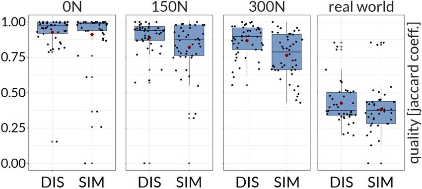
Blumenschein et al. / Evaluating Reordering Strategies for Cluster Identification in Parallel Coordinates

choosing an appropriate strategy for a given task [BBK∗ 18]. In this            complexity of the data [TAE∗ 11]. More importantly, optimizing the
paper, we address this limitation by summarizing the state-of-the-art           axes ordering to highlight a particular pattern may even obstruct
in axes reordering strategies, as well as presenting a first empirical          other patterns [JJ09], which are of relevance in a different scenario.
user study that measures the performance of two ordering methods                Therefore, it is vital to carefully choose an appropriate strategy to
for cluster identification in PCPs. Our study focuses on cluster anal-          arrange the axes in parallel coordinates.
ysis as the majority of ordering strategies are designed for this task.            More than 30 reordering strategies have been developed (see Sec-
   We claim two main contributions. First, we provide guidance                  tion 3), many of which follow similar concepts but differ in their im-
in selecting reordering strategies based on their intended patterns.            plementation affecting, for example, the runtime and quality of the
Many existing algorithms follow similar concepts but differ in their            results. Quality metrics and layout algorithms for PCPs have been
implementation. To support users, we introduce a classification                 summarized before: Heinrich and Weiskopf [HW13] give a compre-
of the existing layout algorithms, group them according to their                hensive overview of the state-of-the-art for PCP research, including
inner workings, and summarize their intended patterns and meta-                 manual and automatic reordering approaches. Bertini et al. [BTK11]
characteristics. For more practical support, we implemented a set of            and Behrisch et al. [BBK∗ 18] summarize quality metrics to optimize
14 strategies in JavaScript and made them along with the source code            the visual representation. Ellis and Dix [ED07] discuss reordering
available on our website for testing: http://subspace.dbvis.de/pcp.             from a clutter perspective. While Behrisch et al. [BBK∗ 18] group
   Second, we measure the performance of two reordering strategies              the quality metrics by their analysis task, the literature still misses a
for cluster identification tasks by an empirical user study with 31             summary of the different PCP patterns and a discussion on which
participants. We realized that the often proposed similarity-based              reordering algorithms favor or avoid particular patterns [TAE∗ 11].
axes arrangement (e.g., [ABK98, YPWR03, AdOL06]) is not always                  In our paper, we close this gap by introducing a classification along
the most effective solution to identify clusters. As shown in Figure 1,         with a characterization of the reordering algorithms.
arranging axes with a high dissimilarity next to each other produces
more salient clusters, in particular in cluttered and noisy datasets.
                                                                                2.2. Evaluation of Axes Reorderings and Empirical Studies
A reason for this effect is that lines with strong slopes are moving
closer together, making clusters visually more prominent [PDK∗ 19].             There is a lack of empirical studies to measure the performance
To find out whether this arrangement is more useful than a similarity-          of specific axes orderings for different analysis tasks [JF16]. Most
based layout, we conducted a user study and measured performance                strategies are “evaluated” using examples of synthetic or real-world
with respect to cluster quality, completion time, and users’ confi-             data (see Table 1) instead of comparing it to previous approaches.
dence using synthetic and real-world datasets. Our results show that            Exceptions are the works by Ferdosi & Roerdink [FR11] and Tatu
participants tend to focus on dissimilar axes pairs when selecting              et al. [TAE∗ 11], which compare the resulting orders with competing
clusters and are more accurate and confident when doing so.                     approaches. However, no feedback from real users is provided.
   As a secondary contribution, we provide a benchmark dataset                     Many reorderings claim to be useful for cluster analysis, but we do
with 82 synthetic and real-world datasets for clustering analysis.              not know yet which patterns are most effective in identifying clusters.
For reproducibility, we make all our material and results, statistical          There is no user study that compares different reorderings for clus-
analysis, and source code publicly available at https://osf.io/zwm69.           ter identification in particular or different analysis tasks in general.
   The remainder of this paper is structured as follows: In the next            Therefore, we want to push PCP reordering towards an empirically-
section, we summarize important related work. Then, in Section 3,               driven research field by evaluating two axes reordering techniques
we survey existing reordering strategies for PCPs and classify them             for cluster identification. The works most closely related to ours are
based on their intended patterns and inner workings (first contribu-            the empirical studies by Holten & van Wijk [HvW10] (measuring
tion). Afterwards, in Section 4, we describe our user study design              response time and cluster identification correctness for nine PCP
and report the statistical analysis results in Section 5 (second contri-        variations), Kanjanabose et al. [KAC15] (measuring response time
bution). Finally, we discuss our findings and derive design consider-           and clustering accuracy in PCP, scatter plots, and classical tables),
ations for axes orderings in cluster identification tasks.                      and the study by Johansson et al. [JFLC08] evaluating clutter thresh-
                                                                                old for the identification of patterns. However, none of these studies
2. Background and Related Work                                                  consider different axes orderings as an independent variable.
In the following, we summarize the challenges of axes reordering,
the results of existing user studies, and the relation of automatic             2.3. Relation to Interactive and Semi-Automatic Analysis
ordering to interactive and semi-automatic analysis support.                    Besides axes reordering, countless enhancements have been devel-
                                                                                oped to support the understanding of patterns in parallel coordi-
2.1. Challenges of Axes Reordering of Parallel Coordinates                      nates. A comprehensive overview is out of the scope of this paper
Linear ordering of an n−dimensional dataset in PCPs faces two main              but can be found in the surveys by Ellis & Dix [ED07], Bertini
challenges. First, computing and evaluating all dimension permuta-              et al. [BTK11], Heinrich & Weiskopf [HW13], and Behrisch et
tions is computationally expensive. Ankerst et al. [ABK98] show                 al. [BBK∗ 18]. Many techniques involve users within an interac-
that the ordering of axes according to some useful objective function           tive exploration workflow or combine the representation with au-
is NP-complete. Therefore, the exhaustive search for a useful order-            tomatic algorithms for pattern detection. Examples are the usage
ing is tedious, even for a modest number of dimensions [PWR04].                 of clustering algorithms [FWR99, JLJC05, Mou11], automatic sam-
Second, the usefulness of a particular ordering highly depends on               pling techniques [ED06], and interactive highlighting [MW95]. In-
the analysis task of the user [DK10, PL17], and is influenced by the            selberg [Ins09a], and Hurley & Oldford [HO10] propose to clone

                                                                                                                                                      © 2020 The Author(s)
                                                                                     Computer Graphics Forum © 2020 The Eurographics Association and John Wiley & Sons Ltd.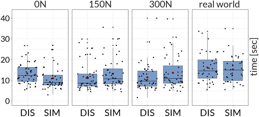
Blumenschein et al. / Evaluating Reordering Strategies for Cluster Identification in Parallel Coordinates
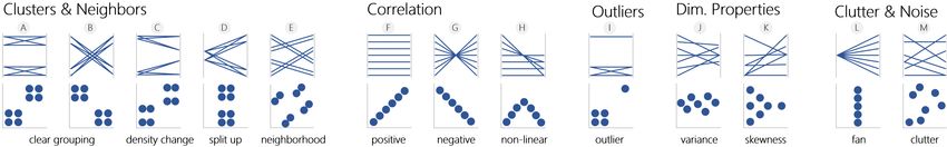
Figure 2: Comparison of visual patterns in parallel coordinates and their scatter plot representation.
and arrange dimensions such that all pairwise permutations are visi- Outliers I . Outliers squeeze the majority of PCP lines together,
ble, similar to a scatter plot matrix. Based on this initial view, the resulting in a cluster-like pattern, hiding the underlying structure.
user can then start the exploration. Dimension Properties J – K . show patterns of dimensions, or-
While the usefulness of such interactive and visual analytics dered by variance and skewness. The lines’ slope indicates whether
approaches have been shown in many user studies, they are facing patterns stay consistent (parallel) or change across axes.
two challenges: First, most algorithms rely on sensitive parameters Clutter & Noise. Randomly distributed data without a clear pattern
which influence the quality of the result. For example, k-means is considered noise or clutter in the data. The lines in the PCP cross
clustering [HKP11] requires the number of clusters as user input, without any particular structure M . The fan pattern L describes a
which is typically unknown for a new dataset. Second, interactive
cluster transitioning into clutter, a special case of density change C .
exploration and highlighting are difficult if users do not know what
Our selection of patterns is based on the work by Dasgupta &
they are searching for, and the initial configuration of a PCP does not
Kosara [DK10], Wegman [Weg90], Heinrich & Weiskopf [HW13,
show (parts of) interesting patterns. Often, this results in trial-and-
HW15], and Zhou et al. [ZYQ∗ 08]. The cluster variations (i.e., pat-
error interactions, in which patterns are only detected ‘by accident’.
terns A – D ) are inspired by Pattern Trails [JHB∗ 17], which intro-
This is particularly true if the dataset contains a large number of
duces a taxonomy of pattern transitions between multi-dimensional
dimensions, and relevant patterns only exist in smaller subspaces.
subspaces. These patterns can be adapted to PCP, as two neighbor-
Therefore, we need methods to give analysts good starting condi- ing axes show a transition between one-dimensional subspaces. Fi-
tions for their (interactive) analysis. Hereby, an important aspect is nally, we add variance J and skewness K , which is produced by
the arrangement of axes, as it significantly changes the visual pat- the algorithms described in [LHZ16, SCC∗ 18, YPWR03]. We limit
terns among neighboring axes [JJ09]. In our paper, we provide a our patterns to 2D PCPs and ignore patterns in 3D PCPs (e.g., dis-
categorization of reordering algorithms and their intended patterns, cussed in [PL17, AKSZ13]. We also consider only patterns among
which helps analysts to make an educated selection. the two axes. Multi-dimensional patterns can be achieved by con-
catenating multiple two-dimensional patterns.
3. Classification of Reordering Strategies
This section addresses two questions: Which patterns are empha- 3.2. Ordering Strategies
sized by which reordering strategy? And which algorithms have To find ordering strategies, we took the 502 references of recent state-
been implemented to solve the reordering problem? Before answer- of-the-art reports [HW13, JF16, BBK∗ 18] and combined it with 497
ing these questions, we provide an overview of important patterns. papers resulting from a search on the ACM, IEEE Xplore, EG, and
DBLP digital library (see keywords and details in the supplementary
3.1. Visual Patterns material). We recursively scanned references and excluded papers
Figure 2 shows five groups of the most common patterns in parallel that (1) did not propose an automatic axes ordering strategy (e.g.,
coordinates and their representation in scatter plots: purely interactive approaches), (2) “just” apply a reordering method
which has been proposed before, or (3) approaches which do not
Clusters & Neighbors A – E . Typical cluster structures show focus on “standard” parallel coordinates (e.g., 3D PCPs). Using this
one or more groups of dense lines in a similar direction. While A & approach, we collected 18 papers with 32 different strategies.
B seem similar in scatter plots, the visible structure in PCP differs Table 1 summarizes all reordering strategies, grouped by their
significantly. C shows clusters that change their density (cluster ordering concept: strategies transforming the reordering into an op-
compactness) and D , a cluster that splits up into sub-clusters. timization problem (Section 3.3), implementing efficient or sophisti-
Structures, preserving neighborhood information, are a special cated algorithms (Section 3.4), and approaches focusing on proper-
case of clusters. A (small) set of data records similar (close) to each ties of single dimensions (Section 3.5). For each approach, we indi-
other in one dimension are also similar in the neighboring dimension, cate the favored patterns, the involved axes, and the performed eval-
which results in groups of parallel lines E . uation to show the usefulness (see caption of Table 1 for details).
Correlations F – H . Positive and negative correlations look simi-
lar in a scatter plot. However, the PCP patterns differ: lines are par- 3.3. Optimization Problem and Objective Functions
allel for positive F , and in a star-like pattern for negative correla- The largest group of reordering strategies transforms the axes ar-
tions G . Variations of non-linear correlations may look different in rangement into an optimization problem. These approaches measure
both scatter plots and PCPs. H shows only an example as the pat- the quality of a particular ordering by an objective function, which is
tern depends on the type and degree of change in both dimensions. then either minimized or maximized by an optimization algorithm.
© 2020 The Author(s)
Computer Graphics Forum © 2020 The Eurographics Association and John Wiley & Sons Ltd.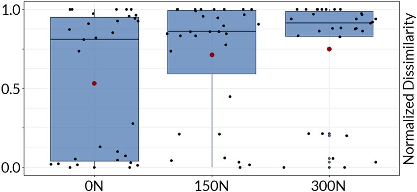
Blumenschein et al. / Evaluating Reordering Strategies for Cluster Identification in Parallel Coordinates
Table 1: Reordering Classification summarizing the inner workings of reordering strategies for parallel coordinates. For each technique, we
mark if it favors or avoids a particular pattern, if present in the data. Empty cells mean that the technique is not designed for this pattern and
produces/avoids it primarily by change. Approaches are grouped by their concept and sorted according to the similarity of patterns that they
favor and avoid. Additionally, we indicate the number of dimensions that are taken into account for the reordering and mark techniques which
can be combined with dimension filters and subspace analysis. Finally, we mark the evaluation type used in the paper. Due to space limitations,
we only show the name of the first author.
Patterns: algorithm favors or avoids ⊗ pattern, or it depends on data properties and algorithm parameters .
Axes considered for ordering: each dimension separately ( ), two neighboring dimensions ( ), or the majority of dimensions ( ).
The technique can be combined with: dimension filters (DR) and subspace analysis (S).
Evaluation: case study or example , comparison with other techniques , and empirical study .
A B C D E F G H I J K L M
Reordering Technique Axes Dim. Eval.
Tatu (no label) [TAE∗ 11] ⊗
Tatu (given label) [TAE∗ 11] ⊗
Long (class consist.) [Van15] ⊗ ⊗
Objective Function & Optimization Algorithm
Zhou (cluster trace) [ZYYC18] ⊗ ⊗
Peltonen (neighbor) [PL17] ⊗ ⊗
Dasgupta (overpl.) [DK10] ⊗
Dasgupta (parall.) [DK10] ⊗ ⊗ ⊗
Ankerst (similar) [ABK98] ⊗ ⊗ ⊗
Yang (similarity) [YPWR03] ⊗ ⊗ ⊗ DR +S
∗
Xiang (clus. interac.) [XFJ 12] ⊗ ⊗
Ankerst (correl.) [ABK98] ⊗ ⊗ ⊗
Artero (clutter) [AdOL06] ⊗ ⊗ ⊗ ⊗
F Blumenschein (dissimil.) ⊗ ⊗ ⊗
Dasgupta (cross.) [DK10] ⊗ ⊗
Dasgupta (angle) [DK10] ⊗ ⊗
Dasgupta (mut. i.) [DK10] ⊗
Makwana (struc.) [MTJ12]
Peng (outlier) [PWR04]
Dasgupta (entropy) [DK10] ⊗
Dasgupta (diverg.) [DK10] ⊗
Johansson (cluster) [JJ09] ⊗ DR
Reordering Algorithm
Ferdosi (subspace) [FR11] ⊗ DR +S
Huang (set theory) [HHJ11] ⊗
Artero (similar) [AdOL06] ⊗ ⊗ ⊗ DR
Johansson (correl.) [JJ09] ⊗ ⊗ ⊗ DR
Lu (non-lin. corr.) [LHH12] ⊗
Johansson (outlier) [JJ09] ⊗ DR
∗ ⊗ –
Schloerke (class) [SCC 18]
Dimension QM
∗ ⊗ –
Schloerke (outlier) [SCC 18]
Lu (svd) [LHZ16] ⊗ DR
Yang (variance) [YPWR03] ⊗ DR +S
Schloerke (skewn.) [SCC∗ 18] ⊗ –
© 2020 The Author(s)
Computer Graphics Forum © 2020 The Eurographics Association and John Wiley & Sons Ltd.Blumenschein et al. / Evaluating Reordering Strategies for Cluster Identification in Parallel Coordinates
3.3.1. Objective Functions Measuring Cluster Structures tion density, highlighting many line crossings and inverse relation-
Tatu et al. [TAE∗ 09,TAE∗ 11] argue that clusters consist of lines with ships. The metric does not favor specific patterns, but results in busy,
a similar position and direction (patterns A , B , and D ). The au- but very readable charts, according to the authors [DK10]. The met-
thors take a rendered image of a PCP and apply a Hough space trans- ric by Makwana et al. [MTJ12] differs from previous metrics. The
formation [Hou62]. Each PCP line segment is mapped into one point authors propose to order dimensions such that neighboring axes con-
within the Hough space. The point’s location represents the position tain lines with different slopes, resulting in cluttered M PCPs.
and slope of the line segment. The objective function measures dense Peng et al. [PWR04] interpret outliers as data points that do not
areas (clusters) of points in the Hough space. Long [Van15] first belong to a cluster. They measure the ratio of outliers against the
computes a centroid for all given clusters. Then for each data record, number of data points. When maximized, outliers are highlighted
the nearest centroid is identified (using the area between the lines as (pattern I ), when minimized, outliers will not be highlighted.
similarity function), and the objective function measures the ratio
of correctly classified records. Cluster patterns A and B are high- 3.3.4. Optimization Algorithms for Objective Functions
lighted, while a cluster split D is avoided. Zhou et al. [ZYYC18] Except for [AdOL06], all approaches measure the quality be-
aim at clusters that can be followed across neighboring axes ( A tween neighboring axes and use the average as the objective
and B ). They compute a hierarchical clustering on every dimension function. To minimize or maximize this function, various heuris-
and use the cluster similarity as quality. Dasgupta & Kosara [DK10] tics are applied: Random swapping (particularly useful for very
introduce seven different metrics, known as pargnostics. A metric large datasets) [YPWR03, PWR04], Ant-optimization [ABK98],
aiming for clusters like A and B is overplotting. It measures the A*Search [TAE∗ 09, TAE∗ 11], Nearest-neighbor-based [PWR04],
number of pixels that are not visible due to overlapping lines. When Branch and bound optimization [DK10, MTJ12], Non-linear opti-
maximizing this measure, there is a high information loss, but a mization algorithm [PL17], and Backtracking [ZYYC18].
high-density of lines, i.e., clusters. Finally, Xiang et al. [XFJ∗ 12]
try to avoid intersecting clusters B by measuring the crossing of
clusters among axes. This results in horizontal cluster structures A . 3.4. Reordering by Algorithms
Peltonen & Lin [PL17] aim to preserve the neighborhood distri- The second class of strategies arranges dimensions based on lay-
bution of records (pattern E ). The objective function measures the out algorithms. Compared to optimization procedures, this has two
similarity of nearest neighbors for all data records across two dimen- advantages: (1) Algorithms which approximate the understanding
sions. Clusters like A and B are a special case of neighborhood of an objective function, lead to more efficient but potentially less
relationships and are therefore considered as well. accurate results (e.g., [LHH12, AdOL06, JJ09]). (2) Objective func-
tions are typically defined only between neighboring axes. Using
3.3.2. Similarity-based Metrics for Clusters and Correlation more advanced algorithms (e.g., based on subspace clustering) lead
The main idea of the following approaches is to arrange similar di- to PCP, which aims for higher-dimensional patterns [FR11].
mensions next to each other. This results in cluster- and correlation
patterns. The definition of similarity differs across the techniques. 3.4.1. Algorithms for Efficient Reordering
Ankerst et al. [ABK98] use a Euclidean distance and Pearson cor- Artero et al. [AdOL06] and Johansson & Johansson [JJ09] speed
relation for the similarity computation. The approach by Yang et up the similarity and correlation-based axes arrangement, originally
al. [YPWR03] follows the same idea. However, they structure the di- presented by Ankerst et al. [ABK98]. Both algorithms are identical,
mensions into a hierarchy using a hierarchical clustering algorithm except for the similarity function. Artero et al. use a Euclidean dis-
to highlight also clusters in subspaces of the dataset. The hierarchi- tance, Johansson & Johansson, a Pearson correlation coefficient. The
cal structure also helps to speed up the computation time, as each algorithm starts with the most similar dimension pair in the center
subtree can be sorted independently. Depending on the similarity of the PCP. Iteratively, the next most similar dimension is appended
function, and whether the objective function is minimized or maxi- to the left or right side. While this approach is efficient, it also has
mized, these approaches aim for the patterns A , B , F , and G . the advantage that the most salient structure (the most similar di-
Other metrics try to order axes such that lines are most parallel mensions) typically ends up close to the center of the PCP, which
or diverging a lot. These patterns can help to identify correlations, users are most attracted to [NVE∗ 17]. Lu et al.’s approach [LHH12]
but may also favor clusters to some extent. Artero et al. [AdOL06] orders dimensions based on correlation. They use the nonlinear cor-
propose the total length of poly-lines as metric for pattern F . Simi- relation coefficient (NCC), which is sensitive to any relationship
larly, there are four pargnostic [DK10] measures: (1) Maximize the F – H (not only linear ones) and can be used for partial similarity
number of line crossings to identify inverse relationships G in the matching as well [ABK98]. The proposed algorithm combines the
data. (2) Maximizing G the angle of crossings. (3) Maximizing par- ordering by (non-linear) correlations together with an importance
allelism, resulting in less cluttered PCPs, which highlight positive driven arrangement. The first (left) axis in the PCP is chosen based
correlations F . (4) Maximizing the mutual information, which mea- on the highest singular value after a singular value decomposition
sures the dependency between variables, i.e., optimizing for positive (SVD, highest contribution of the dataset). Afterwards, all dimen-
F , negative G , and non-linear correlations H . sions are arranged from left to right according to their similarity of
the NCC. The approach by Huang et al. [HHJ11] maximizes the uni-
3.3.3. Objective Functions for Clutter and Outliers form line crossings of clusters. Their approach is based on Rough
The pargnostic metric maximizing divergence results in fan pattern Set Theory [Paw12], and the algorithm sorts the dimensions based
L , which helps to identify cluster-to-noise relationships. Maximiz- on alternating sizes of high and low cardinality of the equivalence
ing the entropy of neighboring axes corresponds to a high informa- classes, leading to cluster patterns A – C .
© 2020 The Author(s)
Computer Graphics Forum © 2020 The Eurographics Association and John Wiley & Sons Ltd.Blumenschein et al. / Evaluating Reordering Strategies for Cluster Identification in Parallel Coordinates
3.4.2. Subspace Algorithms for Higher-dimensional Structures the study by Netzel et al. [NVE∗ 17], who found out that people pay
Ferdosi & Roerdink [FR11] use a subspace search algo- the most attention to the center part of a PCP. (3) The evaluation of
rithm [FBT∗ 10] to identify higher-dimensional clusters with pat- novel reordering algorithms is primarily achieved by use cases and
terns A – D . The quality of one subspace is based on a density dis- example applications. We are not aware of empirical user studies
tribution. Subspaces containing multiple clusters that are clearly sep- that compare different orderings for a particular analysis task. With
arated are considered of high quality. First, the algorithm computes our paper, we want to close this gap and provide the first empirical
all one-dimensional subspaces and arranges the one with the highest study to evaluate ordering approaches for a particular analysis task.
quality on the very left of the PCP. Afterwards, all two-dimensional
subspaces, which contain the first subspace, are computed, and the 4. User Study Design: Reordering for Cluster Identification
highest rank is attached as the second axis. The algorithm continues Our reordering classification in Table 1 reveals that the majority of
until all dimensions are part of the PCP, or no more subspace can be strategies are designed to support cluster analysis. Therefore, we
computed. Johansson & Johansson [JJ09] apply the MAFIA algo- select this task as the focus of our user study. In particular, we want
rithm [NGC01], resulting in a set of subspaces, along with cluster to assess the performance of cluster identification, as this is the
structures and quality measures. The ordering algorithm then finds foundation for more sophisticated clustering analyses.
the longest sequence of connected variables shared by all detected For cluster analysis, similarity-based layouts are proposed most
subspace clusters. It starts with all dimensions of the first subspace often. Clusters, if present, can be followed across many axes, as
(no specific ordering). Further subspaces are iteratively added based algorithms try to minimize their variance. However, this strategy
on their quality, but only if they share a substantial set of dimen- does not necessarily highlight clusters. This is especially true if the
sions with the current PCP. The authors use the same algorithm to dataset contains noise or clutter, as shown in Figure 1a. While we
identify patterns with (multi-dimensional) outliers (pattern I ). can identify the clusters, they are visually less salient. In this paper,
we define the term clutter as data records that do not contribute to
3.5. Reordering by Dimension-wise Quality Metrics a particular pattern (e.g., randomly distributed), often also called
The third group of reordering techniques computes a quality for each noise. Cluttered datasets often end up in visual cluttered PCP due to
dimension separately ( ) and sort the axes accordingly. Assuming many line crossings and overplotting.
the quality can be computed efficiently, reordering can be done in Due to experiments with our implemented reordering algorithms,
linear time. The techniques can also be extended by dimension filter- we realized that polylines and clusters with strong slopes are visu-
ing (e.g., considering only dimensions with a quality above a thresh- ally more prominent than horizontal ones. There are two reasons, as
old). Relations between dimensions are not considered. Therefore, discussed by Pomerenke et al. [PDK∗ 19]: (1) With an increasing
patterns may be scattered in different parts of the PCP [PL17]. slope, the distance between polylines decreases, and less whitespace
Lu et al. [LHZ16] sort the axes based on each of their contribu- (background) is visible. Hence, neighboring lines have higher con-
tions to the dataset. They compute an SVD and sort the dimensions trast. (2) Compared to horizontal lines, diagonal lines need more
according to their singular values. Yang et al. [YPWR03] propose pixels to encode a single data point, resulting in a low data-to-ink-
a similar approach but sort the dimensions by variance. Both re- ratio [Tuf01]. Both geometric effects make sure that neighboring
orderings result in similar patterns ( J – L ). However, Lu et al.’s lines are more easily perceived as a group or cluster. Interestingly,
approach takes the distribution of the entire dataset into account. strong slopes are produced when dimensions are ordered by dissim-
Schloerke et al. [SCC∗ 18] propose three different dimension met- ilarity. An example can be found in Figure 1c. It shows the same
rics: (1) They use skewness for reordering, resulting in a K pattern. data as in 1a, but with strong slopes due to reordering. Often this re-
(2) The dimensions are sorted by one of the Scagnostics [WAG05] sults in a zig-zag-like pattern, which makes the visual representation
measures. In particular, the Outlying measure is useful to highlight more complex but also ends up in more salient cluster structures.
outliers in the data (pattern I ). (3) Finally, the authors order the di-
mensions such that existing clusters or classes are separated as well 4.1. Hypotheses
as possible. They compute an ANOVA on every dimension based We address the question, ‘whether there is a difference between a
on a given set of class labels and order the dimensions based on the similarity-based (SIM) and dissimilarity-based (DIS) axes ordering
F-statistic. Intuitively, the dimensions are ordered according to how for a cluster identification task’. If yes, ‘which ordering should
well the given clusters are separated (patterns A – C ). be used, and why?’ As the majority of real-world datasets contain
noise and clutter, we also want to investigate its influence generally,
3.6. Summary and in combination with the axes ordering. Hence, we analyze two
In Table 1, we provide an overview of 32 different reordering ap- independent variables: ordering method and clutter level.
proaches to arrange the axes of parallel coordinates. During our To measure the performance, we use three dependent variables:
analysis, we made a few observations: (1) Many reordering algo- (i) time to identify clusters, (ii) quality of manually selected clusters
rithms follow similar concepts, but differ in their implementation based on similarity to ground truth clusters, and (iii) the confidence
and the applied metric. The main reason for this is that axes reorder- of the users after the cluster identification. Additionally, we analyze
ing is computationally complex, and more efficient approaches are axes-pairs which help to identify the clusters. In particular, we
necessary for interactive applications. (2) There seems to be a differ- investigate whether users select clusters in similar or dissimilar axes
ent understanding of the most important area in a PCP. While some pairs. For our study, we formulate the following three hypotheses:
reordering approaches try to put the most important dimensions up- H1. With an increasing amount of clutter, the cluster identification
front, others try to arrange them in the center. This is in line with performance drops (independent of the ordering) as cluster structures
© 2020 The Author(s)
Computer Graphics Forum © 2020 The Eurographics Association and John Wiley & Sons Ltd.Blumenschein et al. / Evaluating Reordering Strategies for Cluster Identification in Parallel Coordinates
are less salient in the PCP plot. Therefore, we expect users to be the performance in real settings. We selected the datasets based
(a) slower, (b) less accurate, and (c) less confident. on common usage in PCP reordering (i.e., by choosing datasets
H2. Without clutter, users perform better in a cluster identification used in the techniques described in Table 1). Hence, the number
task when the axes are ordered by SIM instead of DIS as clusters of dimensions and records differ compared to synthetic datasets.
can be followed more easily. In particular, we expect users to be Dimensions range between 4 − 13, and the number of records be-
(a) faster, (b) more accurate, and (c) more confident with SIM. tween 32 − 515. Examples are the wine, mt-cars, and ecoli
dataset. If present, we removed categorical dimensions and out-
H3. With clutter, users perform better in a cluster identification
liers. We used Ward’s method [WJ63] to retrieve a hierarchical clus-
task when the axes are ordered by DIS instead of SIM as clusters
tering and a visual inspection to determine the clusters in the data.
are visually more prominent. In particular, we expect users to be
(a) faster, (b) more accurate, and (c) more confident with DIS.
4.3. Implementation
4.2. Benchmark Dataset and Ground Truth To compare the ‘optimal’ SIM and DIS layout, we used Ankerst
et al.’s reordering algorithm [ABK98] with an exhaustive search to
To evaluate our hypotheses, benchmark datasets with ground truth
find the axes ordering. For the SIM layout, we used the Euclidean
information and increasing clutter levels are needed. We are not
distance and minimized the sum of distances. For DIS, we used the
aware of such datasets for a cluster identification task. Therefore, we
same algorithm but maximized the distances. We pre-computed the
developed our own benchmark, consisting of ten popular real-world,
orderings for all datasets in advance. To run the study, we developed
and 72 synthetically created datasets along with the ground truth
a web application that is available at http://subspace.dbvis.de/pcp-
information. We make our dataset available in order to overcome
study. The parallel coordinates plots have a size of 960 × 500 pixels
the limitation of publicly available benchmark datasets [SNE∗ 16]
and use color for the polylines to separate them from the axes which
and to support the evaluation of PCP enhancements and reordering
are colored in black. We did not add any design variations to the chart
techniques in the future. For comparison, we also present a PCP with
(i.e., transparency, or edge bundling) to avoid confounding factors.
each dataset and reordering strategy in the supplementary material.
Synthetic datasets. We limit the dimensionality of all synthetic 4.4. Tasks and Data Randomization
datasets to eight. This allows us to create complex cluster structures Our study consisted of 21 trials per participant, which are grouped
while keeping the expected time for the study in a reasonable time into three tasks that build on top of each other. The tasks were
frame. We alternated the number of clusters between one and four executed in increasing difficulty: Tasks 1, 2, and 3. Between two
and varied the structures of the clusters – ranging from linear clusters trials of a task, we showed a white screen with the term ‘break time’,
towards a high variance on all scales of the different axes. and participants had to click a button to continue with the next trial.
Using the PCDC tool [BHvLF12], we manually created 24 base
datasets ({1, 2, 3, 4} clusters × 6 variations) which fulfill the fol- 4.4.1. Task 1 (Similarity of Axes-Pairs)
lowing properties: (i) clusters are clearly visible and separated from We wanted to find out which visual structures support users in a
each other, (ii) there is only one clustering result per dataset, (iii) cluster identification task. In particular, we were interested whether
each cluster is present in all eight dimensions, and (iv) no outliers users find neighboring axes with a high similarity or dissimilarity
are added as they would distort the existing patterns [AA01]. In up more useful. In each trial, we showed the participants a PCP in
to two dimensions, we merged two or more clusters such that partici- which the number of clusters had to be counted. Users selected the
pants need to investigate all dimensions to identify a cluster. To make number which they identified using four radio buttons (i.e., 1, 2, 3,
the clusters comparable across datasets, we kept the cluster size con- 4) and a can’t tell option. After the selection was confirmed, we
stant with small randomization in the range of 45 − 50 data points showed a single radio button between each neighboring axes (see
and vary the diameter of every cluster in each dimension randomly Figure 3 left) and asked the participants to select the pair which
in the range 0.15 − 0.30. All dimensions are normalized in 0.0 − 1.0. supported them best. Only one pair could be selected.
Next, we designed different clutter levels. Pomerenke et Randomization. We randomly picked three synthetic datasets with
al. [PDK∗ 19] show that random clutter (randomly and equally dis- a different number of clusters. In the first trial, we showed 0N clutter,
tributed records in all axes) produces visible patterns in PCPs which in the second 150N, and finally 300N (increasing difficulty). As we
look similar to clusters (Ghost clusters). In order to not accidentally are interested in whether participants prefer (dis-)similar neighbor-
include ‘fake patterns’ in our dataset, but also be fair w.r.t. random ing axes, we arranged dimensions such that the PCP contains both
clutter, we use a mixture of 30% random and 70% linear clutter (for similar and dissimilar axes pairs. To do so, we computed the simi-
every record: uniform and random distribution in one dimension larity of neighboring axes using the Euclidean distance and used the
± 0 − 0.15 in all other dimensions). Using several pilot experiments, maximal variance of similarities (MaxVar) as an objective function
this setting seemed to be complex enough, but also without any unde- (see example in Figure 4). In summary:
sired patterns. For each base dataset, we created two copies with dif- 3 levels of clutter (0N, 150N, 300N) ×
ferent clutter levels, one with 150 (150N), one with 300 data points
(300N). We used the same clutter datasets for all base datasets to 31 participants =
make them comparable and ensure we do not encode additional pat- 93 trials in total
terns in some of the datasets. After finalizing all 72 datasets (24 Post-processing. We collected the time to identify the number of
base datasets ×{0N, 150N, 300N}), we randomized the order of clusters along with the similarity value of the selected axes pair. For
the records to remove potential effects in the drawing process. comparison across datasets, we applied a linear min-max normaliza-
Real-world datasets. We added ten frequently used datasets to see tion to the similarity values of all neighboring axes pairs within each
© 2020 The Author(s)
Computer Graphics Forum © 2020 The Eurographics Association and John Wiley & Sons Ltd.Blumenschein et al. / Evaluating Reordering Strategies for Cluster Identification in Parallel Coordinates
(a) no clutter (0N) (b) 150 clutter points (150N)
Figure 3: User study interface for Task 1 (left) and Task 2 (right).
Figure 4: Dimensions are ordered by M AX VAR (maximizing the
variance of similarities among neighboring axes). The result com-
dataset. Pairs with the highest similarity are represented with 0.0, bines similar and dissimilar dimension pairs in one PCP.
while high-dissimilarity pairs are represented by a value close to 1.0.
4.4.2. Task 2 (Cluster Identification and Selection) jaccard(Ci , Gi ) = |Ci ∩ Gi |/|Ci ∪ Gi |. As participants can also se-
We wanted to find out if participants are better and more confident lect too few or too many clusters, our quality computation is a two-
using a particular ordering strategy. In each trial, we presented the step process: First, we compute the average Jaccard index of each
participant one PCP, which was sorted by either SIM or DIS. The cluster to their best match in the ground truth. Second, we compute
participant had to mark all clusters by choosing a pair of neighboring the average Jaccard index of every ground truth cluster to their best
axes and marking every cluster in both axes using a brush feature match of our selection. Our final clustering quality is then the aver-
(Figure 3 right). Brushing is applied by pressing the mouse button age score of both steps.
and marking the cluster along the axis. The selection can be moved,
resized, or deleted. We do not highlight any data lines during or after 4.4.3. Task 3 (Ordering Strategy Preferences)
brushing. After confirming their selections, participants rated their We wanted to find out if participants have preferences for a particu-
confidence in a correct clustering on a 5-point Likert scale. lar reordering and why this is the case. We presented them two PCPs
Randomization. We selected 12 synthetic base datasets, three for with the same dataset next to each other – one with SIM, one with
each number of clusters, and randomized the order. Then, we dis- DIS ordering. Using two radio buttons, participants had to select
tributed the datasets into three equal-sized groups: 0N, 150N, and the preferred plot and then explain their choice in a free-text field.
300N. Finally, we added four randomly selected real-world datasets Randomization. We randomly picked two synthetic datasets with a
in a new group RW. Within each group, we randomly applied twice a different number of clusters. In the first trial, we did not show any
SIM and twice a DIS ordering. Participants worked on each group clutter (0N); in the second, we used either 150N or 300N (equally
in order of increasing difficulty (i.e., clutter level). In summary: balanced across the participants). In the first trial, we used SIM
4 levels of clutter (0N, 150N, 300N, RW) × ordering in the left, and DIS ordering in the right plot. In the second
trial, we swapped the positions. In summary:
2 repetitions ×
2 levels of clutter (0N, (150N ∨ 300N)) ×
2 ordering strategies (SIM, DIS) ×
31 participants =
31 participants =
62 trials in total
496 trials in total
Post-processing. We stored the preferred ordering and the text for
Post-processing. We collected the time to mark the clusters and
each trial. Four participants reported not to see any preference be-
divided this by the number of clusters to be comparable across
tween the options in one of the trials. We removed these participants
datasets. We also collected the selections and confidence levels.
from the statistical analysis, but report their choices in Section 5.3.
We ignored clutter for the quality computation. We checked
whether participants selected clusters in two neighboring dimen-
sions and whether the number of clusters is therein consistent. In 4.5. Participants and Procedure
132 trials, this was not the case, and we removed them from the Prior to the study, we conducted several pilot runs in order to deter-
data. The results are, however, still trustworthy as the removed tri- mine appropriate clutter levels and the number of trials for each task.
als are not skewed towards a particular reordering (66 trials each) Participants. To have participants with basic knowledge in informa-
or a clutter level (32, 28, 28, and 44 trials). For all correct trials, tion visualization and parallel coordinates, we conducted our user
we then mapped the clusters between the selected axes together. study during two lectures at the University of Konstanz, Germany.
First, we compute the Overlap coefficient [Szy34] between all clus- Both courses teach foundations in information visualization, one
ter combinations and then merge the clusters with the highest over- course for undergraduates, the other for graduates. The courses were
lap together. For each cluster combination, we keep the intersected taught by the same lecturer (not the authors), who also introduced
set of data records as cluster members. The Overlap coefficient and discussed the PCP technique two weeks prior to the study. We
measures the overlap of members of the two clusters Ci and C j : recruited 31 participants (17 male, 13 female, 1 NA). Their ages
overlap(Ci ,C j ) = |Ci ∩C j |/min(|Ci |, |C j |). ranged from 19–31 years (median age 23). Each participant had fin-
The quality of an entire clustering is based on the Jaccard in- ished high school, and 17 held a Bachelor’s degree. The academic
dex [Jac01] between each selected cluster Ci and the corresponding background was in the area of data analysis with 24 computer sci-
ground truth cluster Gi . The Jaccard index measures the similarity ence, and 7 social and economic data analysis students. All partici-
between the clusters (record sets) Ci and Gi on a data record level: pants reported having normal or corrected to normal vision.
© 2020 The Author(s)
Computer Graphics Forum © 2020 The Eurographics Association and John Wiley & Sons Ltd.Blumenschein et al. / Evaluating Reordering Strategies for Cluster Identification in Parallel Coordinates
Figure 5: Similarity of preferred neighboring dimensions (Task 1). Figure 6: Time to select clusters (Task 2).
With clutter, axes pairs with dissimilarity are preferred. Without
clutter (0N), the preferences are almost equally balanced.
shown in Figure 5, the mean of the distances for the different clutter
conditions were 0N (µ = .53), 150N (.71), and 300N (.75).
Training and Procedure. All participants had to fill out a data
privacy form in which we describe the data collected during the 5.2. Task 2 (Cluster Identification and Selection)
study. The participants sat scattered across the room and were not For the comparison between clutter levels (independent of the or-
able to talk to each other. One of the authors started the study with dering), we used a Kruskal-Wallis test, and a Bonferroni corrected
a 30-minute recap on PCPs and comparing its visual patterns with Wilcoxon signed-rank test for post hoc analysis. For the confidence,
scatter plots, discussing the advantages and disadvantages of the we applied a Pearson’s Chi-square test. To analyze the differences
two techniques, and arguing about the effects of clutter, noise, and between the ordering strategies within each clutter level, we used a
outliers. During the training, we did not provide strategies on how to Wilcoxon signed-rank test for the analysis of completion time, clus-
identify clusters (or any other pattern) in PCP. Instead, we showed ter quality, and confidence. Data were split according to levels of
patterns in scatter plots and let all participants draw the respective clutter to compare the differences between SIM and DIS.
patterns in a PCP (see training material). After this recap, we started
Efficiency to Identify and Mark Clusters
the training. All participants opened their laptops and used a browser
Between clutter levels, the medians of completion time for 0N,
of their choice to access our online study. We provided a training
150N, 300N, and RW were 10.79, 9.53, 10.26, and 15.02, respec-
platform, including all three tasks, but only two trials per task. We
tively. A Kruskal-Wallis test showed a significant effect on clutter
explained to the participants how to interact with the tool, and let the
level (χ2 (3) = 23.31, p < .001). A post hoc test using Wilcoxon
participants play around with the different trials. After answering
signed-rank tests showed only significant differences between RW
the remaining questions, we made sure that all participants activated
and 0N, 150N, and 300N (all p < .01).
the full-screen mode within their browser and checked that the entire
study could be conducted without scrolling for the different tasks. As shown in Figure 6, the medians of the completion time for
Participants needed between 20–30 minutes to complete the study. the 0N clutter condition, for SIM and DIS were 8.9s and 12.35s,
respectively. A Wilcoxon signed-rank test showed that there was a
significant effect of ordering strategy (W = 1, Z = −2.46, p < .05,
5. User Study Results
r = .25). For the other clutter conditions, no significant results can be
We now report the summary statistics and highlight significant re- reported. For the 150N clutter condition, the medians of completion
sults (p < .05) in the data. For all tests, we checked the necessary time for SIM and DIS were 10.67s and 8.58s, respectively (p = .05),
preconditions, which can be found in the supplementary material for the 300N clutter condition, the medians of completion time for
along with the R scripts to reproduce the results. We used a one- SIM and DIS were 11.12s and 9.62s, respectively (p = .05), and
sample Kolmogorov-Smirnov test to check if the data follows a nor- for the RW condition, the medians of completion time for SIM and
mal distribution and Mauchly’s test to check for sphericity. DIS were 15.07s and 14.79s, respectively (p = .82).
Quality of Identified and Marked Clusters
5.1. Task 1 (Similarity of Axes-Pairs)
Between clutter levels, the medians of quality for 0N, 150N, 300N,
We used a repeated-measures ANOVA for the analysis of completion
and RW were .98, .91, .85 and .37, respectively. A Kruskal-Wallis
time. The post hoc analysis was done with a Bonferroni corrected
test showed a significant effect on clutter level (χ2 (3) = 181.56,
t-test for dependent samples. As the similarity of axes-pairs was not
p < .001). A post hoc test using Wilcoxon Sign-rank tests showed
normally distributed, a non-parametric Friedman’s test was used.
the significant differences between 0N and 150N (p < .001), 300N
Efficiency to Identify the Number of Clusters (p < .001), and RW (p < .001). Also, there were significant effects
There was a significant effect of clutter on completion time (F(2, 60) between 150N and 300N (p < .05), and RW (p < .001). Finally,
= 6.07, p < .01, η2 = .10). Post hoc comparisons revealed that 300N and RW were also significantly different (p < .001).
completion time was significantly lower for the clutter condition 0N The results of the cluster quality are summarized in Figure 7. For
(µ = 9.44s) compared to 150N (p < .01, µ = 16.67s), and 300N the 150N clutter condition, the medians of quality for SIM and
(p < .01, µ = 17.47s), but not between 150N and 300N (p = 1.0). DIS were .87 and .94, respectively. A Wilcoxon signed-rank test
Similarity of Selected Axes-Pair showed a significant effect of ordering strategy (W = 1, Z = −2.62,
No significant results can be reported (χ2 (2) = 4.77, p = .09). As p < .001, r = .27). For the 300N clutter condition, the medians of
© 2020 The Author(s)
Computer Graphics Forum © 2020 The Eurographics Association and John Wiley & Sons Ltd.Blumenschein et al. / Evaluating Reordering Strategies for Cluster Identification in Parallel Coordinates
Figure 7: Quality of selected clusters (Task 2).
Figure 8: Preference of reordering strategy (Task 3). No prefer-
ence for datasets without clutter. Participants strongly preferred a
quality for SIM and DIS were .79 and .90, respectively. A Wilcoxon dissimilarity-based layout with an increasing amount of clutter. The
signed-rank test showed a significant effect of ordering strategy (W figure shows both clutter levels combined (‘clutter’) and separately.
= 1, Z = −3.36, p < .001, r = .34). The other levels of clutter did
not show a significant difference. The medians of the quality score in
the 0N clutter condition were .99 for SIM and .97 for DIS (p = .33), we see an increasing completion time for higher clutter levels in
and in the RW condition .37 for both SIM and DIS (p = .25). task 1, we cannot verify this finding in the second task. Hence, we
cannot make a final judgment on H1 (a). As expected, clutter nega-
Confidence of Marked Clusters
tively influences the cluster identification. Patterns may vanish due
An overview of the participants’ confidence is shown in Figure 9.
to overlapping data lines, making the identification more difficult.
Between clutter levels, the medians of confidence for 0N, 150N,
Therefore, visualization experts need to carefully design PCPs and
300N, and RW were 2, 1, 1, and 0, respectively. A Pearson Chi-
reduce the amount of clutter if possible (e.g., sampling).
square test showed a significant effect of clutter level on confidence
(χ2 (12) = 120.97, p < .001). Post hoc analysis revealed significant Reordering for Clutter-free Datasets (H2). Similarity-based or-
differences between 0N and 150N (p < .001), 300N (p < .001), dering strategies are a good choice for datasets without clutter. Our
and RW (p < .001); between 150N and 300N (p < .05), and RW results show that participants perform the identification of clusters
(p < .001); and between 300N and RW (p < .005). more efficiently when working with a SIM layout, which confirms
For the 150N clutter condition, the medians of confidence for H2 (a). It seems as if participants are faster in combining straight
SIM and DIS were both 1. A Wilcoxon signed-rank test showed a data lines into clusters in contrast to data lines with strong slopes.
significant effect of ordering strategy (W = 1, Z = −2.52, p < .05, A possible explanation could be the Gestalt law [Wer23, War20] of
r = .26). For the 300N clutter condition, the medians of confidence continuation, which could help participants in tracking data lines
for SIM and DIS were 0 and 1, respectively. A Wilcoxon signed- across dimensions. Kellman and Shipley [KS91] support this argu-
rank test showed a significant effect of ordering strategy (W = 1, Z = ment: the angular parameters, determining the grouping of lines to
−3.75, p < .001, r = .38). The remaining levels of clutter did not clusters, may support the ability to find clusters across multiple sets
show a significant difference between ordering strategies with the of axes. The qualitative feedback also confirms our findings. Par-
same medians for SIM and DIS (0N = 2, p = .25; RW = 0, p = .48). ticipants reported, for example, that “The structure of clusters is
clearer”, “[clusters] don’t cross very often”, or they prefer SIM
“[...] since they do not intersect with each other in the majority of ar-
5.3. Task 3 (Understanding Preferences)
eas between each two dimensions [...]”. We cannot support hypothe-
The distribution of preferences is shown in Figure 8. Two partici- ses H2 (b) and (c). There are no significant differences in the cluster
pants selected SIM, ten participants DIS for both clutter conditions. identification quality or the confidence of the participants (see also
Twelve participants preferred SIM without clutter and changed their Figure 7 and 9). Also, participants did not have a subjective prefer-
preference to DIS for the second trial, which included clutter. Vice ence for a particular reordering strategy, as shown in Figure 8.
versa, three participants changed from DIS to SIM. A binomial test
showed a significant difference (p < .05) in the proportion of pref- Reordering for Cluttered Datasets (H3). For datasets with clutter,
erence (χ2 (1, N = 27) = 12). The probability of success was .8. there is strong evidence that DIS layout strategies are more suitable.
The quality of marked clusters is significantly better when partici-
Three out of four of the removed participants (see Section 4.4.3)
pants used a DIS ordering strategy, confirming H3 (b). This finding
did not have a preference for 0N, but preferred DIS for cluttered
coincides with the reported confidence of participants (see Figure 9),
datasets. One participant preferred SIM for clutter-free datasets and
who are also significantly more confident when working with DIS
had no preference for the dataset with clutter.
in clutter conditions. Even if both options are available (SIM and
DIS), there is statistical proof that participants will choose a DIS
6. Discussion ordering in clutter conditions providing evidence for H3 (c). The
We discuss the participants’ performance according to our hypothe- Gestalt law of grouping by orientation similarly [Wer23, War20]
ses and highlight findings from the qualitative feedback of task 3. might be a reason for this preference. The orientation of the lines is
Influence of Clutter (H1). Increasing the amount of clutter has a more salient in the DIS ordering, which facilitates a stronger group-
negative effect on the quality of the cluster identification and confi- ing compared to a SIM ordering.
dence of participants. These findings confirm H1 (b) and (c). While We cannot see significant differences in the similarity values of
© 2020 The Author(s)
Computer Graphics Forum © 2020 The Eurographics Association and John Wiley & Sons Ltd.You can also read