PHYSICAL REVIEW D 104, 023012 (2021) - Numerical modeling of cosmic rays in the heliosphere: Analysis of proton data from AMS-02 and PAMELA
←
→
Page content transcription
If your browser does not render page correctly, please read the page content below
PHYSICAL REVIEW D 104, 023012 (2021)

                            Numerical modeling of cosmic rays in the heliosphere:
                            Analysis of proton data from AMS-02 and PAMELA
       E. Fiandrini,1 N. Tomassetti ,1 B. Bertucci,1 F. Donnini,2 M. Graziani,1 B. Khiali,3 and A. Reina Conde4
                                  1
                                    Dipartimento di Fisica e Geologia, University of Perugia, Italy
                                                   2
                                                     INFN, Sezione di Perugia, Italy
                  3
                    INFN, Sezione di Roma Tor Vergata and ASI Space Science Data Center (SSDC), Roma, Italy
                       4
                        Instituto de Astrofsica de Canarias (IAC), Universidad de La Laguna, Tenerife, Spain

                             (Received 25 February 2021; accepted 27 May 2021; published 13 July 2021)

                 Galactic cosmic rays (CRs) inside the heliosphere are affected by solar modulation. To investigate this
              phenomenon and its underlying physical mechanisms, we have performed a data-driven analysis of the
              temporal dependence of the CR proton flux over the solar cycle. The modulation effect was modeled by
              means of stochastic simulations of cosmic particles in the heliosphere. The model was constrained using
              measurements of CR protons made by AMS-02 and PAMELA experiments on a monthly basis from 2006
              to 2017. With a global statistical analysis of these data, we have determined the key model parameters
              governing CR diffusion, its dependence on the particle rigidity, and its evolution over the solar cycle.
              Our results span over epochs of solar minimum and solar maximum, as well as epochs with magnetic
              reversal and opposite polarities. Along with the evolution of the CR transport parameters, we study their
              relationship with solar activity proxies and interplanetary parameters. We find that the rigidity dependence
              of the parallel mean free path of CR diffusion shows a remarkable time dependence, indicating a long-term
              variability in the interplanetary turbulence that interchanges across different regimes over the solar cycle.
              The evolution of the diffusion parameters shows a delayed correlation with solar activity proxies, reflecting
              the dynamics of the heliospheric plasma, and distinct dependencies for opposite states of magnetic polarity,
              reflecting the influence of charge-sign-dependent drift in the CR modulation.

              DOI: 10.1103/PhysRevD.104.023012

                    I. INTRODUCTION                                   so-called solar modulation phenomenon of CRs, that is, the
                                                                      modification of the energy spectra of CRs in the helio-
   Galactic cosmic rays (CRs) are high-energy charged
                                                                      sphere, which is driven by the Sun’s magnetic activity.
particles produced by astrophysical sources, distributed in
                                                                      Because of solar modulation, the CR flux observed at
our Galaxy, which travel through the interstellar medium
                                                                      Earth is significantly different from that in interstellar
and finally arrive at the boundary of the nearby region to
                                                                      space, known as the local interstellar spectrum (LIS).
Earth, where the Sun’s activity dominates: the so-called
                                                                      Solar modulation depends on the CR particle species, its
heliosphere. When entering the heliosphere, CRs travel
                                                                      energy, and its charge sign. It is also a time-dependent and
against the expanding solar wind (SW) and interact with the
                                                                      space-dependent phenomenon; i.e., it depends on where
turbulent heliospheric magnetic field (HMF) [1]. They are
                                                                      and when the CR flux is measured inside the heliosphere.
subjected to basic transport processes such as convection,
                                                                      The solar modulation effect decreases with increasing
diffusion, and adiabatic energy losses. They are also
                                                                      energy of the CR particles. With the precision of the new
subjected to the gradient-curvature drifts in the large-scale
                                                                      CR data from Alpha Magnetic Spectrometer (AMS-02), the
HMF and to the effects of the heliospheric current sheet              modulation effect is appreciable at kinetic energies up to
(HCS). Magnetic drift depends on the charge sign of the               dozens of GeV. Solar activity shows an 11-year cycle, from
particles and on the polarity of the HMF; CRs drift along             its minimum when the Sun is quiet and the CR intensity is
different trajectories according to the polarity of the HMF.          at its largest to its maximum of solar activity when the CR
The cumulative effects of these processes are behind the              flux is minimum. The intensity and the energy spectra of
                                                                      the CR flux are, therefore, anticorrelated with solar activity,
                                                                      in relation to its varying proxies such as the number of
Published by the American Physical Society under the terms of         sunspots (SSN) or the tilt angle of the solar magnetic axis
the Creative Commons Attribution 4.0 International license.
Further distribution of this work must maintain attribution to        with respect to the rotation axis α [2–4]. Along with the
the author(s) and the published article’s title, journal citation,    11-year solar cycle, the HMF polarity shows a remarkable
and DOI.                                                              22-year periodicity, with the magnetic reversal occurring

2470-0010=2021=104(2)=023012(20)                               023012-1                      Published by the American Physical Society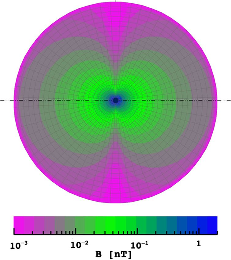
E. FIANDRINI et al.                                                                  PHYS. REV. D 104, 023012 (2021)

during each maximum of solar activity. This periodicity is         In this paper, we present a data-driven analysis of the
important for CR modulation and, in particular, to study the    temporal dependence of the flux of CR protons, which
effects of particle drifts in the large-scale HMF.              constitute the most abundant species of Galactic cosmic
   Since CR modulation is a manifestation of the CR             radiation. The analysis has been conducted using a sto-
propagation through the heliosphere, CR data can be used
                                                                chastic model of CR propagation, i.e., a Monte Carlo–
to investigate the fundamental physics processes governing
                                                                based approach in which the solar modulation effect
the transport of charged particles through the heliospheric
plasma. In particular, precise measurements of the energy       is computed by statistical sampling. Using the recent
                                                                time- and energy-resolved measurements of CR proton
and time dependence of the CR fluxes may help to
                                                                fluxes on BR basis, by means of a procedure of statistical
disentangle the interplay of the different physics mecha-
                                                                inference, we determine the temporal and rigidity depend-
nisms at work. In this respect, the physical understanding of
                                                                encies of the mean free path of CRs propagating through
CR modulation in the heliosphere is one of the main
                                                                the heliosphere, along with the corresponding uncertainties.
objectives of many theoretical and observational studies        The rest of this paper is organized as follows. In Sec. II,
[5–8]. Besides, modeling the CR modulation is essential for     we describe in detail the numerical implementation of the
the search of new physics signatures in the fluxes of CR        CR modulation model, which is based on known and
antimatter such as positrons or antiprotons. An antimatter      conventional mechanisms of particle transport in the helio-
excess in CRs may suggest the occurrence of dark matter         sphere. In Sec. III, we present the procedure for the data-
annihilation processes or the existence of new astrophysical    driven determination of the key model parameters and their
sources of antimatter. Since the low-energy spectra of          uncertainty, which is based on a grid sampling over a
CRs are influenced by solar modulation, any interpretation      multidimensional parameter space. In Sec. IV, we present
about the origin of antiparticles requires an accurate          the fit results and discuss their interpretation, in terms of
modeling of the charge-sign- and energy-dependent effects       physical mechanisms of CR transport, in relation to the
of CR modulation [9]. Understanding the evolution of the        properties of heliospheric environment or with known
CR fluxes in the heliosphere is also important for assessing    proxies of solar activity. We then conclude, in Sec. V,
the radiation hazard to astronauts, electronics, and com-       with a summary of our study and a discussion on its future
munication systems for low-Earth-orbit satellites or deep-      developments.
space missions [10,11]. In fact, the Galactic CR flux
constitutes a significant dose of ionizing radiation for                   II. THE NUMERICAL MODEL
human bodies and electronics, and, thus, an accurate
                                                                   To get a realistic description of CR modulation phe-
knowledge of the temporal and spatial variation of the
                                                                nomenon, one needs to capture the essential features of CR
CR in the heliosphere will reduce the uncertainties in the
                                                                transport in the heliosphere. The diffusive propagation of
radiation dose evaluation [12]. An important challenge,
                                                                the charged particles in the turbulent heliospheric plasma is
in this context, is to establish a predictive model for solar
                                                                described by the Parker equation [18]:
modulation that is able to forecast the CR flux evolution
using solar activity proxies.                                   ∂f                         1               ∂f
                                                                   þ ∇ · ðV⃗ sw − K · ∇fÞ − ð∇ · V⃗ sw Þ         ¼ 0:    ð1Þ
   From the observational point of view, substantial            ∂t                         3             ∂ðln RÞ
progress has been made with the new measurements
                                                                The equation, along with its boundary conditions, describes
of the proton flux from the AMS-02 experiment in the
                                                                the evolution of the distribution function fðt; r⃗ ; RÞ for a
International Space Station [13,14] and the PAMELA
                                                                given particle species, where t is the time and R is the
mission on board the Resurs-DK1 satellite [15,16], along        particle rigidity, i.e., the momentum per charge units
with the data provided by the Voyager-1 spacecraft beyond       R ¼ p=Z. In this paper, we will focus on cosmic protons,
the heliosphere [17]. In particular, AMS-02 and PAMELA          so that R ≡ p. The quantity K is the drift-diffusion tensor
have recently released accurate measurements of CR proton       of the CR particles in the turbulent HMF of the heliosphere.
spectra over Bartels’ rotation (BR) basis (27 days), over an       Because of the complexity of the transport equation,
extended energy range and for extended time periods,            analytical solutions can be found only for very simplified
covering the long solar minimum of 2006–2009 (cycle             situations such as in the force-field or the diffusion-
23=24), the ascending phase of cycle 24, the solar maxi-        convection approximations [19,20]. The full solution
mum and HMF reversal of 2013–2014, and the subsequent           of Eq. (1) can be obtained numerically. Here, we employ
descending phase toward the new minimum until May               the stochastic method that has become widely implemented
2017. Therefore, the data allow for the study of the CR         in recent years thanks to the enormous progress in
propagation in the heliosphere under very different con-        computing speed and resources [8,21,22]. The method
ditions of solar activity and epochs of opposite HMF            consists of transforming the Parker equation into a set of
polarities, which may bring a substantial advance in the        stochastic differential equations (SDEs) and then using
understanding of the solar modulation phenomenon.               Monte Carlo simulations to sample the solution, i.e., the

                                                          023012-2
NUMERICAL MODELING OF COSMIC RAYS IN THE … PHYS. REV. D 104, 023012 (2021)
differential CR intensity for a given species, at a given straight line along the polar axis. Here, we adopt the
position in the heliosphere [23,24]. modification of Jokipii and Kota [28]:
In general, the flux of CRs inside the heliosphere is time 2
dependent, reflecting the varying conditions of the medium r0 2 rδðθÞ 2 1=2
B ¼ B0 1 þ tan ψ þ ; ð3Þ
over which they propagate [25]. A common practice is to r r⊙
follow a quasi-steady-state approximation where the time-
dependent CR modulation is described as a succession of where δðθÞ ¼ 8.7 × 10−5 = sinðθÞ if 1.7° < θ < 178.3° and
steady-state solutions (∂=∂t ¼ 0) and the effective status ≃3 × 10⁻³ otherwise [29]. The winding angle ψ is then
of the heliospheric plasma during the CR propagation is modified as
defined in a suitable way. The approximate way of taking
into account the varying status of the heliosphere during the Ωðr − r⊙ Þ rδðθÞ 2 1=2
tan ψ ¼ þ : ð4Þ
CR propagation is described in Sec. II. Furthermore, in the V r⊙
SDE method, pseudoparticles are propagated backward in The term involving the dimensionless constant δ reflects
time from the Earth position to the heliospheric boundaries. the fact that the random field is equivalent to a small
The numerical engine for handling the Monte Carlo gen- latitudinal component Bθ ∼ δðθÞr=r⊙ . In this way, mod-
eration and the trajectory tracing is extracted from the ifications on HMF and winding angle are effective only
publicly available code SolarProp [21]. Based on the SolarProp near the polar regions, as shown in Fig. 1, where the
simulation framework, we have implemented a customized two quantities are shown as a function of colatitude. It is
model that is described in the following. worth noticing that the definitions of Bθ and δðθÞ imply
∇⃗ ·B⃗ ¼ 0.
A. The modulation region
The heliosphere is a dynamic void in the interstellar 2. Polarity and tilt angle
medium (ISM) generated by the SW and regulated by Sun’s
An important characteristic for the CR solar modulation
activity. The relevant boundary for the CR modulation
is that the HMF follows an ∼22-year cycle, known as the
phenomenon is the heliopause (HP), which separates the
magnetic polarity cycle, characterized by a N/S reversal
heliospheric plasma from the local ISM. The HP is usually
about every ∼11 years, during the maximum of solar
modeled as a spherical structure of radius rHP ≈ 122 AU,
activity. The period when B ⃗ is directed outward in the
where the Sun lies at its center. Within the heliosphere,
the termination shock (TS) is located at rTS ≅ 85 AU, northern hemisphere of the Sun is known as the positive
while the Earth position is at r0 ≡ 1 AU placed in the polarity epoch (A > 0), while when it has the opposite
equatorial plane. direction as the (A < 0) cycle. In practice, the quantity A
is a dichotomous variable that expresses the sign of B-field
projection in the outward direction from the northern
1. The large-scale HMF
The outward-flowing SW embeds a frozen-in HMF,
which is wound up in a modified Parker spiral [26]. The
ideal Parker field is given by
2
⃗B ¼ AB0 r0 ðêr − tan ψ êϕ Þ½1 − 2Hðθ − ΘÞ; ð2Þ
r
where r and θ are the helioradius and colatitude, respec-
tively, B0 is the HMF value at Earth position, A ¼ 1 is
the field polarity, and H is the Heaviside step function.
The winding angle ψ of the field line is defined as
tan ψ ¼ Ωðr − r⊙ Þ sin θ=V sw ; the angle Θ determines the
position of the wavy HCS, given by Θ ¼ π=2 þ
sin−1 ½sin α sin ðΩr=V w Þ [27]. Here, the quantity Ω is the
average equatorial rotation speed ≈2.73 × 10⁻⁶ rad s−1 , α
is the HCS tilt angle, and r⊙ ¼ 696.000 km is the radius of
the Sun. The Parker model overwinds by several degrees
beyond the value of the winding angle ψ, determined by the
model at the polar regions. To avoid this, one has to
consider that solar wind disturbances and plasma waves
propagating along the open field lines modify the magnetic FIG. 1. Side view of the HMF field model in the ðx; zÞ plane of
field at the polar regions, so that it does not degenerate to a the heliosphere. The dashed line is the equatorial plane.
023012-3E. FIANDRINI et al. PHYS. REV. D 104, 023012 (2021)
hemisphere, A ≡ BN =jBN j (or the inward projection of BS
in the southern hemisphere). In practice, it can be deter-
mined using observations of the polar HMF in proximity of
the Sun (Sec. III B). The relevance of magnetic polarity in
the context of solar modulation arises from CR drift
motion: It can be seen (Sec. II B) that the equations ruling
CR drift in the HMF depend upon the sign of the product
between A and q̂ ¼ Q=jQj, where Q is the CR electric
charge. Thus, opposite drift directions are expected for
opposite q̂A conditions. A major corotating structure
relevant to CR modulation is the HCS, which divides
the HMF into hemispheres of opposite (N/S) polarity and
where B ¼ 0. Because of the tilt of the solar magnetic axis,
the HCS is wavy. The level of the HCS waviness changes
with time, and it is set by the tilt angle αðtÞ. Typically, it
varies from α ∼ 5° during solar minimum to α ∼ 70° during
solar maximum. The tilt angle is reconstructed by the
Wilcox Solar Observatory using two different models for
the polar magnetic field: the so-called L model and R
model. In this work, the classical L-model reconstruction is
used as the default.
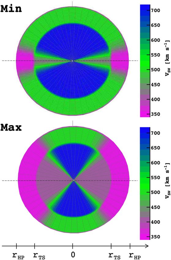
3. The wind
The SW speed V sw is taken as radially directed outward.
However, the wind field exhibits a radial, latitudinal,
and temporal dependence, where the latter is related to
the solar cycle. During periods of solar minimum, the flow
becomes distinctively latitude dependent, changing from
FIG. 2. Side view of the SW speed profile in the ðx; zÞ of the
∼400 km s−1 in the equatorial plane (slow-speed region) to
heliosphere, showing its latitudinal dependence in the typical
∼800 km s−1 in the polar regions (high-speed region), as cases of solar minimum (min, for α ≅ 10°) and solar maximum
observed by Ulysses [30]. This effect is mitigated during (max, for α ≅ 60°), where the latitudinal transition from a slow to
epochs of solar maximum, when the angular extension of a fast region depends on the HCS tilt angle α.
the slow-speed region increases to higher latitudes. Beyond
the TS, the SW slows down by a factor 1=S, where S ¼ 2.5 from the Sun. Beyond the TS, the real SW speed is
is the shock compression ratio, as measured by the Voyager expected to decrease as r−2 , so that ∇⃗ · V⃗ sw ¼ 0 and CR
probes [31]. In this region, the wind is slowed down to particles do not experience adiabatic cooling. The radial
subsonic speed. To incorporate such features in our model, and latitudinal SW profile is shown in Fig. 2 for two values
we adopt the parametric expression given in Ref. [32]: of α corresponding to solar minimum (α ≅ 10°) and solar
maximum (α ≅ 60°) conditions.
V sw ðr; θÞ ¼ V 0 f1.475 ∓ 0.4 tanh ½6.8ðθ − π=2 θT Þg
Sþ1 S−1 r − rTS B. The particle transport
× − tanh ; ð5Þ
2S 2S L The Parker equation for the particle transport contains all
physical processes experienced by a given species of CR
where V 0 ¼ 400 km s−1 and L ¼ 1.2 AU is the scale particles traveling in the interplanetary space. In Eq. (1), the
thickness of the TS. The top and bottom signs correspond drift-diffusion tensor can be written as
to the northern (0 ≤ θ ≤ π=2) and southern hemisphere
(π=2 ≤ θ ≤ π) of the heliosphere, respectively. The angle 2 3
K r⊥ −K A 0
θT determines the polar angle at which the SW speed 6
changes from a slow to a fast region. It is defined as K ¼ 4 KA K θ⊥ 0 75 ð6Þ
θT ¼ α þ δα, where α is the tilt angle of the HCS and 0 0 Kk
δα ¼ 10° is the width of the transition. With this approach,
the angular extension θT of the SW profile changes in time, in a reference system with the third coordinate along the
and it is linked to the level of solar activity, using the angle average magnetic field. The symbol K k denotes the diffusion
α as proxy. The expression is valid for r ≫ r⊙, i.e., away coefficient along the field direction, while K θ⊥ and K r⊥ are
023012-4NUMERICAL MODELING OF COSMIC RAYS IN THE … PHYS. REV. D 104, 023012 (2021)
the diffusion coefficients along the perpendicular and radial for the rigidity and spatial dependence of the parallel
direction, respectively. K A expresses the value of the anti- diffusion coefficient, we adopt a double power-law rigidity
symmetric part of the diffusion tensor, where its explicit dependence and an inverse proportionality with the local
form results from the effects on the motion of CR particles HMF magnitude, following Ref. [32]:
due to drift. V⃗ sw is the SW speed, and V⃗ D is the guiding b−a
center speed for a pitch-angle-averaged nearly isotropic β ðR=R0 Þa ðR=R0 Þh þ ðRk =R0 Þh h
Kk ¼ K0 : ð8Þ
distribution function. The equation can be then rewritten as 3 ðB=B0 Þ 1 þ ðRk =R0 Þh
∂f In this expression, K 0 is a constant of the order of
− ∇ · ½KS · ∇f þ ðV⃗ sw þ V⃗ D Þ · ∇f
∂t 1023 cm2 s−1 , R0 ¼ 1 GV to set the rigidity units, B the
ð∇ · V⃗ sw Þ ∂f HMF magnitude, and B0 the field value at Earth and written
− ¼ 0: ð7Þ in a way such that the units are in K 0 . Here, a and b are
3 ∂ðln RÞ
power indices that determine the slope of the rigidity
The motion of the CR particles in the HMF is usually dependence, respectively, below and above a rigidity Rk,
decomposed in a regular gradient-curvature and HCS drift whereas h determines the smoothness of the transition. The
motion on the background average HMF and a diffusion due perpendicular diffusion in the radial direction is calculated
to the random motion on the small-scale fluctuations of as K ⊥r ¼ ξ⊥r × K k , while the polar perpendicular diffusion
the turbulent HMF. All these effects are included in the was parameterized as K ⊥θ ¼ ξ⊥θ × gðθÞ × K k , where gðθÞ
diffusion tensor K of Eq. (6), which can be decomposed in a is a function that enhances K ⊥θ by a factor d near the poles,
symmetric part that describes the diffusion and an antisym- defined as [32]
metric one that describes the drifts, i.e., K ¼ KS þ KA , with
K Sij ¼ K Sji and K Aij ¼ −K Aji . Particles moving in a magnetic gðθÞ ¼ Aþ ∓ A− tanh ½8ðθA þ π=2 θF Þ: ð9Þ
turbulence are pitch-angle scattered by the random HMF
irregularities. This process is captured by the symmetric Here, A ¼ ðd 1Þ=2, θF ¼ 35°, and θA ¼ θ if θ ≤ π=2 or
θA ¼ π − θ if θ ≥ π=2, with d ¼ 3. The enhancement in the
part of the diffusion tensor KS, which is diagonal if the z
latitude direction of K ⊥θ , together with the anisotropy
coordinate is aligned with the background HMF. Three
between the perpendicular diffusion coefficients and HMF
diffusion coefficients are therefore needed, namely, parallel
modification at the polar regions, is needed to account for
diffusion K k , transverse radial K ⊥r , and transverse polar
the very small latitudinal dependence of the CR intensity, as
diffusion coefficient K ⊥θ . The coefficients can also be it was observed in the Ulysses data [30,40]. The adoption
expressed in terms of mean free path λ along the background of constant ξ⊥ factors implies that K ⊥ and K k follow the
HMF, e.g., K k ¼ βcλk =3 (with β ¼ v=c). The determination
same rigidity dependence, which may be a simplification
of the diffusion coefficients is a key ingredient to study the in the high-R domain [36,41]. Nonetheless, QLT-based
propagation of charged particles in turbulent magnetic fields simulations agree for nearly rigidity-independent ξ, with
like the HMF and is the subject of many theoretical and the typical value of 0.02–0.04 [34,42]. In this work, the
computational studies. The quasilinear theory (QLT) has parameters ξ⊥r and ξ⊥θ are fixed to the value 0.02. We now
been successful at describing parallel diffusion, especially in turn on drift effects, that account for the charge-sign and
its time-dependent and nonlinear extensions [33]. Regarding polarity dependence of CR transport in the HMF [27,43].
perpendicular diffusion, the QLT provides upper limits The regular motion of CRs on the large-scale HMF is
within the field line random walk description [33,34], given by the pitch-angle-averaged guiding center drift
while the best approaches follow the nonlinear guiding
speed hV⃗ D i. It can be related to the antisymmetric part
center theory [35–37].
of the diffusion tensor [44]:
From a microscopic point of view, CR diffusion is linked
to the resonant scattering of particles with rigidity R with ∂K Aij
the HMF irregularities around the wave number kres ∼ hðV D Þi i ¼ ; ð10Þ
∂xj
2π=rL , where rL ¼ R=B. The essential dependence of λk
on the HMF power spectrum can be expressed as where the antisymmetric part of the tensor has the form
λk ∼ r2L hB2 i=wðkres Þ ∼ R2 =wðkres Þ, where hB2 i is the mean
Bk
square value of the background field and wðkres Þ is the K Aij ¼ K A uðθÞζðRÞϵijk : ð11Þ
power spectrum of the random fluctuations of the HMF B
around the resonant wave number. The power spectral Here, ϵijk is the Levi-Civita symbol, uðθÞ is a function that
density follows a power law as wðkÞ ∼ k−ν , where the index describes the transition between the region influenced by
ν depends on the type and on the spatial scales of the the HCS and the regions outside of it, and ζðRÞ is a function
turbulence energy cascade [38,39]. Therefore, λk depends of rigidity that suppresses drifts at low rigidity. To deter-
on the turbulence spectral index as λk ∼ R2−ν . In this work, mine the value of K A , we note that the small value of the
023012-5E. FIANDRINI et al. PHYS. REV. D 104, 023012 (2021)
ratio K ⊥ =K k suggests that CR particles move over many where the reduction occurs at rigidity below the cutoff
gyro-orbits in a mean free path; therefore, the drift motion value RA ¼ λ⊥ δBT , which depends on the perpendicular
is weakly affected by scattering. In the weak scattering diffusion length and total variance of the HMF. The
approximation, one has reduction is effective at R ≪ RA , when ζ ≈ ðR=RA Þ2 ≪ 1,
while in the high-R limit one has ζ ≈ 1. The cutoff value RA
Q βR depends on the HMF turbulence through λ⊥ and δBT .
K A ¼ K 0A ; ð12Þ
jQj 3B With typical values of λ⊥ ≈ 1.5 × 10⁻³ AU and δBT ≈
3.5 nT for the considered epochs, one can estimate
where Q is the CR particle charge and K 0A is a normali-
RA ≈ 0.3–0.6 GV. In this work, we have fixed it at
zation factor ≤ 1. Drift motion is relevant close the HCS, 0.5 GV, corresponding to a proton kinetic energy of
where CRs cross many times regions of opposite HMF
125 MeV. The normalization K 0A factor is fixed to 1, so
polarity. A 2D description of HCS drift is given in Burger
that the whole drift reduction is regulated by ζ.
and Hattingh [44]. In this approach, the drift velocity is
The most relevant feature of magnetic drift is that its
given by
direction depends on the sign of the charge, q̂ ¼ Q=jQj,
⃗ þ H;
hV⃗ D i ¼ ζðRÞ½G ⃗ ð13Þ and on the HMF polarity A, via the product q̂A, so that
particles with opposite q̂A will drift in opposite directions
where the two vectors are defined as follows: and will follow different trajectories in the heliosphere.
This characteristic is expected to give observable charge-
⃗
B sign dependence in the CR modulation. Finally, in a
G ⃗ ¼ uðθÞ∇ × K A ;
B reference frame with the z coordinate along the average
magnetic field, the diffusion tensor is given by Eq. (6).
⃗
H⃗ ¼ ∂uðθÞ K A e⃗ θ × B : ð14Þ The effective diffusion tensor in heliocentric polar
∂θ r B coordinates is obtained by a coordinate transformation
in the modified Parker field. In our 2D approach, the
The G ⃗ term in Eq. (14) describes the gradient-curvature
relevant components are K rr ¼ K k cos2 ψ þ K ⊥r sin2 ψ,
⃗ term describes the particle motion across the
drifts, the H K θθ ¼ K ⊥θ , and K θr ¼ K A sin ψ ¼ −K rθ .
region affected by the HCS, e⃗ θ is the unit vector along the
polar direction, and uðθ) is given by
C. The proton LIS
ð1=ah Þ arctanf½1 − ð2θ=πÞ tan ah g if ch < π=2; To resolve the modulation equation for cosmic protons,
uðθÞ ¼
1 − 2Hðθ − π=2Þ if ch ¼ π=2 their LIS must be specified as a boundary condition. The
determination of the CR proton LIS requires a dedicated
ð15Þ modeling effort, starting from the distribution of Galactic
CR sources and accounting for all the relevant physical
with H the Heaviside step function,
processes that occur in the interstellar medium. In this
work, we adopt an input LIS for CR protons that relies on a
π
ah ¼ arccos −1 ; ð16Þ two-halo model of CR propagation in the Galaxy [47,48].
2ch
In this model, the injection of primary CRs in the ISM
and is described by rigidity-dependent source terms S ∝
ðR=GVÞ−γ with γ ¼ 2.28 0.12 for protons. The diffusive
π 1 2rL transport in the L-sized Galactic halo is described by
ch ¼ − sin α þ : ð17Þ
2 2 r an effective diffusion coefficient D ¼ βD0 ðR=GVÞδi=o with
D0 =L ¼ 0.01 0.002 kpc=Myr [9,48]. The two spectral
The angle 2rL =r depends on the maximum distance that a indices δi=o describe two different diffusion regimes in the
particle can be away from the HCS while drifting. Finally,
inner and outer halo, with δi ¼ 0.18 0.05 for jzj < ξL
the function uðθÞ is such that uðπ=2Þ ¼ 0, uðch Þ ¼ 0.5, and
(inner halo) and δo ¼ δi þ Δ for jzj > ξL (outer halo), with
∂uðπ=2Þ=∂θ ¼ 1. CR drift coefficients are expected to be
Δ ¼ 0.55 0.11. The z variable here is the vertical spatial
reduced in the presence of turbulence as results theoreti-
coordinate. The half thickness of the halo is L ≅ 5 kpc, and
cally and from numerical test-particle simulations [45,46].
the near-disk region (inner halo) is set by ξ ¼ 0.12 0.03.
In this work, we use a simple approach to incorporate drift
Finally, we considered the impact of diffusive reaccelera-
reduction. Following Ref. [46], we adopt a reduction factor
of the type tion. Within the two-halo model, the interstellar Alfvénic
speed is constrained from the data to lie between 0 and
1 6 km s−1 . Calculations of the proton LIS were constrained
ζ¼ R2
; ð18Þ by various sets of measurements: low-energy proton data
1 þ RA2 (at 140–320 MeV) collected by Voyager-1 beyond the HP
023012-6NUMERICAL MODELING OF COSMIC RAYS IN THE … PHYS. REV. D 104, 023012 (2021)
mathematical framework described Sec. II. In practice,
we defined a set of physics observables, to be computed as
model predictions, and a set of model parameters, to be
determined by statistical inference.
A. The cosmic ray data
The data used in this work consist in time-resolved
and energy-resolved measurements of CR proton fluxes,
in the kinetic energy range from ∼80 MeV to ∼60 GeV.
Specifically, we use the 79 BR-averaged fluxes measured
by the AMS-02 experiment in the International Space
Station from May 2011 to May 2017 [13] and the 47 þ 36
BR-averaged fluxes observed by the PAMELA instrument
in the satellite Resurs-DK1 from June 2006 to January 2014
[15,16]. The data sample corresponds to a total of 10 101
FIG. 3. Proton LIS used as input boundary condition for
data points collected over a time range of about 11 years,
the modulation along with the estimated uncertainty band from the solar minimum from 2006 to 2009, the ascending
[47–49,53]. Data from Voyager-1 in interstellar space and from phase to solar maximum, when the HMF polarity A
AMS-02 and PAMELA in low Earth orbit collected during two reversed from A < 0 to A > 0, and the following descend-
epochs. ing phase until May 2017. These data have been retrieved
by the ASI-SSDC cosmic ray database [54].
The intensity of the CR proton fluxes in the energy range
and high-energy proton measurements (E ≳ 60 GeV) made between 0.49 and 0.62 GeV are shown in Fig. 4 as a
by AMS-02 in low Earth orbit, along with measurements of function of time for both the PAMELA and AMS-02
the B/C ratio from both experiments. The latter were datasets. From the figure, the complementarity of the
essential to constrain the diffusion parameters of the LIS two experiments is apparent. It can be seen that the highest
model [9]. Details on this model are provided elsewhere intensity of the CR is reached during ∼ December 2009,
[48,49]. The resulting proton LIS is shown in Fig. 3 in i.e., under the solar minimum, while the lowest intensity
comparison with the data from Voyager-1, along with occurs in ∼ February 2014, around solar maximum. The
PAMELA and AMS-02 measurements made in March vertical dashed line of the figure shows the HMF reversal
2009 and April 2014, respectively. The uncertainty band epoch T rev , along with the transition region shown as a
associated with the calculations is also shown in the figure. shaded area where the HMF is disorganized and the
This model is in good agreement with other recently polarity is not defined. The determination of T rev and
proposed LIS models [5,22,50–52]. the transition region are presented later on.
III. DATA ANALYSIS B. The parameters
In this section, we present the analysis method by which The numerical model presented in Sec. II makes use of
we extract knowledge and insights from the data using the several physics input to be determined with the help of
FIG. 4. BR-averaged flux J 0 evaluated in the reference energy range between 0.49 and 0.62 GeV from PAMELA (open squares)
[15,16] and AMS-02 (filled circles) [13,14]. The vertical dashed line shows the epoch of the HMF polarity inversion, along with the
shaded area indicating the reversal epoch.
023012-7E. FIANDRINI et al. PHYS. REV. D 104, 023012 (2021)
observations. Inputs include solar parameters, character- A similar estimate is done for the polar magnetic field and
izing the conditions of the Sun or the interplanetary plasma, for the resulting polarity Â, in Fig. 5(d). The latter can be
and transport parameters that describe the physical mech- regarded as a “smoothed” definition for the magnetic
anisms of CR propagation through the plasma. Solar and polarity A, otherwise dichotomous (A ¼ 1). When the
transport parameters are interconnected with each other, HMF is in a defined polarity state, one has  ¼ 1. During
and they may show temporal variations related to the solar the HMF reversal transition epoch (shaded area in the
cycle. For instance, solar parameters such the magnetic figures), as the polarity is not well defined, the estimate of
field magnitude, its variance, and its polarity are trans- Â takes a floating value between −1 and þ1.
ported from the Sun into the outer heliosphere, therefore At this point, we also recall that several parameters
provoking time-dependent CR diffusion and drift. entering the model that have been kept constant in the
We identified, in our model, a set of six time-dependent simulation, i.e., assumed to be known or time independent.
key parameters that are of relevance for the phenomenology The HP and TS positions were fixed at rHP ¼ 122 AU and
of CR modulation. They are the tilt angle of the HCS αðtÞ, rTS ¼ 85 AU, respectively, deduced from the Voyager-1
the strength of the HMF at the Earth location B0 ðtÞ, the observations. The data suggest that the TS may vary over
HMF polarity AðtÞ, and the three diffusion parameters the solar cycle of the order of a few AU, but its impact in the
appearing in Eq. (8): the normalization factor of the parallel CR fluxes is not negligible [51].
diffusion tensor, K 0 ðtÞ, and the two spectral indices of the The h parameter of Eq. (8), describing the smoothness of
rigidity dependence of CR diffusion, aðtÞ and bðtÞ, below the transition between the two diffusion regimes below and
and above the break Rk , respectively, as seen in Eq. (8). above Rk , was kept constant at h ¼ 3. Within the precision
Note that all key parameters are expressed as continuous of the data, the h parameter has no appreciable impact on
functions of time t, but, in practice, they have been the CR fluxes. Similarly, the rigidity break Rk for K k was
determined for the epochs corresponding to the CR flux
kept fixed at the value 3 GV. This parameter represents the
measurements.
scale rigidity value where the CR Larmor radius matches
The three solar parameters α, B0 , and A can be
the correlation length of the HMF power spectrum, which is
determined from solar observatories: Data of HMF polarity
at the GV scale. Regarding the value of Rk , we found that
and tilt are provided by the Wilcox Solar Observatory on
time variations on this quantity do not give appreciable
10-day or BR basis. Measurements of the HMF B0 at 1 AU
variations in the CR fluxes (see, e.g., Ref. [32]). The ξ⊥i
are done in situ on a daily basis, since 1997, by the
coefficients for the diffusion tensor, for the values used
Advanced Composition Explorer (ACE) on a Lissajous
here, represent a widely used assumption (e.g., Ref. [40]).
orbit around L1 [55]. It is important to notice that, in this
The polar enhancement factor of Eq. (9) is kept constant at
study, our aim is to capture the effective status of the large- d ¼ 3 for ξ⊥θ so that the condition K ⊥ =K k ≪ 1 is still
scale heliosphere sampled by CRs detected at a given
fulfilled at the polar regions. Regarding magnetic drift, the
epoch t, and this is connected to solar-activity parameters
critical rigidity RA of Eq. (18) is kept constant at 0.5 GV
that are precedent to that epoch. In fact, several studies have
following previous studies and independent observations
reported a time lag of a few months between the solar
on the CR latitudinal gradient [32,57]. This choice could
activity and the varying CR fluxes [51,56], reflecting the
be tested only with low-rigidity CR data (R ≪ RA ), as our
fact that the perturbations induced by the Sun’s magnetic
results are insensitive to the exact value of RA . The
activity take a finite amount of time to establish their effect
in the heliosphere. To tackle this issue, for each epoch t normalization factor for drifts speeds K 0A was chosen to
associated to a given CR flux measurement, we perform a be unity such to set “full drift” speeds in the propagation
backward-moving average (BMA) for α and B0 , and A, i.e., model for all the periods, and this drift reduction is entirely
a time average of these quantities calculated over a time given by Eq. (18). Reductions in the K 0A value may occur
window[t − τ, t]. The window extent τ is the time needed during periods of strong magnetic turbulence, e.g., during
by the SW plasma to transport the magnetic perturbations solar maximum [25,57].
from the Sun to the HP boundary, which ranges between ∼8
(fast SW speed) and ∼16 months (slow SW speed). In the C. The statistical inference
case of α, the window is large, because the HCS is always
mostly confined in the slow (equatorial) SW region. In the 1. The parameter grid
case of B0 , the BMA has to be computed by an integration The transport parameters K 0 ðtÞ, aðtÞ, and bðtÞ have
over the latitudinal profile of the SW speed at a given been determined from the AMS-02 and PAMELA data by
epoch. Our estimations are consistent with the lag reported means of a global fitting procedure. For this purpose, a six-
in other studies [51,56] and supported by correlative dimensional discrete grid of the model parameter vector
analysis that we made a posteriori. Figure 5 shows the q⃗ ¼ (α, B0 , A, K 0 , a, b) was built; i.e., the model was run
reference parameters B̂0 and α̂ calculated for each reference for every node of the grid such as to produce a theoretical
epoch t corresponding to a BR-averaged CR measurement. calculation for the CR proton flux. In the grid, the
023012-8NUMERICAL MODELING OF COSMIC RAYS IN THE … PHYS. REV. D 104, 023012 (2021)
(a)
(b)
(c)
FIG. 5. Reconstruction of the tilt angle α, the local HMF strength B0 , and the magnetic polarity A as a function of the epoch, evaluated
with the BMA procedure in correspondence of the epochs of the PAMELA and AMS-02 flux measurements. The vertical dashed line
marks the HMF reversal T rev . The shaded area around T rev represents the effective period of the HMF polarity transition. The raw data,
shown as thin shaded lines, are taken from the ACE space probe and from the Wilcox Solar Observatory [4,55].
parameter α ranges from 5° to 75° with steps of 10° and B0 Jd ðE; tÞ, representing a set flux measurements as a
from 3 to 8 nT with steps of 1 nT, and the polarity A takes function of energy for a given epoch t, a χ 2 estimator
the two values A ¼ þ1 and A ¼ −1. The parameter K 0 was evaluated as
ranges from 0.16 to 1.5 × 1023 cm2 s−1 , with steps of
0.08 × 1023 cm2 s−1 , and the indices a and b range from X ½Jd ðEi ; tÞ − Jm ðEi ; q⃗ Þ2
0.45 to 1.65 with steps of 0.05. The total number of grid χ 2 ð⃗qÞ ¼ : ð19Þ
i
σ 2 ðEi ; tÞ
nodes amounts to 938 400. For each node of the parameter
grid, a theoretical prediction for the modulated proton flux
Jm ðE; q⃗ Þ was evaluated, as a function of kinetic energy, Similarly to J m , the χ 2 estimator is built such as to be a
over 120 energy bins ranging from 20 MeV to 200 GeV continuous function of the parameters q⃗ , except for the
with log-uniform steps. Using the SDE technique, 2 × 10³ variable A that is treated as discrete. From the χ 2 estimator,
pseudoparticles were Monte Carlo generated and retro- the transport parameters fK 0 ; a; bg can be determined by
propagated for each energy bin. This task required the minimization at any epoch, while the solar parameters
simulation of about 14 billion trajectories of pseudopro- fB0 ; α; Ag can be considered as “fixed inputs,” as they are
tons, corresponding to several months of CPU time. Once determined by the epoch t using the BMA reconstruction
the full grid was completed, the output flux was tabulated presented above. For a given set of BMA inputs such as B̂0
and properly interfaced with the data. For each dataset and α̂, the flux Jm ðE; q⃗ Þ can be expressed as a continuous
023012-9E. FIANDRINI et al. PHYS. REV. D 104, 023012 (2021)
function of the parameters by means of a multilinear
interpolation over the grid nodes. In the α − B0 plane,
one has αj < α̂ðtÞ < αjþ1 and B0k < B̂0 ðtÞ < B0;kþ1 , where
αj and B0;k are the closest values of the grid corresponding
to their BMA averages. Regarding polarity A, both 1
evaluations were done under the assumption that the
polarity is known. The flux model dependence upon energy
should also be handled. In Eq. (19), Ei are the mean
measured energies reported from the experiments (coming
from binned histograms). In general, the Ei array does not
correspond to the energy grid of the model. The model
evaluation of Jm ðE; q⃗ Þ at the energy Ei was done by log-
linear interpolation.
2. The uncertainties
The σ factors appearing in Eq. (19) represent the total
FIG. 6. Error band reflecting the statistical uncertainty of the
uncertainties associated with the flux. They can be written Monte Carlo–generated trajectories. Low-energy CRs have less
as σ 2 ðEi ; tÞ ¼ σ 2d ðEi ; tÞ þ σ 2m ðEi ; tÞ. Here, σ 2d ðEi ; tÞ are the chance to reach the inner heliosphere, giving a higher uncertainty
experimental errors associated to the flux measurement on the Monte Carlo statistics.
of the ith energy bin around Ei , while σ 2m ðEi ; tÞ are the
theoretical uncertainties of the flux calculations evaluated
estimated that the uncertainty introduced by the interpola-
at the same value of energy. Uncertainties in experimental
tion, rather than the direct simulation with of Jð⃗q; EÞ, is
data are of the order of 10% in the PAMELA data and ∼2%
always of the order of 1%. An important source of
in the AMS-02 data, although they depend on kinetic
systematic error is the uncertainty coming from the input
energy. Theoretical uncertainties include statistical fluctu-
LIS of CR protons; see Sec. II C. The LIS uncertainties are
ations of the finite SDE generation of pseudoparticle
highly energy dependent. They are significant in the energy
trajectories. Uncertainties are relevant at low energy where,
region of ∼1–10 GeV (up to 30% and more), where direct
due to the heavy adiabatic energy losses, the Monte Carlo
interstellar data are not available but the modulation effect
sampling suffers from a smaller statistics. Thus, after
is still considerable. However, in this energy region, the
repeating many times the simulation with the same modu-
Galactic transport parameters regulating the LIS intensity
lation parameters, the modulated flux will fluctuate around
are in degeneracy with the free parameters of CR diffusion
an average value because of the random process of
(Sec. III B) and, in particular, with K 0 [49]. Such a
pseudoparticle propagation with the SDE approach.
degeneracy translates into a correlation between the best-
These fluctuations can be arbitrarily reduced with the
fit K 0 values and the LIS intensity at the GeV scale which,
increase of the pseudoparticle generation, but at the
in turn, determines the absolute scale of the modulated CR
expense of a large CPU time. The evaluation of these
flux J0 at the GeV scale. The K 0 − J0 correlation is also
uncertainties can be done as follows. Given N m as the
discussed in Sec. IVA. To estimate the impact of the LIS
number of pseudoparticles that reach the boundary with
uncertainty on the temporal dependence of the best-fit
energy E, and N G as the number of pseudoparticles
parameters of CR diffusion in the heliosphere, we pro-
generated at the same energy, the ratio of the modulated
ceeded as in Refs. [49,53]. We performed dedicated runs of
flux to the LIS flux is Jm =JLIS ≈ N m =N G . Since the
fitting procedure for a large number of randomly generated
propagation process is stochastic in nature, the relative pffiffiffiffiffiffiffi LIS functions where, for each input LIS, the time series
error of the modulated flux scales as δJm =Jm ¼ 1= N m , of the diffusion parameters were determined. In practice,
where N m ¼ N G ðJm =JLIS Þ. We found that the generation of the LIS functions were generated using the Monte Carlo
N ≅ 2 × 10³ pseudoparticles for each energy bin is suffi- framework in Ref. [48], i.e., according to the probability
cient for being not dominated by SDE-related uncertainties. density function of the Galactic CR transport parameters.
The relative uncertainties as a function of kinetic energy are With this procedure, the systematic uncertainties associated
shown in Fig. 6. The errors are about ∼10%–20% at with the LIS modeling are included in the final errors with a
20 MeV of energy and decrease with increasing energy. proper account for their correlations.
They become constant at ∼2% above a few GeV. A minor
source of systematic error comes from the multilinear
interpolation of the parameter and energy grid, i.e., from 3. The reversal phase
the method we used to evaluate the flux at any arbitrary set The parameter T rev marks the epoch of the 2013 magnetic
of parameters and energy. From dedicated runs, we have reversal, where the HMF flipped from negative to positive
023012-10NUMERICAL MODELING OF COSMIC RAYS IN THE … PHYS. REV. D 104, 023012 (2021)
polarity states. The polarity of the HMF, however, is well 4. The parameter extraction
defined only for t ≪ T rev and t ≫ T rev , where the large- Our determination of the diffusion parameters K 0 ðtÞ,
scale HMF structure follows a dipole-like Parker field to a aðtÞ, and bðtÞ is based on the least squares method. In
good approximation. During reversal, the polarity of the practice, we proceeded as follows. Given a set of CR proton
field is less sharply defined, and the HMF field follows a flux measurements Jd ðE; tÞ, for each parameter x ¼ K 0 ðtÞ,
more complex dynamic (e.g., Ref. [58]). A way to account aðtÞ, and bðtÞ, the corresponding χ 2 ðxÞ distribution,
for this situation is to use a generalized definition of defined as in Eq. (19), is evaluated. The evaluation is done
polarity, such as the BMA reconstruction  in Fig. 5 which for all values of the other parameters y ≠ x, marginalized
ranges from −1 to þ1. For any given parameter configu- over the hidden dimensions. This returns a curve χ 2min ðxÞ as
ration q, the flux model J m ðE; q⃗ Þ can be built as a linear a function of the parameter x and minimized over all hidden
combination of fluxes with defined polarities, weighted by dimensions. From the minimization of χ 2min ðxÞ, the best-fit
a transition function P ≡ ð1 − ÂÞ=2: parameter x̂ and its corresponding uncertainty are esti-
mated. For the minimization, we tested two approaches.
J m ðE; q⃗ Þ ¼ J −m ðE; q⃗ − ÞP þ Jþ ⃗ þ Þ½1 − P;
m ðE; q ð20Þ One method consisted in the interpolation with a cubic
spline of the whole χ 2min ðxÞ curve. A second method, similar
where q⃗ ðÞ ¼ fα; B0 ; A ; K 0 ; a; bg is a vector of parame- to Corti et al. [5], consisted in the determination of
ðÞ
ters with fixed polarity A ¼ 1 and Jm are the corre- the minimum xi;min point from a parameter scan over the
sponding modulated fluxes. The weight P ranges from grid and then by making a parabolic refitting of the χ 2min ðxÞ
1 to 0, for floating polarity  ranging from −1 to 1. The curve around the xi;min and its adjacent points. The position
time dependence of the PðtÞ function associated to the of the minimum and its uncertainty can be calculated as
polarity ÂðtÞ in Fig. 5 can be expressed as follows: estimation of xbest . The errors on the parameters are
estimated as σ x ¼ maxðjx− − xbest j;jxþ − xbest jÞ, where x
PðtÞ ¼ ½1 þ eðt−T rev Þ=δT −1 ; ð21Þ is the parameter value such that χ 2min ðx Þ ¼ χ 2min ðxbest Þ þ 1
above and below xbest, which is the standard error estima-
where δT ≅ 3 months. The transition function PðtÞ is such tion of the least squares method. The little discrepancy of
that P ≅ 0 (P ≅ 1) for t ≲ 3T rev (t ≳ 3T rev ) within 1% level the two methods was used as a systematic error which,
of precision; i.e., when t ¼ T rev 3δT, the flux is 99% however, turned out to be negligible in comparison with the
made of a fixed polarity, while the maximum mixing is for standard errors of the fit. The shapes of the χ 2min projections
t ¼ T rev when PðtÞ ¼ 1=2. It is worth noticing that Eq. (20) as a function of the diffusion parameters is illustrated in
relies on the implicit assumption that, during HMF reversal, Fig. 7 for two distinct epochs, March 2009 (BR 2379,
the modulated flux of CRs can be regarded as a super- during solar minimum) and April 2014 (BR 2466, during
position of fluxes with positive and negative polarity states. solar maximum). For each curve, the best-fit parameter x̂ is
We also note that this approach enabled us to define the shown (vertical line) along with its associated uncertainty
transition epoch, from a smoothed definition of the polarity σ x (shaded band). In the two considered epochs, the data
Â, which is indicated by the shaded area in Fig. 5. Such a come from PAMELA and AMS-02 experiments, respec-
definition of the transition epoch is consistent with esti- tively. As seen from the figure, AMS-02 gives, in general,
mations of the reversal epoch based on the dynamics of the large χ 2 values in comparison with PAMELA. In both time
HMF topology [58,59]. series, the convergence of the fit is good and the parameters
FIG. 7. One-dimensional projections of the χ 2 surfaces as a function of the transport parameters K 0 , a, and b evaluated for two epochs:
March 2009 (pink dashed line) and April 2014 (green continuous line). In the two epochs, representing solar minimum and solar
maximum conditions, the CR flux data come from PAMELA and AMS-02, respectively.
023012-11E. FIANDRINI et al. PHYS. REV. D 104, 023012 (2021)
FIG. 8. Example of multilinear flux interpolation. The thick
FIG. 9. Best-fit fluxes for selected datasets corresponding to
long-dashed line represents the interpolated best flux fit to the
PAMELA (dotted lines) and AMS-02 (solid lines) measurements.
dataset for BR 2435, December 2011. The colored curves
The long-dashed line represents the proton LIS used in this work.
show the 32 fluxes corresponding to the array models such that
xi ≤ xbest < xiþ1 (where x ¼ α, B0 , K 0 , a, and b) used for the
interpolation. A. Temporal dependencies
The main results on the parameter determination pro-
are well constrained. It can be seen that the AMS-02 data cedure are illustrated in Fig. 10. The figure shows the best-
provide tight constraints on the K 0 and b parameters, while fit model parameters K 0 , a, and b as a function of the epoch
the parameter a is more sensitive to low-rigidity data and, corresponding to the measurements of AMS-02 (filled
thus, it is better constrained by PAMELA. After the best-fit circles) and PAMELA (open squares). The vertical dashed
parameters have been determined for a give set of data, the line and the shaded area around it represent the reversal
best model flux Jbest ðEÞ is recalculated using a multilinear phase, as in the previous figures. As a proxy for solar
interpolation over the five-dimensional grid such that activity, Fig. 10(d) shows the monthly SSN data. The solid
xi ≤ xbest < xiþ1 , where x ¼ α, B0 , K 0 , a, and b. In this line shows the smoothed SSN values, obtained with a
procedure, the polarity A is not involved, because it is moving average within a time window of 13 months, along
regarded as a fixed parameter. The flux determination done with its uncertainty band. It can be seen that the diffusion
under both Aþ and A− hypotheses gives the two J fluxes parameters show a remarkable temporal dependence, and
of Eq. (20). The best model is shown in Fig. 8 as a thick such a dependence is well correlated with solar activity.
long-dashed line, along with 32 flux calculations of all From the figure, it can be seen that the normalization of the
adjacent grid nodes. The model is superimposed to the data parallel diffusion coefficient K 0 shows a clear temporal
from PAMELA corresponding to December 2011 (BR dependence. The diffusion normalization appears to be
2445). During this epoch, the HMF was in well-defined maximum in the A < 0 epoch before reversal (t ≪ T rev )
negative polarity state. All fluxes in the figure are calcu- and, in particular, during the unusually long solar minimum
lated for A ¼ −1, i.e., with P ¼ 1. of 2009–2010. The minimum of K 0 is reached during solar
maximum in 2014, about one year after polarity reversal.
From the comparison between Figs. 10(a) and 10(d), the K 0
IV. RESULTS AND DISCUSSION
parameter appears anticorrelated with the monthly SSN.
Here, we present the results of the fitting procedure Physically, larger values of K 0 imply faster CR diffusion
described in Sec. III C and implemented using the consid- inside the heliosphere, thereby causing a milder attenuation
ered dataset on CR protons of Sec. III A. We found that the of the LIS, i.e., giving a higher flux of cosmic protons in the
agreement between best-fit model and the measurements on GeV energy region. In contrast, lower K 0 values imply
the fluxes of CR protons was, in general, very good for all slower CR diffusion, which is typical in epochs of high
the datasets and over the whole rigidity range. In Fig. 9, the solar activity where the modulation effect is significant.
best-fit models for the proton fluxes are shown as colored Qualitatively, this behavior can be interpreted within the
lines for some selected epochs, along with the CR proton force-field approximation where, in fact, positive correla-
LIS. The calculations are compared with the data from tion is expected between SSN and the modulation potential
experiments PAMELA and AMS-02 at the corresponding ϕ ∝ 1=K 0 [9]. Within the framework of the force-field
epochs. The long-dashed line represents the proton LIS model, the parameter ϕ is interpreted as the average kinetic
model used in this work and presented in Sec. II C. energy loss of CR protons inside the heliosphere.
023012-12You can also read