A Comparison of Local Path Planning Techniques of Autonomous Surface Vehicles for Monitoring Applications: The Ypacarai Lake Case-study - MDPI
←
→
Page content transcription
If your browser does not render page correctly, please read the page content below
sensors
Article
A Comparison of Local Path Planning Techniques of
Autonomous Surface Vehicles for Monitoring
Applications: The Ypacarai Lake Case-study
Federico Peralta 1 , Mario Arzamendia 1 , Derlis Gregor 1 , Daniel G. Reina 2            and
Sergio Toral 2, *
 1    Facultad de Ingeniería, Universidad Nacional de Asunción, 2160 San Lorenzo, Paraguay;
      fperalta@ing.una.py (F.P.); marzamendia@ing.una.py (M.A.); dgregor@ing.una.py (D.G.)
 2    Universidad de Sevilla, 41004 Sevilla, Espana; dgutierrezreina@us.es
 *    Correspondence: storal@us.es

 Received: 23 January 2020; Accepted: 7 March 2020; Published: 9 March 2020

 Abstract: Local path planning is important in the development of autonomous vehicles since it
 allows a vehicle to adapt their movements to dynamic environments, for instance, when obstacles are
 detected. This work presents an evaluation of the performance of different local path planning
 techniques for an Autonomous Surface Vehicle, using a custom-made simulator based on the
 open-source Robotarium framework. The conducted simulations allow to verify, compare and
 visualize the solutions of the different techniques. The selected techniques for evaluation include A*,
 Potential Fields (PF), Rapidly-Exploring Random Trees* (RRT*) and variations of the Fast Marching
 Method (FMM), along with a proposed new method called Updating the Fast Marching Square
 method (uFMS). The evaluation proposed in this work includes ways to summarize time and
 safety measures for local path planning techniques. The results in a Lake environment present the
 advantages and disadvantages of using each technique. The proposed uFMS and A* have been
 shown to achieve interesting performance in terms of processing time, distance travelled and security
 levels. Furthermore, the proposed uFMS algorithm is capable of generating smoother routes.

 Keywords: autonomous surface vehicle; local path planning; monitoring applications; motion
 planning; Ypacarai lake

1. Introduction
     Nowadays numerous applications including data collecting, intelligent transport systems,
monitoring of water masses, disaster relief and surveillance, among others, are accomplished by
the use of unmanned vehicles, both aerial and/or aquatic vehicles [1]. Unmanned vehicles present
important advantages, such as low cost in terms of hardware since they usually have smaller
dimensions compared with classical vehicles, and also, they do not need personnel on board since
they are self-managed. However, they do require an increase of complexity for the control system.
Depending on the environment where they operate in, they can be classified as aerial, underwater,
surface or ground vehicles, normally abbreviated as Autonomous Aerial Vehicles (AAV), Autonomous
Underwater Vehicle (AUV), Autonomous Surface Vehicle (ASV) and Autonomous Ground Vehicle
(AGV) respectively [2]. This work is focused on ASV, which are used in water masses like rivers, lakes
and seas for monitoring tasks [3], such as surveillance [4] and bathymetry [5]. When multiple vehicles
cooperate each other, they can form swarms, working in a centralized or distributed way to accomplish
a target mission efficiently [6]. Furthermore, they can act as a communication repeater or extender in a
network of autonomous vehicles [7].

Sensors 2020, 20, 1488; doi:10.3390/s20051488                                  www.mdpi.com/journal/sensors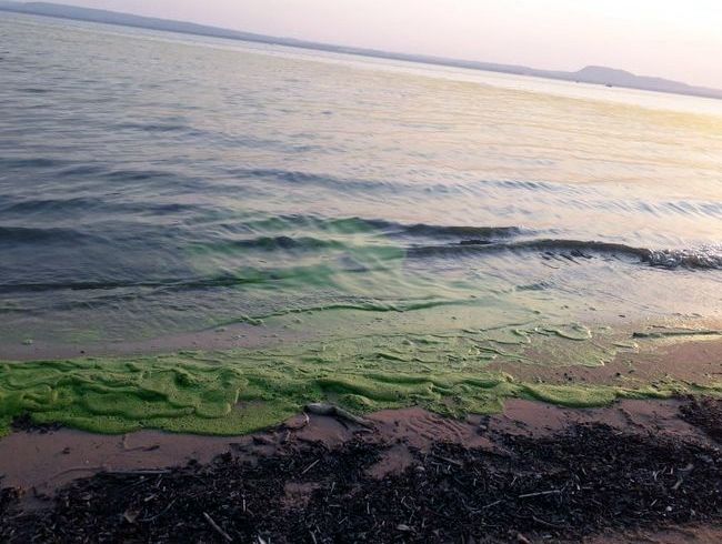
Sensors 2020, 20, 1488                                                                              2 of 28

      For the development of ASVs, several aspects need to be taken into account; according
to [1], the most important features include the control model, the vehicle characteristics and
navigation/guidance systems. The latter refers to both localization of the vehicle within the
environment and motion planning, which are techniques implemented to plan ahead road maps
to accomplish a maneuver or movement goal. While these systems work closely together, methods
and techniques are not similar. Although this work focuses on motion planning techniques, it is worth
mentioning some localization techniques, which in general are crucial in real-life scenarios, as the ones
described in [8], which carefully characterizes the error of the position estimation of an AGV using
three different methods, using as ground truth a robotic total station: odometry, extended Kalman
filters ([9]) and ultra-wideband localization systems. In respect to motion path planning approaches for
ASV, in [10] these techniques have been classified in different levels. At first level, the techniques are
divided into global (offline) path planning and local (online) path planning techniques [11]. In global
path planning approaches, which are proactive, an initial path is calculated with the available global
map information to reduce a target metric like the travelled distance by the vehicle [12]. For instance,
calculating the path planning as a sequence of waypoints to visit. On the other hand, the local path
planning techniques are reactive approaches, which are used to adapt the initial path calculated by the
global planner to unforeseen situations like the appearance of obstacles. Therefore, both techniques can
be considered complementary and should be used in the implementation of path planning approaches
in real ASV applications.
      This work compares several local path planning approaches for monitoring application of the
Ypacarai Lake in Paraguay. This lake is known to contain a high concentration of phosphor and
nitrogen, in different regions [13]. These nutrients help to the development of cyanobacteria, also
known as blue-green algae, which produces toxins that are harmful to humans and animals. The first
steps to eradicate this issue consist mainly on monitoring the quality of the water, locating zones or
regions containing certain level of parameters that can be considered as dangerous or sufficient enough
to produce the algae bloom. These blooms are periodically appearing thorough the years, so constant
monitoring is required.
      The global path planning algorithm proposed in [12] is a quasi-optimal and efficient way to
obtain information about the quality of the water of the whole lake (64 km2 ). Nevertheless, more
information is required to travel through this path, as obstacles, exclusion zones and other aquatic
vehicles may appear making the travel not only more difficult but also dangerous. Local path planning
provides a way to avoid these situations, accomplishing and modifying the travel that the global
path has planned when needed. Since many local path planning algorithms are available, the chosen
algorithm must fulfil certain levels of criteria or performance metrics. This work evaluates the most
well-known local path planning techniques with the help of a custom made simulator. The evaluation
comprises a system that rates the level of movement of a vehicle, evaluating characteristics such as
shortest path generation, time consuming rates and safety measures. This proposed evaluation system
accomplishes a way to summarize path planning evaluation data in order to help decision-making in
motion planning.
      This paper continues as follows, Section 2 presents an overview of the local path planning that
are studied in this work. Then, Section 3 describes the statement of the problem that includes the
path planning problem for the particular case of Ypacarai Lake. Next, in Section 4, a more formal
description of the local path planning algorithms is introduced. Section 5 provides the simulation
environment and the results of the performance of the local path planning algorithms tested. Finally,
Section 6 presents the conclusion and ideas about future work.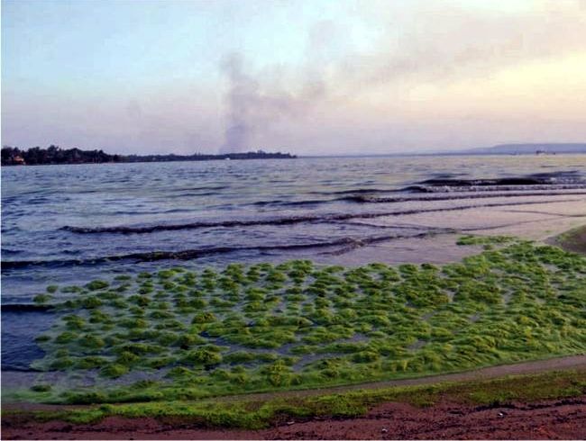
Sensors 2020, 20, 1488                                                                               3 of 28

2. Related Work
      Local planners have been studied since the birth of robotics, therefore many researchers kept
local planners evolving and also made them more efficient. Nowadays, a large amount of well-studied
methods and algorithms exist, including Dijkstra [14], Rapidly Exploring Random Trees (RRT) [15]
and Potential Fields (PF) [16].
      The goal of this work is to obtain a numerical value that represents the expected performance
of each one of the most-used path planning methods and techniques, and in that sense, several path
planners are reviewed, studied and implemented in a controlled environment for a surface vehicle.
Although there are many reviews on this topic [17,18], the focus in this work is to provide not only a
standardized path-planning testing procedure, but also results for an autonomous surface vehicle in a
low current speed environment such is the Ypacarai Lake (Paraguay). The most well-known/used
algorithms are reviewed, implemented and tested in a controlled environment.
      Dijkstra’s algorithm [14] is one of the most used path planning algorithms, it seeks a feasible path
starting from an initial position, searching in every direction for the goal position. Using a grid map,
the vehicle can implement Dijkstra to find the goal prior to any movement. Then, when the goal is
reached by the algorithm, a feasible path is returned and used by the vehicle to get to the goal position.
In recent years, practically all works use variations of the Dijkstra’s algorithm [19–21], and older ones,
like [22], use the algorithms without variations. Dijkstra’s algorithm is described in the literature as a
fast, simple path planning method.
      The RRT technique is a path planning algorithm, which is based on growing a random tree for
searching the goal position. The planner returns an obstacle-free random path. An example can be seen
in [23], which uses the RRT algorithm within an ASV to accomplish movements while adopting water
collision regulations. This technique is used in fast non-complex environments, where the vehicle
must adapt its planned movement, focusing on obtaining paths to the desired goal position and not on
the characteristics of the path (i.e., shortest, smoothest, etc.)
      PF is a path planner that creates a map that weights each point with a potential value. Generally,
it assigns lower values to the positions closer to the goal, so the vehicle should always try to move
to the minimum value, eventually reaching the goal position. To plan ahead, gradient descent is the
method used to obtain the path. Safe paths can be found as long as local minimum is not present as a
obstacle. In [24] they used PF technique to provide local paths to an underwater vehicle, also noting
that local minimum represents a problem.
      PF offers the possibility of virtual weighting. This can be considered as an advantage as it is
supposed that certain zones of the lake will not be as attractive to monitor as others because of the
presumed heterogeneous distribution of nutrients, leading to include the study of algorithms that
include weighting a map prior to calculating a path.
      Fast Marching Method (FMM) [25] is a method that considers both, the map weighting, and goal
location by solving the Eikonal Equation of wave propagation. This method extends the functionality
of both, the Dijkstra and PF techniques, but is mainly used as offline path planner because of the intense
computational power it requires. FMM is used and tested in [26], providing results that accomplish
very well the motion planning characteristics for autonomous vehicles. While the mentioned work
does not include time calculation in their performance, this information is crucial in local path planning.
In that sense, this work evaluates this method and, more importantly, proposes a modification of
the Fast Marching Square Method (FMS) to obtain faster results while maintaining other important
characteristics of the method by Updating the Fast Marching Square Method (uFMS).
      Defined in [27], path planning algorithms can be classified by the necessity of proper environment
modelling; the same survey states that, while A* does need an environment modelling, methods like
PF and RRT does not need it in order to calculate a path between two points. These methods and
their variants are defined in the same work, concluding that path planners with proper environment
modelling (i.e., regular grids) are most likely to give optimal results; while the methods without proper
modelling are more suitable for real-time requirements.
Sensors 2020, 20, 1488 4 of 28
Other works like [28] emphasize on the problem-space definition and the proven time complexity
that each algorithm has, classifying them in related groups (PF, probabilistic, cell decomposition).
In the same work, it is recommended that a solution should be chosen if it fits in the characteristics of
addressed problem.
This work surveys some of the well-known algorithms in the path-planning literature, detailing
the algorithms so they can be implemented in any programming language while also presenting their
high level characteristics like complexity and specific safety measures for autonomous surface vehicles.
Additionally, this work also takes a step further by simulating and comparing their results in a specific
scenario, facilitating the decision making for future researchers in the area.
3. Statement of the Problem
3.1. The Ypacarai Lake Contamination Problem
The objective of this paper is to perform a study of local path planning techniques and determine
the most suitable one for an ASV, particularly a catamaran, oriented for the scenario of Ypacarai lake.
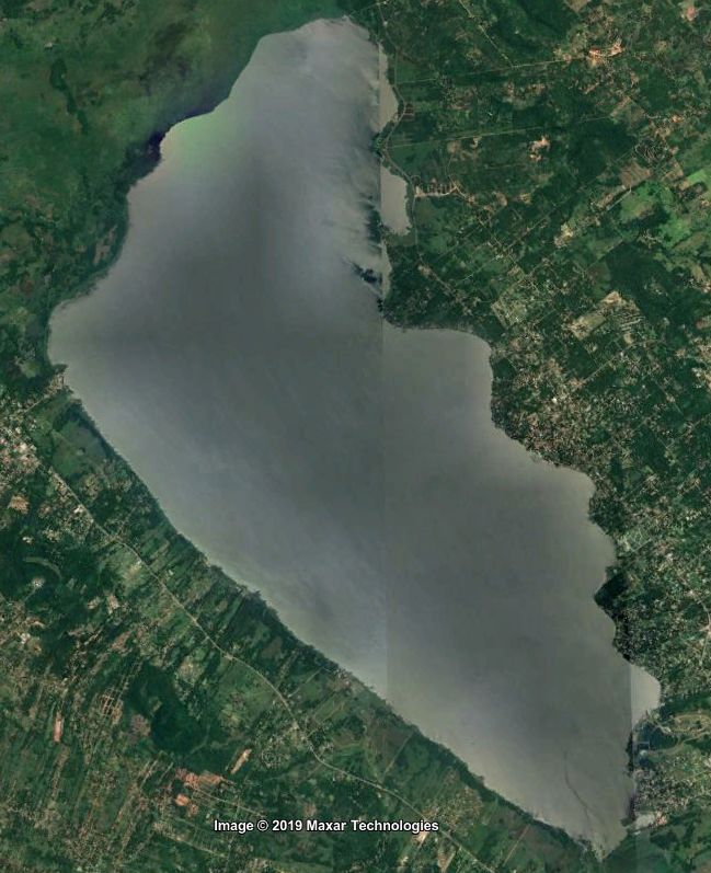
Figure 1 shows a satellite image from Ypacarai Lake taken in the end of 2018. It is a shallow lake with
an average depth of 1.72 m and a maximum depth of 2.53 m [29]. There is a large amount of population
living in the surroundings whose activities have a direct impact on the conditions of the lake. The most
notorious evidence of the degradation of the lake is the appearance of algal bloom (Figure 2), normally
in the hot season between November and December. Many monitoring campaigns were carried out
in the 1980s and more recently in this decade. Samples were taken manually at specific points in the
lake and a few fixed monitoring stations were located at the shore. However, having an autonomous
vehicle that can find its path through the lake will help in the monitoring tasks of the lake.
The problem that defines local path planning utility for monitoring applications is that, after a
global path planning is made, the vehicle should move from one target to another while avoiding any
type of obstacles, re-planning safe routes as many times as necessary. Therefore, the local path should
be as safe, direct and as fast as possible. Thus, to compare the available methods, these qualitative
characteristics should be studied with quantitative measures, whenever possible.
Figure 1. Satellite Image of Ypacarai Lake.Sensors 2020, 20, 1488 5 of 28
Figure 2. Last appearance of algal bloom at the shore of Ypacarai Lake (February 2019) [30].
3.2. Proposed Global Path Planning
An ideal global path plan for monitoring big bodies of water should contain the least amount of
information so that an Autonomous Surface Vehicle (ASV) can be tasked to cover the surface of the
body of water, or, at least, a certain amount of surface considered as sufficient. In [12], it is defined and
obtained a global path that covers the biggest area possible of the Ypacarai Lake with an ASV, using
Genetic Algorithm (GA). For this purpose, 60 waypoints or intermediate goal nodes are defined, that
the ASV should visit at least once (similar to the Travelling Salesman Problem (TSP). Then, it obtains
via a GA, a visiting order so that the ASV covers the biggest possible surface of the lake in one run.
Furthermore in [31] they proposed the use of Eulerian Circuits instead of Hamiltonian Circuits in TSP
for solving the global path planning problem. The difference of this latter approach with the TSP is
that the ASV can visit a waypoint more than once time. The resulting 60 waypoints list and the visiting
order can be fed to a local planner, the path planned, obtaining a result ready to be executed.
Though an ASV could travel directly between waypoints, some form of obstacle avoidance and/or
path modifications that considers vehicle and environment constraints should be planned ahead, to
have an estimated result prior of executing the movement. Furthermore in large maps, it is impossible
to predict dynamic obstacle presence and pinpoint the exact location of them beforehand. Therefore,
local path planning is the tool used to obtain this result.
3.3. Local Path Planning
As defined in [32], Local Path Planning is a planning method that will be responsive to obstacles
and changes of the environment, whether it is dynamic or unknown. In addition, local path planners
are known to calculate short paths, usually in the vehicle line of sight and in real time, updating the
direction of the vehicle heading if necessary. The essence of the local path can be applied to a more
broad group of path planners that track the changes of the scenario, and ask for an updated planned
path whenever the current one is no longer feasible. Additionally, this method helps to obtain more
information about the environment by storing the changes that the vehicle senses. This work studies
some of the standard local path planning algorithms and compare them in order to confidently select
a proper path planning technique to be used as local path planner in an ASV that studies the water
quality of the Ypacarai Lake.
4. Local Path Planning Algorithms
This section presents a summary of the main local path planning techniques found in the literature.
This summary includes an overview of each method together with a pseudo-code and a block diagram
describing its operation.Sensors 2020, 20, 1488 6 of 28
4.1. Pure Pursuit
Although basic Pure Pursuit (PP) is not a local path planning algorithm per se because it only tries
to reach a certain point without having a reactive behavior, it is used as starting baseline model for
comparison purposes. In fact PP is a tracking algorithm that calculates the curvature of the movement
of the vehicle from its current position to some goal point [33]. The algorithm finds some ahead point
that it is located along the path. However, in our case, no obstacle avoidance is made. Therefore,
the ASV moves directly towards each beacon or waypoint. Equation (1) shows how the velocity v is
calculated having a k gain, a target or goal, and a current position pose of the ASV. Using this equation,
Algorithm 1 is implemented to have the ASV driving from each beacon (waypoint) to another.
target − pose
v=k (1)
norm(target − pose)
Algorithm 1: Pure Pursuit
1 Require: waypoints: wp, vehicle: ASV
2 while goal ≤ t_goals do
3 pose = ASV.get_pose();
4 if pose - wp(goal) < error_allowed then
5 goal++;
6 end
7 dx = calculate_velocity(wp(goal), pose , k);
8 ASV.set_velocities(dx);
9 end
4.2. A* Planning Algorithm
A* is a local path planning algorithm that adds a heuristic function to the well known Dijkstra’s
algorithm. In the classical Dijkstra’s algorithm, it searches a route between two positions by examining
in each iteration the neighbors of a parent node, i.e., all nodes connected to the parent node or position,
and considering each neighbor as a future parent node. This process is repeated until the goal node is
found; then, a sub-function is called to find a road map with the information of the neighborhoods
found. In contrast, A* algorithm adds a priority queue, the Frontier List, which prioritizes the
examination of new nodes closer to the goal and/or with a lower cost. In this algorithm, the cost is
defined by the vehicle and/or environment restrictions and the desirable movement. Therefore, higher
costs can be assigned to nodes next to obstacles or some types of movements can be forbidden (i.e.,
crossing diagonally if there are obstacles in between). These costs are summed up and then assigned
as the priority of each new node. Thus, lower costs nodes have higher priority in the queue and have
higher chance to be the next studied or observed node. As a result, the computational total time is
reduced drastically, while maintaining the convergence and security level that the Dijkstra algorithm
offers. The complexity is known to be O( N ) with an optimal heuristic approach.
As observed in Figure 3 the algorithm follows a three-decision block sequence. The first two
are used during the creation of the map, or node graph. During these steps, the Frontier List acts
as a queue, where a node is popped and examined, and added to the Examined Node List. All of
the non-examined neighbors of this node are added to the Frontier List, for future examinations.
Then, the last decision block is found during the creation of the path, using the Examined Node List.
A pseudo-code is presented (Algorithm 2), where a priority queue of the next possible nodes to be
examined is added to finally arrive and examine the goal node. A path is then generated by calculating
the lower cost nodes that connect the goal and start nodes.Sensors 2020, 20, 1488 7 of 28
Create Frontier
Start and Examined
Node lists1
Error. No
Frontier
path between
List is
yes start and
empty?
goal position
Add neighbors no
to frontier with
node = pop
heuristic, and
from frontier
to Examined
Nodes.
Node
Get neighbors no position
of node is goal node = parent
position? of node
no
yes
Node’s
Create add node’s position
new path. position is
Origin: last to path vehicle’s
examined node. position?
yes
Return
flipped
path2
Figure 3. A* sequence diagram. 1: Both lists include the vehicle’s initial position as node. 2: The path
should go from end to start.
By modifying the Pure Pursuit runtime algorithm (Algorithm 3), the A* is implemented by adding
this planning every time the ASV reaches a goal. As observed in Algorithm 3, no major changes were
made, but A* is used for path planning. The algorithm is executed as follows. First, the goals are the
waypoints obtained from the global path planning. Between these waypoints, the p_planner (line 4 in
Algorithm 3) is executed (line 12 in Algorithm 3), which in this case is the A* algorithm. The output
of this algorithm are intermediate points that are called sub_goals. The Pure Pursuit now tracks the
direction according to these sub_goals (line 16 in Algorithm 3) instead of the goals. This procedure is
repeated until visiting all the waypoints.Sensors 2020, 20, 1488 8 of 28
Algorithm 2: A* planning algorithm
1 Require: vehicle: ASV, goal_pose: goal, map_data: map
2 vehicle_node = Node(ASV.get_pose(), parent_node=None);
3 frontier = PriorityQueue(vehicle_node);
4 examinedNodes = List(vehicle_node);
5 while frontier.not_empty() do
6 currentNode = frontier.pop();
7 if currentNode.position == goal.position then
8 examinedNodes.add(currentNode);
9 break;
10 end
11 foreach aNeighborNode in neighborNodesOf(currentNode, map) do
12 priority = get_cost_of(aNeighborNode);
13 frontier.add_with_priority(aNeighborNode, priority);
14 examinedNodes.add(aNeighborNode);
15 end
16 end
17 path_to_follow = calc_path_to_follow(examinedNodes);
18 return path_to_follow
Algorithm 3: Runtime Algorithm, including path planning
1 Require: waypoints: wp, vehicle: ASV, map_data: map
2 pose = ASV.get_pose();
3 goal = 1;
4 path = p_planner(map, pose, wp(goal));
5 sub_goal = 1;
6 while goal ≤ t_goals do
7 pose = ASV.get_pose();
8 if pose - path(sub_goal) < error_allowed then
9 sub_goal++;
10 if pose - wp(goal) < error_allowed then
11 goal++;
12 path = p_planner(map, pose, wp(goal));
13 sub_goal = 1;
14 end
15 end
16 dx = calculate_velocity(path(sub_goal), pose , k);
17 ASV.set_velocities(dx);
18 end
Algorithm 3 will be used as the base structure to build the following local path planning
techniques, only modifying the part corresponding to the p_planner.
4.3. Potential Fields Algorithm
Potential Fields (PF) path planners are widely used in robotics. The basic idea of PF consists of
defining a potential value to every point on the region by generating two types of fields, a repulsive
field and an attractive field. PF path planning is inspired by nature, more specifically, the attractive
and repulsive fields generated by electromagnetic fields. In [16] two main functions are defined,Sensors 2020, 20, 1488 9 of 28
Equations (2) and (3). Then both Uatr and Urep should be added to find a potential value for each point
x, y within the region.
1
Uatr = × k a × pdist( pose, goal ) (2)
2
kr
Urep = (3)
pdist( pose, obsti )
In these equations, k a and kr are attractive and repulsive constants, and pdist measures the
Euclidean distance between the position being examined (pose) with the goal and the obstacle i (obsti )
respectively. A procedural way for obtaining a path, can be via calculating the gradient descent of the
map. The general sequence diagram for PF path planning can be observed in Figure 4. A result of
calculating a potential map can be observed in Figure 5, where the goal was to assign small potential
value to the regions around the goal position (green star), and high potential values to regions where
the vehicle should not travel. The white color corresponds to prohibited zones or positions, like terrain,
or maybe even obstacles. Additionally, the yellow star corresponds to the starting point, which serves
no purpose while calculating the potential map.
Start
Generate map
assigning
attractive
potential
value to every
point on map
Error. No
Add repulsive
path between
potential value
start and
to every point
goal position
no
Perform
Result
gradient
OK?
descent
yes
Return
path
Figure 4. Potential Fields sequence diagram.Sensors 2020, 20, 1488 10 of 28
Figure 5. Generated potential map for a goal.
Once a potential map is generated, gradient descent can be performed from start to goal position
in order to generate a path and, if feasible, the path is given to the ASV. When the ASV reaches a
target, the next map is generated and used by the ASV. The complexity of this approach O( N log( N ))
According to [28], and since it involves the map generation and its calculation via gradient descent.
4.4. Rapid-Exploring Random Trees* Algorithm
One of the most popular sampling-based planners is the Rapid-Exploring Random Tree (RRT) [15].
The RRT algorithm grows a tree with nodes and branches connected to each other. These nodes are
created randomly and then added to the tree until a random node connects to the goal target. In order
to improve the results or creation of random nodes, RRT* [34] has been proposed as a modified version
that creates nodes within the neighborhood of a target pose, before adapting this node to the tree.
Because of the direct dependency of distance, the proven complexity is the same of A*, O( N ).
A sequence diagram for this method is presented in Figure 6, which is fairly more complex than
the previous path planners presented. This is because the method is broken into two differentiated
algorithms, excluding the main algorithm, each of them accessed depending of the decision made by
the main algorithm.
The main algorithm of RRT* can be found in Algorithm 4, then sub functions for steering and
choosing a parent in Algorithm 5 (line 7 in Algorithm 4) and Algorithm 6 (line 10 in Algorithm 4),
respectively. In the main algorithm, a tree τ is initialized, containing as main branch or root, the starting
point as a node. Then the procedure iterates by sampling or creating a new node within the region
Rn . After randomizing a sample node P (line 5 in Algorithm 4), the algorithm finds the nearest node
from tree τ (line 6 in Algorithm 4) and steers the sampled node to the nearest node, if needed (line 7 in
Algorithm 4). This steering is done in Algorithm 5, where the distance between prand and pnearest is
checked to be within certain maxStepDist distance (line 3 in Algorithm 5). If not, a new point psteer is
generated by defining its direction to be the same as the vector difference between pnearest and prand ,
and the magnitude equal to maxStepDist; this psteer is assigned as the new prand . Back in the main
algorithm, it is checked if there is a feasible route between pnearest and prand , after that. The function
chooseParent (line 10 in Algorithm 4) obtains the parent with the lower cost and, as [34] suggests,
the new node should be connected to the best parent using the Algorithm 6, which calculates the lower
cost of connection to a parent and returns this parent. The same work defines the cost of a new node
as the distance between the new point and a node of the tree. Finally, the new node is added to theSensors 2020, 20, 1488 11 of 28
tree and connected to its best parent together with the calculated cost. Afterwards, the procedure
repeats until a 2020,
Sensors random
xx, 5 node is located within the position of the goal or desired position. 11 of 30 Then,
the path should travel from the last created node to the starting node. In order to improve results,
the randomized newtravel
path should nodefrom
could be randomly
the last created node sampled to be
to the starting theIngoal
node. orderposition.
to improveRRT is one
results, the of many
randomized
path planners new node
that returns ancould
“anybe angle
randomly sampled
path”, to be the that
meaning goal position. RRT isisone
the vehicle of many
able and path
instructed to
planners that returns an “any angle path”, meaning that the vehicle is able and instructed to travel in
travel in any direction, unlike the previous planners that may travel only in several discrete directions.
any direction, unlike the previous planners that may travel only in several discrete directions.
Start
Create root
w/ starting
position
New Create new
Randomize no node path. Origin:
a new node is goal yes last node
node? created.
Steer new node
Is Insert new add node’s
close to nearest.
feasible node w/ position
Select best yes
path? Best Parent to path
parent node.
Node’s
Return position
flipped is
yes
path1 vehicle’s
position?
no
node = parent
of node
Figure 6. RRT* sequence diagram. 1: The path should go from end to start.
Figure 6. RRT* sequence diagram. 1: The path should go from end to start.
Algorithm 4: Main algorithm for RRT*
1 Require:vehicle: ASV, goal_position, max_iterations: m_i
2 τ = initializeTree();
3 insertNode( ASV.get_pose(), τ );
4 for i=1: iSensors 2020, 20, 1488 12 of 28
Algorithm 5: Rapidly-Exploring Random Trees (RRT) steering function.
1 Require: Tree: τ, new_point: pnew , nearest_point: pnearest
2 pos = pnew .position;
3 if dist(pnearest , pnew ) > maxStepDist then
4 θ = atan(pnew .position, pnearest .position);
5 pos = pnearest .position + sign(pnew .position-pnearest .position)*max_step*angles(θ);
6 end
7 return pos
Algorithm 6: Obtaining the best parent node for a new node
1 Require: new_point: pnew , near_nodes: pnearNodes , nearest_node: pnearest
2 best_pt = pnearest ;
3 min_cost = pnearest .cost + dist(pnearest .position - pnew .position);
4 foreach pnear in pnearNodes do
5 t_cost = pnear .cost + dist(pnear .position - pnew .position);
6 if t_cost < min_cost then
7 [min_cost, best_pt] = [t_cost, pnear ];
8 end
9 end
10 return best_pt
4.5. Fast Marching Method and Variations
4.5.1. Fast Marching Method and Fast Marching Square Method
The Fast Marching Method [25] is an offline path planning algorithm, which solves efficiently the
Eikonal Equation (Equation (4)), computing the propagating fronts of a wave.
|∇ T ( p)|V ( p) = 1 (4)
where T ( p) represents the arrival time to point p, V ( p) is the propagating velocity at point p, and ∇ the
gradient. The FMM algorithm proposes to discretize Equation (4) to calculate T ( p) ∀ p( x, y) by using
a map M, which contains all points p ∈ Rn , and defining ∆x and ∆y as minimun possible movements.
The last description can be used to define von Neumann’s neighbors of a point p as ( x + ∆x, y),
( x − ∆x, y), ( x, y + ∆y) and ( x, y − ∆y). Finally, according to [26], the value of T ( p) can be found using
the following equations:
T1 = min( T( x+∆x,y) , T( x−∆x,y) ) (5)
T2 = min( T( x,y+∆y) , T( x,y−∆y) ) (6)
T( x,y) − T1 T( x,y) − T2 1
( )2 + ( )2 = (7)
∆x ∆y (V(x,y) )2
The solution of these equations is given by:
1
T1 + V(x,y) , if T2 ≥ T ≥ T1 .
T( x,y) = T2 + V 1 , if T1 ≥ T ≥ T2 . (8)
( x,y)
Solution o f Equation (7),
if T > max ( T1 , T2 ).Sensors 2020, 20, 1488 13 of 28
This equation is known as the Cost Update function, and will be the function that calculates
the time of arrival or cost update for every point in the region. In the FMM algorithm, the velocity
matrix V( x,y) takes binary values (0 or 1), where its dimensions correspond to the map M dimensions.
The ∆ step is defined to be the same in both, x and y directions, and equal to the unitary value to
facilitate the solving of the Equations (5)–(8). In order to determine the correct values in an iterative
way, the order of obtaining these values must coincide with the propagation of this hyper surface.
Therefore, the values must be calculated from a starting point outward. Thus, it can be said that the
resolution of the FMM is similar to the resolution of the Dijkstra but in a more continuous way.
Figure 7 shows the sequence diagram to obtain the Time Of Arrival (TOA) matrix. This algorithm
requires an initial point (or points) and a velocity map, and returns the TOA matrix, which can be
considered as the final matrix to calculate the route.
Initialize
Start
TOA matrix
Select VNN1 of
initial point(s),
calculate their
TOA, add
points to trial
Trial Return
yes Time of
queue is
empty? Arrival
Matrix
no
Select VNN of Select lowest
point, calculate cost point
their TOA, add and remove
points to trial from trial
Figure 7. FMM: Procedure to find Time of Arrival (TOA) matrix. 1: Von Neumann’s Neighbors.
This approach is presented in Algorithm 7, taking into account that the time of arrival Tp0 to the
starting point is always zero (line 3 in Algorithm 7). Then between lines 5–9 a trial queue is built with
the VNN of the starting point p_start, and from there all the arrival times of the remaining points of
the map are calculated with the cost_update() from Equation (8) (line 19 of Algorithm 7. The algorithm
also checks if there are undefined points with cost → ∞ (line 13 in Algorithm 7).Sensors 2020, 20, 1488 14 of 28
Algorithm 7: Solving Fast Marching Method (FMM) Time of Arrival matrix.
1 Require: Starting Point: pstart , Velocity Map: vmap
2 toa = new_matrix(vmap .size());
3 toa(pstart ) = 0;
4 trial_queue = PriorityQueue();
5 foreach neighbor in vn_neighbors(pstart ) do
6 time_to_p = cost_update(neighbor, toa, vmap );
7 trial_queue.add_with_priority(neighbor, time_to_p);
8 toa(neighbor) = time_to_p;
9 end
10 while trial_queue.not_empty() do
11 next_point = get_lowest(trial_queue, toa);
12 trial_queue.remove(next_point);
13 if next_point.cost == inf then
14 break;
15 end
16 foreach n in vn_neighbors(next_point) do
17 if toa(n) == undefined then
18 t_to_p = cost_update(n, toa, vmap );
19 trial_queue.add_with_priority(n, time_to_p);
20 toa(n) = t_to_p;
21 end
22 end
23 end
24 return toa
Fast Marching Square Method (FMS) is a variation of the same method that performs the FMM
twice. The procedure can be observed in Figure 8. The Algorithm 8, extracted from [26], shows that
the same method is used twice, the first time it uses the Cost Function to calculate the velocity map
(using Equation (8) with the TOA matrix as result, line 2 in Algorithm 8); setting any present obstacle
as generators or initial points. So Algorithm 7 must be prepared to receive as initial state more than
one point. Then, from those points the velocity map is generated (line 3 in Algorithm 8). With the
calculated velocity map, the algorithm proceeds the same as the usual FMM, assuring a modified
velocity at all positions that are in the presence of obstacles (line 4 in Algorithm 8). Most likely the
map will be different from the binary map used in the previous method.
There is a different time complexity for these methods because of map calculations; while
FMM requires a single map calculation, FMS requires two, so the complexity of these methods
are O( N log( N )) and O( N 2 log( N )) respectively.Sensors 2020, 20, 1488 15 of 28
Start
Calculate
speed matrix
w/ obstacles
as generators.
Calculate
TOA matrix
Perform
gradient
descent
Return
Path
Figure 8. FMS sequence diagram.
Algorithm 8: Fast Marching Square Method.
1 Require: Initial Map: M, Starting Point: pstart , Goal Point: p goal
2 V = calculate_speed_matrix(M);
3 OB = perform_fmm(pobstaclei , V);
4 TOA = perform_fmm(pstart , OB);
5 path = gradientDescent (TOA, pstart , p goal );
6 Return: path;
4.5.2. Proposed uFMS
Updated Fast Marching Square Method (uFMS) is proposed in this work to improve the efficiency
and effectiveness of the FMS by using local methods of updating the generated maps. As the original
method, it is divided into two fundamental parts but it is focused on drastically decreasing the total
time to generate a route by updating only zones or regions that present new information.
The main problem to mitigate in FMM or FMS is that the entire TOA matrix should be calculated
even if the difference between some previous map and a new one is small (new obstacles, new free or
occupied zones). To solve this problem, the uFMS algorithm saves the map previously generated by
the FMS method, and updates both matrices (velocity and TOA), exclusively in a defined region that
contains the modification of the map.
As a first instance, the region to be modified is defined by a position to update pnew and an update
radius ρ. For this, two vectors containing the horizontal and vertical distances d x and dy from pnew to
all points p of m are generated. Then, a radial mask is generated with Equation (9).
∀ d2x + d2y ≤ ρ2 .
(
1,
mask = (9)
0, else.
which provides the values that are at a distance less than or equal to a defined radius, forming a
radial mask. This mask is used as base to determine which values should be recalculated in the TOA
and velocity matrices, redefining these values as undefined. The sequence diagram can be observed
in Figure 9. The Algorithm 9 also shows the procedure. It is worth noting the similarity with the
FMS (Algorithm 8), but the requirements change as the information of a previous map is necessary.
The alteration point and a radius are also added and considered for solving the algorithm. Moreover,Sensors 2020, 20, 1488 16 of 28
instead of the usual calling of update_ f mm() function, an update_ f mm() function (found at lines 3
and 5) is used, which adds the functionality of modifying strictly the previous map through the use of
the Equation (9). It is also important to note that a function is added to apply a Gaussian filter (lines
4 and 6 of Algorithm 9), to smooth the result, which is necessary to improve the costs calculated for
arrival times and the response of the descending gradient. The update_ f mm() function is presented in
Algorithm 10, which presents some slight crucial modifications.
Start
Update initial
velocity map
Update speed
matrix w/
obstacles
Apply
Gaussian
filter to
speed matrix
Update FMM
Apply
Gaussian
filter to TOA
Perform
gradient
descent
Return
Path
Figure 9. uFMS sequence diagram.
Algorithm 9: Updating Fast Marching Square Method.
1 Require: Starting Point: pstart , Goal Point: p goal , Information from last map: (TOA, OB, V),
Modification Point: pnew , Modification Radius: ρ
2 update_velocity_map(V, pnew );
3 OB = update_fmm(OB, V, pnew , ρ);
4 OB = apply_gaussian_filter(OB);
5 TOA = update_fmm(TOA, OB, pnew , ρ, pstart );
6 TOA = apply_gaussian_filter(TOA);
7 return path, TOA, OB, VSensors 2020, 20, 1488 17 of 28
In this algorithm, lines 3–9 impose the restriction that the map must obtain the new values only
within the desired zone. The rest of the algorithm is equal to Algorithm 7. All these changes can be
observed in the sequence diagram in Figure 10. Since FMS and uFMS in static conditions will provide
the same results, the result of running this algorithm will produce the same output.
Algorithm 10: Updating procedure in Updating Fast Marching Square Method (uFMS).
1 Require: Current TOA: toa, Velocity map: v, Modification Point: pnew , Modification Radius: ρ,
Starting Point: pstart
2 trial_queue = PriorityQueue();
3 d x , dy = distance_from_point(v, pnew );
4 mask = d2x + d2y ≤ ρ2 ;
5 toa(mask) = undefined;
6 if pstart is null then
7 toa(pnew ) = 0;
8 pstart = pnew ;
9 end
10 foreach neighbor in vn_neighbors(pstart ) do
11 time_to_p = cost_update(neighbor, toa, v);
12 trial_queue.add_with_priority(neighbor, time_to_p);
13 toa(neighbor) = time_to_p;
14 end
15 while length_of(trial_queue) > 0 do
16 next_point = get_lowest(trial_queue, toa);
17 trial_queue.remove(next_point);
18 if next_point.cost == inf then
19 break;
20 end
21 foreach n in vn_neighbors(next_point) do
22 if toa(n) == undefined then
23 t_to_p = cost_update(n, toa, v);
24 trial_queue.add_with_priority(neighbor, t_to_p);
25 toa(n) = t_to_p;
26 end
27 end
28 end
29 return toaSensors 2020, 20, 1488 18 of 28
Create and
apply update
Start
region mask
to TOA matrix
Select VNN1 of
initial point(s),
calculate TOA,
add to trial
Trial yes Return
queue is TOA
empty? Matrix
no
Select VNN
Select lowest
of point,
and remove
calculate TOA,
from trial
add to trial
Figure 10. uFMS: Procedure to update TOA matrix.
5. Evaluation of Local Path Planning Algorithms
Validation of motion planning techniques are a main concern nowadays, because of the existence
of a considerable amount of path planning algorithms in the state-of-the-art. In that sense, this works
presents a formal generalized way to obtain the performance value of some path planning techniques.
This is achieved by defining the vehicle, the environment in which the vehicle will move and a
measuring system.
The first approach on evaluating robotics procedures is through simulation. Although it does
not represent the real world, it provides a safer, cheaper and controllable way of testing data.
For this reason, in this work, the algorithms are tested and measured using a simulation environment,
based on the Robotarium Framework [35]. The Robotarium Framework provides a 2-D environment
and simulated 2WD-vehicles; both of these characteristics were ported to the developed simulator in
our research laboratory. In addition to the characteristics previously mentioned, control systems and
measuring systems were added to obtain a proper testing environment. The simulation environment
is defined in Section 5.1, while the simulation procedures and the simulation results are defined in
Sections 5.2 and 5.3, respectively.
5.1. Simulation Environment
All path planning algorithms require data of the world space in which the vehicle moves. In this
work, this data is comprised in a m by n matrix, simulating a 2-D environment (Euclidean plane),
where the vehicle is always located within a point p ∈ R2 . Furthermore, the most common method of
Cell Decomposition is used as all pi,j elements of the world space representation matrix are regular in
size, shape and arrange. This decision facilitates the use of any image since a y, x pixel of the image
will correspond directly to a pi,j element of the matrix.
Particularly, an image of the Ypacarai Lake in black and white was obtained using an online
tool [36], resulting in a reliable representation, where a black pixel corresponds to land and a white
pixel to water. This is generalized where white pixels represents free from collision or reachable
positions and black represents obstacles, unreachable zones, prohibited areas, etc. This image has aSensors 2020, 20, 1488 19 of 28
dimension of 1000 by 1500 pixels, where the distance between the center of adjacent pixels measures
roughly 10.33 m. This distance is a very important value because it defines the resolution of the
framework, which inherently affects the level of adaptability of the studied methods. This statement
will be discussed in the following paragraphs, as it also depends on the kinematics of the vehicle.
It is worth noticing that the vehicle could be located anywhere in the map within a pixel p. This is
because the vehicle is represented as a point in this context, and due to the fact that the real ASVs to
be tested have small dimensions (2–4 m) compared to the pixel size. In the simulation environment,
this vehicle is capable of moving according to a set of constraints and configurations that properly
models a real ASV. After a path is planned, the ASV obtains the direction to travel to a specific goal
position. This direction consists on a 2-dimensional vector that contains the information of the desired
velocity V.
~
As all real systems cannot accomplish to reach desired values perfectly, the simulated vehicle
takes this into account by assigning a function that maps desired velocities to modelled “real” values.
The simulated vehicle corresponds to a catamaran, a double-hull boat with separated propulsion
systems, one on each hull. This configuration allows the vehicle to rotate on its center, which
corresponds to unicycle dynamics. A proper model definition is available in [37]. The unicycle
model uses the information of the vehicle desired velocity as well as its orientation (rotation angle
with respect to a horizontal line, θ), obtaining a linear velocity v and an angular velocity ω calculated
with the set of equations Equations (10)–(12) where k v and k ω correspond to velocity limits.
A = (cos θ, sin θ ) (10)
v = k v ( A1 V
~ x + A2 V
~y) (11)
arctan(− A2 V ~ y , v)
~ x + A1 V
ω = kω π (12)
2
This v, ω velocity pair is suitable to approximate the movement of an ASV, and it should be
fed to a movement simulator environment, that updates the position of the vehicle after a certain ∆t
time-step. In this particular setup the time-step is 1/12,551 s, and the linear velocity equals to 0.033
pixels/time-step. These are the default values found in the Robotarium framework.
A fully-functional simulator has been developed in Python which also provides visualization
and some defined measuring performance parameters [38]. The simulator also updates the state or
position of the simulated ASV according to the angular and linear velocities updated in each step, and
to kinematics of the vehicle. Furthermore, the simulator comprises a kinematics system to update
the position of the vehicle, a localization system, including a map and a simulated LIDAR system, a
visualization system, to produce visual output, and an auxiliary evaluation system, for evaluation
purposes. The kinematics system includes simple functions to calculate the position of the simulated
vehicle, taking into account a model of surface vehicles with their respective maximum velocities,
turns and constrains. On every step, this system calculates and updates the position of the vehicle
accordingly. The simulator map requires an image file, preferably monochromatic, in which the free
zones and obstacles zones are clearly differentiated, (i.e., black and white tiles) and information about
which tiles are obstacles. The simulator stops if the vehicle is not located in a free zone.
5.2. Simulation Procedures
As this work pursues the selection of an appropriate Local Path Planning technique for monitoring
application of the Ypacarai Lake, a simple model of the lake was obtained and fed as an image into the
simulator, with shores as obstacle zones, and water as free zones. The mission of the simulated ASV
was to travel from one waypoint to another using the 60 waypoint system as in [12], rearranged to
fit the model of the lake. These beacons were placed near the shore, inside the lake, considering the
transmission range of wireless RF technology modules (e.g., Xbee [39]), using the procedure shown
in [38], so that distances between adjacent beacons were equal or lesser than the maximum rangeSensors 2020, 20, 1488 20 of 28
(1000 m). The purpose was that, in a real application, these waypoints formed a multi-hop network
so the ASV could transmit the sensed data to a base station. These waypoints were used as goal
positions and the mission was considered as complete whenever the vehicle visited all 60 waypoints
at least once.
After this initialization, the main Algorithm 3 ran and the position of the ASV was updated right
after the ASV.set_velocities(dx ) function (line 17), so the simulator continuously checked whether the
ASV reached the current goal, and responded accordingly.
In order to compare methods, each of the path planners (A*, PF, RRT*, FMS and uFMS) were
called in lines 4 and 12 of Algorithm 3 for 10 different possible global path solutions. For the sake
of comparison, several performance parameters were measured, such as the time of path planning,
the total simulation time, the difference in the distance with the ideal path, and the security levels.
Then, each of these values were normalized and equally weighted in order to provide a grade in a
scale from 0 to 100, being the best technique the one with the greatest number.
The measured parameters by the evaluation system included the following:
1. Time of Path Planning: measured whenever the vehicle started to plan a new path until the
calculation was done and a valid path was obtained. This measure shows the path planner time
complexity. Ideally, path planners used a little amount of time to calculate a path, and as Pure
Pursuit algorithm did not compute any path planning, it can be used as standard or ideal time
(0 s). As the distance varied between waypoints, the average values were calculated.
Equation (13) was used to obtain a normalized and weighted value. In this equation, t pp refers
to the mean time of path planning, w to a weighting constant and t ppmax the maximum allowed
value of mean time of path planning. It is important to emphasize that the weighting constant
was equal to 25 as there were four evaluation parameters, giving a maximum total of 100 when
added. Additionally, the maximum allowed time was defined to keep the values in the same
order of magnitude.
w
twpp = × (t ppmax − t pp ) (13)
t ppmax
2. Total Simulation Time: As every path planner generally generated a different path, the total
simulation time tst , including the first criterion and also the time it took to travel through the
planned path, should also be considered, since the planner could return an obstacle-free path
that took longer time which is not optimal. The function for obtaining this value (Equation (14))
slightly varies from the previous one because there is a minimum total simulation time given by
the solution of the Pure Pursuit algorithm, which is different from zero. The maximum value is
also different as it represents a random maximum simulation time to accomplish the objective.
w
twst = (tstmax − tst ) (14)
tstmax − tstmin
3. Difference in Distance Driven: Because of specifics of the work in [12], the real traveled path
should be as equal as possible as the path calculated by the GA global path planner, in which
direct routes from waypoint to waypoint were assigned. Environment modeling does contribute
on generating different routes than those of a straight line, but path planners generally do not
provide this straight, direct routes between two points because of procedures. Measuring the
difference of the distance between two points disti , and the real distance traveled between the
same points disttravel i is important because it provides a way to measure the change of global
path planning versus the executed path.
A way to obtain a weighted value of this measure is calculating first the average value between the
n extra traveled distance (difference between traveled distance and calculated distance for everySensors 2020, 20, 1488 21 of 28
route i in n) and calculated distance between points for every path, Equation (15). Afterwards,
the weighted can be calculated with Equation (16), with a maximum ddi f wmax allowed.
disttravel −disti
∑in=1 i
disti
m_di f = (15)
n
w
ddi f w = × (ddi f wmax − m_di f ) (16)
ddi f wmax
4. Security Level: As the path planning algorithms generally do not take into account the dynamics
of the vehicle, this criterion rated the level of security, or how secure it is to execute the planned
path. The generated paths were rated observing generated path and assessing its quality through
a weighted value according to the items below:
• Level 5: The path contains no drastic turns or maneuvers that an ASV cannot handle,
the path avoids obstacles easily and prevents the ASV from collision.
• Level 4: The path generally contains maneuvers that an ASV can handle and execute, all
obstacles are avoided but the ASV can travel very close to them.
• Level 3: The path contains drastic turns and maneuvers that an ASV cannot handle easily,
obstacles are avoided but the ASV can travel very close to them.
• Level 2: The path contains turns and maneuvers that are very hard to be executed on an
ASV, obstacles whatsoever are avoided.
• Level 1: The path contains maneuvers that are not possible on an ASV, crosses an obstacle or
does not take into account any obstacle present.
The security level is the only criteria adopted that is not generalized to any kind of vehicle,
because it heavily depends on the vehicle dynamics. The security level should be previously defined
for every type of vehicle, taking into account the safeness need and the vehicle dynamics.
With the procedures and criteria properly defined, the simulations were executed. The simulator
was written and run in Python 3.6.5, in a Windows 10 x64 OS, and in a machine with the following
specifications: CPU Intel Core i7-7700HQ @ 2.8 GHz and 8 Gb RAM memory. The simulator as well as
the path planners and examples codes can be found in [40].
All path planners used the same set of waypoints in each simulation, and visited each of them
in the same order. The goal of the ASV was to visit each waypoint once, and when one was visited,
a path to the next waypoint was calculated and the calculation time measured. In every iteration,
the distance traveled in a delta time step was stored and added to the total. Tables 1 and 2 show the
parameters used in the simulation environment and the configurations parameters used to calculate
the performance of the path planners according to the aforementioned performance metrics.
Table 1. Simulation Parameters.
Number of simulations 10
Number of waypoints 60
Map size (pixels) 1000 × 1500
Pixel Size (meters) 10.33
ASV linear velocity (pix/time-step) 0.033
Time-step (µseconds) 79.68Sensors 2020, 20, 1488 22 of 28
Table 2. Weight normalization parameters.
Weight factor - w 25
Path planning maximum time (s) - t ppmax [s] 100
Simulation maximum time (s) - tstmax [s] 10,000
Maximum difference distance (pixel) - ddi f wmax [%] 50
5.3. Simulation Results
Before any specific discussion on the proposed methods, the discussion focuses on the parameters
for both Tables 1 and 2. A total of 60 simulations were run and all of them achieved the goal of
visiting the waypoints in the established order. As the error allowed (recall Algorithm 3) was the
same for all methods (error_allowed = 0.01pix), and the same kinematics model and parameters
were used, the comparison between algorithms is impartially devoted to the qualitative-quantitative
characteristics of each method.
First, in order to illustrate the obtained results with the different local path planning techniques
are presented, the Figure 11 is presented. Figure 11a was generated example by running the PP
algorithm, which are basically the routes generated by connecting two consecutive waypoints with
a straight line. Second, Figure 11b was generated by running the A* algorithm, with the planned
path as the red lines and the waypoints as red circles. It is important to notice that new intermediate
waypoints were created with this kind of procedure, because of the nature of grid based searching
algorithms, the movements of the vehicle were constrained to eight possible movements, one on each
direction of the direct neighbors of the node. In this case, there was a neighbor every 45◦ , starting
from zero, since the map was divided into regular square shapes. Figure 11c shows the resulting path
using PF. As there were no obstacles in this preliminary maps, the path also had straight lines between
waypoints. Then, Figure 11d shows the generated path by RRT*. It is very clear that this algorithm
added many unnecessary nodes, but provided a more direct route than A* for every target. Finally,
Figure 11e, shows a curved path generated by the FMS and uFMS algorithm. This curve was generated
due to the smoothing effect of the Cost Function.
Second, the numerical results of the performance evaluation for each path planning algorithm are
shown in Table 3. Although the Pure Pursuit algorithm was not a local path planner, it is included in
the Table 3 as a baseline for the sake of comparison. Among the local path planning methods, RRT*,
and A* took the lower average time of path planning necessary to produce outputs whenever a new
obstacle was detected. The total simulation time of these path planning methods were also fairly
similar. PF calculated the most direct route (lowest difference in distance), however its computation
time was much higher than A* and RRT*. FMS and uFMS produced routes within the same levels of
difference in distance of RRT*, both higher than A*. This statement seems to contradict the qualitative
analysis that can be made by observing Figure 11b,e, but generally the uFMS planned paths were
longer than the paths generated by A* method. Figure 12 shows another example of routes generated
with A* and FMS/uFMS, where it is clearly seen that the planned path with A* was shorter in length
but FMS/uFMS produced a safer one. The extremely high computation time for FMS makes it
unsuitable to act as path planner in our scenario. However, the proposed uFMS reduced dramatically
the computation time of the original FMS (see Table 3).
In terms of security level FMS and uFMS were the only methods that accomplish Level 5 of
security, A* and PF methods heavily depended on the environment, they generally avoided obstacles
but the ASV traveled very close to them (see Figure 12). The paths that RRT* generated contained
many intermediate waypoints that were not in the same line, that caused the vehicle to take many
turns and maneuvers to reach the waypoint.
For a further performance analysis of these methods, all the results were weighed and added on
a scale of 100, with a maximum of 25 for each criterion. A summary of the statistics of the multiple
simulations are shown in Table 4 and the generated stacked bar graph can be observed in Figure 13. It
is seen that the highest grades were achieved by the A* and the proposed uFMS. The A* had a slightlyYou can also read