Earth's Time-Variable Gravity from GRACE Follow-On K-Band Range-Rates and Pseudo-Observed Orbits - MDPI
←
→
Page content transcription
If your browser does not render page correctly, please read the page content below
remote sensing
Article
Earth’s Time-Variable Gravity from GRACE Follow-On K-Band
Range-Rates and Pseudo-Observed Orbits
Igor Koch * , Mathias Duwe                   , Jakob Flury        and Akbar Shabanloui

                                          Institut für Erdmessung, Leibniz Universität Hannover, 30167 Hannover, Germany;
                                          duwe@ife.uni-hannover.de (M.D.); flury@ife.uni-hannover.de (J.F.); shabanloui@ife.uni-hannover.de (A.S.)
                                          * Correspondence: koch@ife.uni-hannover.de

                                          Abstract: During its science phase from 2002–2017, the low-low satellite-to-satellite tracking mission
                                          Gravity Field Recovery And Climate Experiment (GRACE) provided an insight into Earth’s time-
                                          variable gravity (TVG). The unprecedented quality of gravity field solutions from GRACE sensor
                                          data improved the understanding of mass changes in Earth’s system considerably. Monthly gravity
                                          field solutions as the main products of the GRACE mission, published by several analysis centers
                                          (ACs) from Europe, USA and China, became indispensable products for quantifying terrestrial water
                                          storage, ice sheet mass balance and sea level change. The successor mission GRACE Follow-On
                                          (GRACE-FO) was launched in May 2018 and proceeds observing Earth’s TVG. The Institute of
                                          Geodesy (IfE) at Leibniz University Hannover (LUH) is one of the most recent ACs. The purpose of
                                          this article is to give a detailed insight into the gravity field recovery processing strategy applied at
                                          LUH; to compare the obtained gravity field results to the gravity field solutions of other established
                                ACs; and to compare the GRACE-FO performance to that of the preceding GRACE mission in terms

                                          of post-fit residuals. We use the in-house-developed MATLAB-based GRACE-SIGMA software to
Citation: Koch, I.; Duwe, M.; Flury,      compute unconstrained solutions based on the generalized orbit determination of 3 h arcs. K-band
J.; Shabanloui, A. Earth’s
                                          range-rates (KBRR) and kinematic orbits are used as (pseudo)-observations. A comparison of the
Time-Variable Gravity from GRACE
                                          obtained solutions to the results of the GRACE-FO Science Data System (SDS) and Combination
Follow-On K-Band Range-Rates and
                                          Service for Time-variable Gravity Fields (COST-G) ACs, reveals a competitive quality of our solutions.
Pseudo-Observed Orbits. Remote Sens.
                                          While the spectral and spatial noise levels slightly differ, the signal content of the solutions is
2021, 13, 1766. https://doi.org/
10.3390/rs13091766
                                          similar among all ACs. The carried out comparison of GRACE and GRACE-FO KBRR post-fit
                                          residuals highlights an improvement of the GRACE-FO K-band ranging system performance. The
Academic Editors: Lucia Seoane and        overall amplitude of GRACE-FO post-fit residuals is about three times smaller, compared to GRACE.
Guillaume Ramillien                       GRACE-FO post-fit residuals show less systematics, compared to GRACE. Nevertheless, the power
                                          spectral density of GRACE-FO and GRACE post-fit residuals is dominated by similar spikes located
Received: 26 March 2021                   at multiples of the orbital and daily frequencies. To our knowledge, the detailed origin of these
Accepted: 27 April 2021                   spikes and their influence on the gravity field recovery quality were not addressed in any study so
Published: 1 May 2021                     far and therefore deserve further attention in the future. Presented results are based on 29 monthly
                                          gravity field solutions from June 2018 until December 2020. The regularly updated LUH-GRACE-FO-
Publisher’s Note: MDPI stays neutral
                                          2020 time series of monthly gravity field solutions can be found on the website of the International
with regard to jurisdictional claims in
                                          Centre for Global Earth Models (ICGEM) and in LUH’s research data repository. These operationally
published maps and institutional affil-
                                          published products complement the time series of the already established ACs and allow for a
iations.
                                          continuous and independent assessment of mass changes in Earth’s system.

                                          Keywords: GRACE follow-on; gravity field recovery; time-variable gravity; satellite gravimetry;
                                          dynamic orbit determination; satellite-to-satellite tracking; KBRR post-fit residuals
Copyright: © 2021 by the authors.
Licensee MDPI, Basel, Switzerland.
This article is an open access article
distributed under the terms and
                                          1. Introduction
conditions of the Creative Commons
Attribution (CC BY) license (https://         The two identical satellites of the twin satellite mission Gravity Recovery and Cli-
creativecommons.org/licenses/by/          mate Experiment (GRACE) [1] were orbiting the Earth from March 2002 until December
4.0/).                                    2017/March 2018 (GRACE-B/GRACE-A) in a near-circular and near-polar low Earth orbit

Remote Sens. 2021, 13, 1766. https://doi.org/10.3390/rs13091766                                       https://www.mdpi.com/journal/remotesensing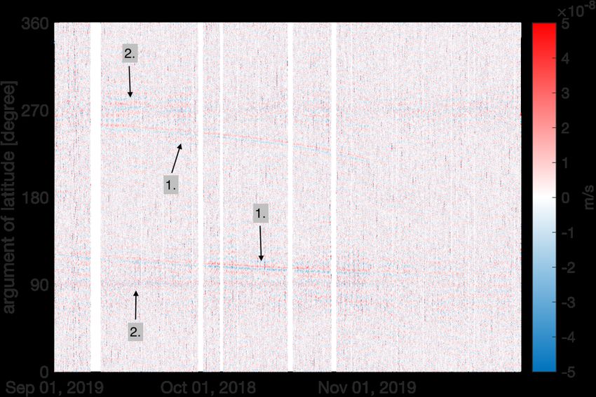
Remote Sens. 2021, 13, 1766                                                                                           2 of 23

                              (LEO), most of the time separated by a distance of approximately 220 km. The relative
                              position change of the two satellites in terms of the inter-satellite range was measured by a
                              microwave K/Ka-band ranging (KBR) system with a micron level precision. This principal
                              measuring technique—the low-low satellite-to-satellite tracking—was established for the
                              first time on a geodetic satellite mission, and in combination with additional scientific pay-
                              load [2,3], revolutionized the monitoring of Earth’s gravity variations from space. Based on
                              the processing of inter-satellite ranging measurements and data of additional sensors such
                              as Global Navigation Satellite Systems (GNSS) receivers (absolute position), accelerometers
                              (non-gravitational accelerations) and star cameras (satellite’s orientation in space), several
                              analysis centers (ACs) published time series of gravity field solutions, typically with a
                              temporal resolution of one month, e.g., [4–14], as well as (combined) long-term mean
                              models, e.g., [15–17]. Improvements in background force models such as the ocean tide
                              models, e.g., [18,19], and models of short term non-tidal variations of the oceans and the
                              atmosphere, e.g., [20,21], and advances in sensor data processing and parameter estimation,
                              e.g., [22–24], led to the publication of several generations of solutions with increasing
                              quality and resolution. Since gravity field variations are caused by mass changes in Earth’s
                              system, the monthly solutions obtained from GRACE measurements are essential and
                              valuable products for a wide range of research fields related to the hydrosphere, cryosphere
                              and lithosphere [25]. The gravity field solutions help to quantify terrestrial water storage
                              changes, e.g., [26–31], monitor ice sheet and glacier mass balance, e.g., [32–36], and the
                              mass contribution to sea level change, e.g., [36–39].
                                    The successor GRACE Follow-On (GRACE-FO) mission was launched in May 2018
                              and proceeds observing Earth’s changing gravity. Apart from minor modifications, the
                              proven orbit design, spacecraft design and scientific payload of the GRACE mission,
                              with the microwave sensor as the primary ranging instrument, were retained, e.g., [40].
                              For the purpose of technology demonstration for future satellite gravimetry missions and
                              space-based gravitational wave detection missions, a laser ranging interferometer (LRI)
                              with improved ranging precision was placed onboard [41,42]. The performance of almost
                              all instruments meets expectations and is consistent or slightly better compared to the
                              preceding GRACE mission [40,42]. However, since the end of June 2018, a severe degra-
                              dation of accelerometer measurements on one of the twin satellites is observed, which
                              manifests in higher noise and bias jumps, usually occurring during thruster firings [40].
                              GRACE-D accelerometer measurements currently do not contribute to accelerometer prod-
                              ucts standardly used for gravity field parameter estimation (Level-1B products). Instead,
                              accelerometer products (ACT1B) based on a transplantation of GRACE-C measurements
                              are published [24,43,44]. Despite these new challenges, the monthly gravity field solutions
                              published up to date, show a high level of consistency with previous GRACE results,
                              e.g., [40].
                                    The Institute of Geodesy (IfE) at Leibniz University Hannover (LUH) is one of the most
                              recent GRACE and GRACE-FO ACs. An initial time series of GRACE monthly gravity field
                              solutions was released in 2018 [13,14]. The solutions were computed with the in-house-
                              developed GRACE-SIGMA (GRACE-Satellite Orbit Integration and Gravity Field Analysis
                              in Matlab) software package, which utilizes the generalized dynamic orbit determination
                              with variational equations for gravity field recovery (GFR). Many aspects of LUH’s GFR
                              processing strategy applied for GRACE were revised. The main improvements concern
                              the background force modeling, parametrization of satellites’ accelerometer calibration
                              parameters, data screening and outlier detection. This revised processing strategy is
                              currently applied for LUH’s first release of GRACE-FO monthly gravity field solutions
                              named LUH-GRACE-FO-2020. Currently, the series consists of 29 gravity field solutions
                              covering the period from June 2018 until December 2020. This operational time series is
                              complemented every month with a most recent gravity solution.
                                    The Institute of Geodesy is involved in the activities of the recently established Com-
                              bination Service for Time-variable Gravity Fields (COST-G) [45], which is a product center
                              of the International Gravity Field Service (IGFS), under the umbrella of the International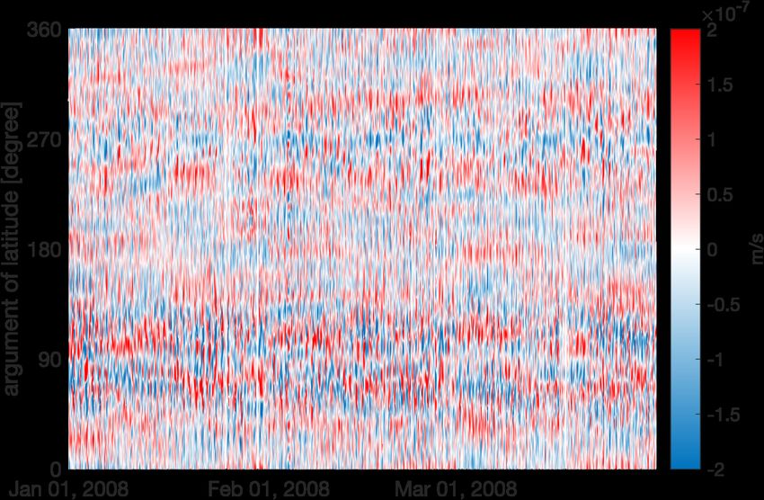
Remote Sens. 2021, 13, 1766                                                                                               3 of 23

                              Association of Geodesy (IAG). Within COST-G, monthly gravity field solutions of partici-
                              pating ACs and partner ACs are combined on solution [46] and normal equation levels [47],
                              in order to provide consolidated products with improved quality and higher robustness.
                              Since January 2021, LUH/IfE has been an official COST-G GRACE-FO AC and is contribut-
                              ing with the LUH-GRACE-FO-2020 solutions to the COST-G operational GRACE-FO time
                              series of monthly gravity fields [48].
                                   Here, we present and discuss the processing strategy of the LUH-GRACE-FO-2020
                              time series of monthly gravity field solutions. We give an overview on the underlying
                              theory (see Section 2.1), as well as review and summarize the corresponding mathematical
                              framework in a compact form (see Appendices A.1 and A.2).The processing strategy of
                              the LUH-GRACE-FO-2020 time series is summarized in Section 2.2. Utilized GRACE-
                              FO data products are listed in Section 2.3. In Section 3, the obtained monthly gravity
                              field solutions are evaluated by comparison to solutions of the GRACE-FO Science Data
                              System (SDS) and COST-G ACs. We compare the mean spectral noise level of the solutions
                              in terms of difference degree standard deviations (see Section 3.1). The spatial noise
                              level is assessed by analyzing residual equivalent water height (EWH) signal over the
                              oceans (see Section 3.1). To evaluate the signal content of the solutions, we compare the
                              annual and semi-annual EWH amplitudes of major river basins, and annual mass loss
                              trends in Greenland’s drainage basins (see Section 3.2). Finally, in Section 3.3, GRACE-FO
                              KBRR post-fit residuals are compared to those of the GRACE mission in frequency and
                              spatial domains.
                                   The presented results confirm that the outlined processing strategy is suited for ob-
                              taining monthly gravity field solutions with a quality competitive to that of the established
                              ACs. The noise level assessment points out processing strategy related differences among
                              the separate ACs, although the signal content is mostly not affected by these differences
                              and is very similar for all ACs. The carried-out comparison of GRACE and GRACE-FO
                              KBRR post-fit residuals highlights the overall improvement of the GRACE-FO K-Band
                              ranging system performance. Nevertheless, several common systematic effects can be
                              identified in GRACE and GRACE-FO post-fit residuals, e.g., higher noise related to shadow
                              transitions, or spikes at multiples of the orbital and daily frequencies.

                              2. Methods and Materials
                              2.1. Gravity Field Recovery as a Generalized Dynamic Orbit Determination
                                    The movement of an artificial satellite of the Earth is affected by the characteristics of
                              its surrounding environment. By implication, the position (absolute, relative) and velocity
                              coordinates—or the orbit of a satellite—contain information on a considerable number
                              of parameters that are primarily but not exclusively describing physical and geometrical
                              properties of the Earth. The time-variable gravity (TVG) is the main effect governing the
                              motion of a LEO satellite. Modeling of the satellite–environment interaction allows us
                              to derive the parameters describing Earth’s TVG in terms of the gravitational potential
                              V. The gravitational potential V at a location (λ, ϕ, r ) on or above the Earth’s surface can
                              be represented as a synthesis of normalized spherical harmonic coefficients C nm and Snm ,
                              e.g., [49,50]:
                                                        ∞             n    n
                                                GM⊕               R⊕
                                                       ∑                    ∑

                                           V=                                      C nm cos mλ + Snm sin mλ Pnm (sin ϕ)      (1)
                                                 r     n =0
                                                                   r        m =0

                              where λ, ϕ are the spherical longitude and latitude in an Earth-centered and Earth-fixed
                              frame, e.g., International Terrestrial Reference Frame (ITRF) [51]; r is the radial distance;
                              GM⊕ is the standard gravitational parameter of the Earth or the product of the universal
                              gravitational constant G and Earth’s mass M⊕ ; R⊕ is chosen as the semi-major axis of
                              the Earth’s ellipsoid; Pnm are normalized associated Legendre functions; and n, m are
                              degree and order of the spherical harmonic coefficients expansion. The objective of GFR—
                              and consequently of this work—is the estimation of the normalized spherical harmonic
                              coefficients C nm and Snm . A set of estimated coefficients until a specific maximum degree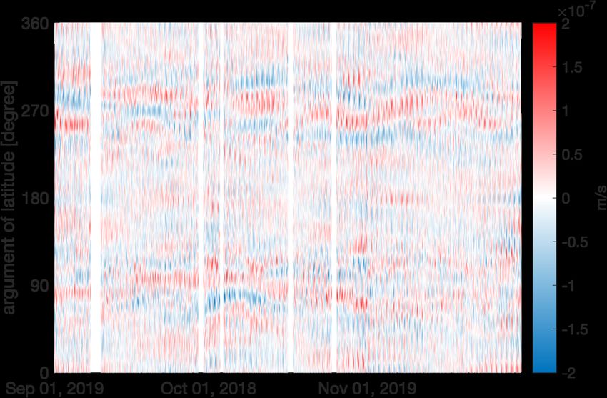
Remote Sens. 2021, 13, 1766                                                                                                4 of 23

                              nmax , including the constants GM⊕ and R⊕ , is referred to as a gravity field solution. In the
                              case of GRACE and GRACE-FO, the most common type of products are monthly gravity
                              field solutions.
                                    Powerful tools for the analysis of the satellite–environment interaction are the dynamic
                              and reduced dynamic orbit determination methods. These methods make use of orbit
                              modeling, numerical integration and parameter estimation to solve the satellite’s equation
                              of motion, e.g., [52,53]:
                                                                             GM⊕
                                                                      r̈ = − 3 r + r̈P                                      (2)
                                                                              r
                              where r and r̈ are satellite’s cartesian position and acceleration vectors in an inertial coordi-
                              nate frame, e.g., Geocentric Celestial Reference Frame (GCRF) [51]; the first added − GM    r3
                                                                                                                             ⊕
                                                                                                                               r
                              is the central body acceleration based on Newton’s law of universal gravitation and the
                              assumption that the satellite’s mass is negligible if compared to Earth’s mass M⊕ ; and
                              r̈P represents the sum of perturbing accelerations of gravitational and non-gravitational
                              nature. For the precise dynamic orbit determination of LEO satellites and for GFR as
                              applied in this work, the sum of perturbing accelerations can be formulated as follows:

                                                               8
                                                              ∑ r̈i
                                                                         gcrf        gcrf
                                                      r̈P =           + Ritrf ∇V + Rsrf         S r̈ng,srf + b                (3)
                                                              i =1
                                                                           r̈tvg                  r̈ng

                              where the summation ∑8i=1 r̈i considers separate gravitational effects of tidal and non-tidal
                              nature, as numbered (i) and described in Table 1. The acceleration r̈tvg is caused by Earth’s
                              TVG. Applying the Nabla operator ∇ = (∂/∂x ∂/∂y ∂/∂z)T to potential V results in the
                                                                                         gcrf
                              corresponding acceleration in ITRF. The rotation matrix Ritrf transforms the acceleration to
                              GCRF. The acceleration r̈ng is caused by non-gravitational effects such as atmospheric drag,
                              direct solar radiation pressure, Earth’s albedo and thermal emission. A bias vector b and
                              scale matrix S are needed for the calibration of the observed non-gravitational acceleration
                                                              gcrf
                              r̈ng,srf . The rotation matrix Rsrf formed from normalized quaternions transforms the
                              calibrated non-gravitational acceleration from the satellite body-fixed science reference
                              frame (SRF) to GCRF.

                              Table 1. Force/acceleration modeling standards of the LUH-GRACE-FO-2020 time series. d/o:
                              indicates the applied maximum degree/order of the spherical harmonic coefficients. Iterator i refers
                              to Equation (3).

                              i        Force/Acceleration                            Models and Parameters
                              -           Gravity field               GOCO06s (static: d/o 300, time-variable: d/o 200) [17]
                              1           Direct tides                Moon, Sun, Mercury–Saturn (DE430 ephemerides [54]);
                                                                               J2 effect considered for the Moon
                              2         Solid Earth tides                 Moon and Sun (d/o: 4); anelastic Earth [51];
                              3           Ocean tides                              FES2014b (d/o: 180) [19];
                                                                          361 minor waves based on admittance [55];
                              4        Relativistic effects                       IERS Conventions 2010 [51]
                              5       Solid earth pole tides                      IERS Conventions 2010 [51]
                              6         Ocean pole tides                IERS Conventions 2010/Desai (d/o: 180) [51,56]
                              7        Atmospheric tides                          AOD1B RL06 (d/o: 180) [21]
                              8            De-aliasing                            AOD1B RL06 (d/o: 180) [21]
                                                                               GRACE-C: ACT1B products [43];
                              -        Non-gravitational                    GRACE-D: alternative ACT products [57]

                                  The equation of motion is a vector form of an ordinary differential equation (ODE) of
                              second order. Since an ODE of order n can be reduced to n first order ODEs, the equation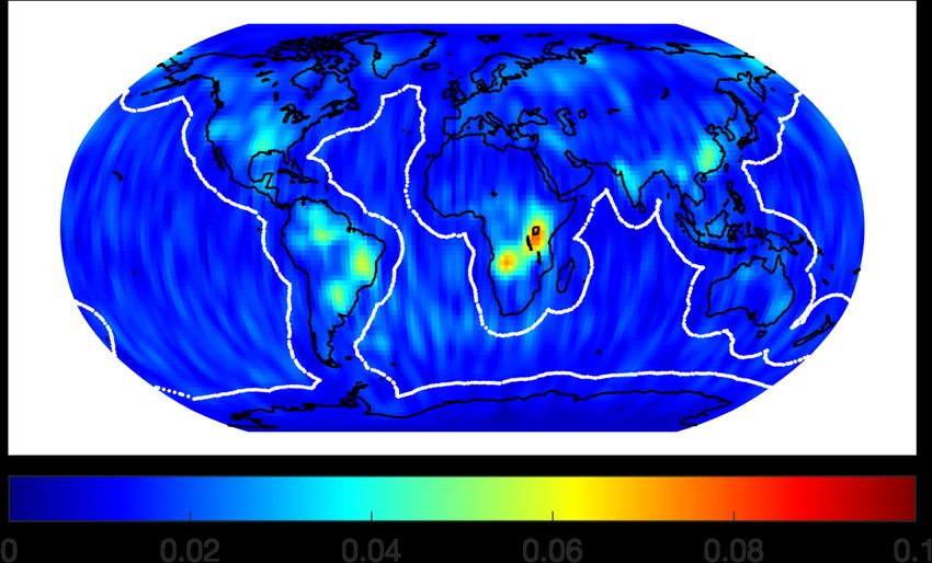
Remote Sens. 2021, 13, 1766 5 of 23
of motion is related to a satellite state y = (rT , ṙT )T containing the position vector r and
the velocity vector ṙ via the following two first order ODEs, e.g., [52,53]:
ṙ = v
GM⊕ (4)
v̇ = − r + r̈P .
r3
The integration of these ODEs results in a satellite state y. The six elements of the
initial state vector y0 = y(t0 ) at time t0 can be treated as integration constants. Due to
the complexity of the perturbing accelerations r̈P , the integration can not be performed
analytically, i.e., a satellite state at an arbitrary time t can not be obtained directly. Several
numerical integration methods can be used to achieve an approximative solution of satis-
factory quality. A dynamic intermediate orbit consisting of several states y at epochs t can
be obtained stepwise through the numerical integration of the two above-stated first-order
ODEs, as follows: Z t1 Z t2
y(t) = y0 + ẏ(t)dt + ẏ(t)dt + · · · (5)
t0 t1
y( t1 )
y( t2 )
where ẏ = (ṙT , v̇T )T combines the two first-order ODEs in a column vector. The inter-
mediate dynamic orbit as a series of satellite states (y0 , y(t1 ), y(t2 ), · · · ) is often referred
to as a dynamically modeled or numerically propagated orbit. Even when assuming the
best possible case for the integration constants in Equation (5), i.e., when the initial state is
known very accurately, the dynamically modeled orbit will deviate from a true orbit in the
course of time considerably. This is most of all due to uncertainties present in the models
describing separate effects of the perturbing acceleration r̈P . In addition, also the numerical
integration method, including specifics like the length and step size of the integration,
contributes to a deviation of the dynamically modeled orbit from a true orbit.
The concept of dynamic orbit determination is to adjust the dynamically modeled orbit
to observations. Speaking generally, optimal values for the initial state and other dynamic
parameters have to be found, so that the propagated orbit fits the observations in the
best possible way. When additionally empirical parameters are introduced as unknowns,
then the dynamic orbit determination approach becomes reduced-dynamic. Making use
of these additional parameters allows a better fit of the numerically propagated orbit
to observations. If the normalized spherical harmonic coefficients C nm and Snm are also
part of the to be estimated dynamic parameters, the dynamic or reduced-dynamic orbit
determination becomes a combined orbit determination and GFR.
The adjustment of the numerically propagated orbit to observations is usually accom-
plished by batch least squares adjustment. The linearized observation equations needed
for the estimation of unknown parameters in GFR from GRACE and GRACE-FO sensor
data can be summarized in the following simplified form:
n∼ ∂vec(rC ) n⊕ ∂vec(r )
C
vec(rC − rC ) = ∑ ∆q∼k + ∑ ∆q⊕k
k =1 ∂q∼k k =1 ∂q⊕k
n∼ n⊕ ∂vec(r )
∂vec(rD ) D
vec(rD − rD ) = ∑ ∆q∼k + ∑ ∆q⊕k .
k =1 ∂q ∼k k =1 ∂q ⊕k
n⊕
(6)
n∼ ∂ρ̇ ∂ρ̇
ρ̇ − ρ̇ ∑ ∆q∼k + ∑ ∆q⊕k
=
k =1 ∂q ∼k k =1 ∂q ⊕k
local global
On the left side of this equation, the reduced observation vectors (observed−computed)
can be found. These are formed as differences between the pseudo-observed orbit positions
of the two satellites rC , rD or measured KBRR ρ̇; and the dynamically modeled counterparts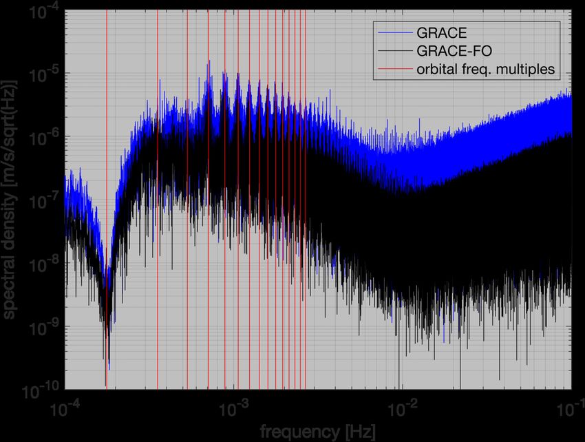
Remote Sens. 2021, 13, 1766                                                                                             6 of 23

                              rC , rD , ρ̇. Note that vec() is the vectorization operator, which converts a batch of orbit
                              position vectors to a column vector. The right side of the observation equations consists
                              of the partial derivatives of the dynamically modeled quantities with respect to (w.r.t.)
                              the unknown parameters q. It is very common to divide the unknown parameters into a
                              subset of local (∼) and global (⊕) parameters. The local parameter vector q∼ consists of
                              n∼ elements and the global parameter vector q⊕ is made up of n⊕ quantities, among them
                              the spherical harmonic coefficients of Earth’s gravitational potential. Since dynamic orbit
                              determination and GFR constitute a highly non-linear problem, the final parameters are
                              obtained as the sum of a priori parameters and the estimated correction vectors ∆q∼ and
                              ∆q⊕ in an iterative manner.
                                    For the sake of completeness, clarity and a more simple reproducibility, the mathemat-
                              ical framework of the gravity field parameter estimation is treated in detail in the appendix.
                              The appendix is divided into two parts: Appendix A.1 linear algebra and Appendix A.2
                              analysis. Appendix A.1 summarizes aspects of the parameter estimation, such as the
                              parameter pre-elimination, combination of normal matrices and post-fit residuals computa-
                              tion. Appendix A.2 covers topics such as the linearization of observation equations and the
                              formation of design matrices.

                              2.2. Processing Details
                                   For performance reasons, the processing consists of two main steps. In a first step,
                              an orbit pre-adjustment is performed without solving for the gravity field parameters.
                              Estimated arc parameters from the pre-adjustment are used as a priori values in a second
                              step, where the gravity field parameters are estimated along with the orbit in one iteration.
                              The main characteristics of this two-step approach are summarized in Table 2 and outlined
                              in detail below:

                              Table 2. Main specifics of the gravity field recovery two step approach. VCE: Variance Component
                              Estimation; σ: standard deviation; d/o: degree/order.

                                           Step 1                                       Orbit Pre-Adjustment
                                       arc length                                                  3h
                                   numerical integration                     modified Gauss-Jackson with 5 s step size
                                      observations                                    KBRR with 5 s sampling;
                                                                              kinematic positions with 30 s sampling
                                         weights                                    VCE per observation group
                                     local parameters                            initial state, accelerometer biases
                                    global parameters                                              no
                              constraints and regularization                                  not applied
                                           Step 2                         Orbit Adjustment and Gravity Field Recovery
                                       arc length                                           same as in step 1
                                   numerical integration                                    same as in step 1
                                      observations                                          same as in step 1
                                        weights                                       KBRR: σ = 2 × 10⁻⁷ m/s;
                                                                                 positions: orbit covariance matrix
                                       local parameters                           initial state, accelerometer biases
                                                                                     empirical KBRR parameters
                                    global parameters                           gravitational potential up to d/o 96;
                                                                                   full accelerometer scale matrix
                              constraints and regularization                                   not applied

                              1.   Orbit pre-adjustment
                                   •     Orbit modeling—Orbit arcs with a length of 3 h (approximately 2 revolutions),
                                         state transition and sensitivity matrices are simultaneously integrated in 5 s steps
                                         using a modified version of the Gauss–Jackson integration technique [58]. A
Remote Sens. 2021, 13, 1766 7 of 23
straightforward implementation of this efficient integration approach is described
in [14]. Forces of gravitational and non-gravitational nature affecting the motion
of the satellites are modeled according to the information given in Table 1. An
exception is made for the forces due to Earth’s gravity field. In order to speed up
the computation in this step, the gravity field is considered only until degree and
order 120. The force modeling implementations were evaluated in a software
comparison in the framework of COST-G. Implementations of all separate force
effects agree well with the implementations of the COST-G ACs. The differences
with regard to the implementations of other ACs are several orders of magnitude
below 10−10 m/s2 [59].
• Arc length—The 3 h arc length employed in our approach differs considerably
from the approaches of other ACs. The usual standard arc length employed by
other ACs for numerical integration and GFR from GRACE and GRACE-FO data
is 24 h. The aim of the rather short arc length is to allow a more precise orbit
fit to the pseudo-observed positions and KBRR measurements, as inaccuracies,
e.g., in force modeling, can be compensated by the frequent estimation of local arc
parameters. In contrast to the very common arc length of one day, no constrained
parameters, e.g., cycle per revolution accelerations, have to be co-estimated in
order to achieve an adequate orbit fit. Since a decrease of the arc length increases
the amount of arcs that can be processed independently, a considerable amount
of processing time can be saved if parallel computing is utilized.
• Observations—The reduced observation vectors are formed as differences be-
tween kinematic orbit positions or KBRR measurements and the corresponding
quantities obtained from the dynamically integrated orbit (see Equations (A10)
and (A12)). For KBRR measurements, the original 5 s sampling is kept. Kinematic
orbits from the Astronomical Institute of the University of Bern (AIUB) are down-
sampled to 30 s and used as pseudo observations. Due to the general prevailing
noisy character of kinematic orbits, compared to the rather smooth reduced-
dynamic orbits, a screening is performed. Epochs with a position difference
larger than 8 cm w.r.t. the reduced-dynamic GNV1B orbits are not considered
during parameter estimation.
• Weights—The partials of the numerically integrated orbit w.r.t. unknown param-
eters are used to set up the design matrices. Then, technique-specific normal
matrices are formed and combined. To set up the weight matrices, an initial
standard deviation of 0.2 µm/s for KBRR is used. For the pseudo-observed
position components, an initial standard deviation of 0.02 m is assumed. Vari-
ance component estimation, e.g., [60], is used to improve the technique-specific
weights after each iteration of the orbit determination.
• Parameters—Corrections to the initial state vectors and accelerometer bias param-
eters are estimated arc-wise based on least squares adjustment. Accelerometer
scale factors, accelerometer shear and rotation parameters needed for a full scale
matrix [23] are estimated monthly. For this purpose, the scale factors are fixed
to 1 and the accelerometer shear and rotation parameters to 0. The objective of
this step is not to obtain a best possible orbit fit, but rather to estimate appro-
priate initial values for the second step, therefore no empirical parameters are
co-estimated. A priori values of the unknowns are corrected iteratively until
convergence using the estimated corrections. A convergence is assumed when
the mean of absolute KBRR reduced observation differences of two consecutive
iterations is smaller than 0.1 µm/s .
• Outlier arcs—After the pre-adjustment of all monthly arcs, an inspection is per-
formed in order to detect spurious arcs that might disturb the GFR in the second
step. Kinematic empirical KBRR parameters [61] consisting of 90 min biases and
bias-rates, as well as 180 min periodic biases and bias-rates are fitted to each
KBRR reduced observation vector. The fitted signal is subtracted from the KBRRRemote Sens. 2021, 13, 1766 8 of 23
reduced observation vectors. Then, the root mean square (RMS) of this difference
is formed for each arc of a month. Finally, a sigma-based screening is applied
to the time series of these quantities. Arcs outside the 3 sigma bounds are not
considered in the further processing.
2. Orbit adjustment and gravity field recovery
• Orbit modeling—Initial states and accelerometer biases from the pre-adjustment
are used as new a priori values for the dynamic orbit modeling and computation
of the state and parameter sensitivity matrices. Forces are modeled according to
the description given in Table 1. Method specifics for the numerical integration
are unchanged from step 1.
• Observations—The formation of reduced observation vectors is consistent with
the procedure in the pre-adjustment.
• Weights—A standard deviation of 0.2 µm/s is used to set up the KBRR weight
matrices. In case of kinematic positions, the inertial orbit covariance informa-
tion is used to form diagonal weight matrices. We divide the elements of the
kinematic positions weight matrices by an empirical factor of 25. Without this
downweighting of the kinematic orbit covariance information, the quality of
obtained solutions is unsatisfactory. A downweighting of GNSS-based obser-
vations w.r.t. KBRR measurements is an issue already known from the GRACE
processing, e.g., [6,8], and deserves further attention in the future.
• Parameters—The local parameters, i.e., initial states and accelerometer biases, are
re-estimated in this step. In addition, the set of local parameters is extended by
kinematic empirical KBRR parameters to absorb effects due to the possible mis-
modeling of perturbing accelerations. The set of kinematic empirical parameters
is consistent with the definition utilized previously in the outlier arc detection.
The normalized spherical harmonic coefficients of the monthly Earth’s gravita-
tional potential up to degree and order 96, as well as accelerometer scale factors,
rotation and shear parameters, are introduced as global unknowns. The contribu-
tion of an arc to the set of global parameters is estimated after pre-elimination
of the local parameters from the system of normal equations. The contributions
of all 3 h arcs of a month are accumulated in order to obtain the final global
parameters (see Equation (A3)).
• Outlier screening—KBRR post-fit residuals are computed and a visual screening is
performed in time and frequency domains (see Section 3.3). In case of additional
outliers, the second step is repeated.
2.3. GRACE-FO Sensor Data and Products
For the computation of the gravity field solutions presented in this study, GRACE-FO
Level-1B data products are used [43], which are generated by the SDS. The data products
can be obtained from NASA’s Physical Oceanography Distributed Active Archive Center
(PO.DAAC) [62] and from GFZ’s Information System and Data Center (ISDC) [63]. The
following Level-1B data products are used in this work:
• KBR1B: biased K-band ranges, as well as their first and second time derivatives
K-band range-rates and K-band range-accelerations given in 5 s sampling. KBRR
measurements are used as the main observations in the estimation process. The light
time correction and antenna center offset correction as given in the KBR1B product
are applied.
• GNV1B: main data in these products are 1 s satellite positions and velocities in ITRF
obtained from a reduced-dynamic orbit determination approach. In this work, the po-
sitions are used for modeling satellite accelerations caused by different forces (see
Table 1). Instead of evaluating the accelerations at intermediate positions during every
iteration of orbit determination, a major part of the accelerations is pre-computed
using the precise GNV1B orbits. Only the acceleration caused by the Earth’s gravita-Remote Sens. 2021, 13, 1766 9 of 23
tional potential is evaluated at every intermediate position during orbit determination
and GFR.
• SCA1B: 1 s normalized quaternions describing the rotation between SRF and GCRF.
Since the numerical orbit propagation is accomplished in an inertial frame, the quater-
nions are needed for transforming calibrated non-gravitational accelerations to GCRF
(see Equation (3)).
• ACT1B: main data in these products are 1 s linear accelerometer measurements given
in SRF. The measurements represent the sum of acceleration variations caused by
non-gravitational effects. Accelerometer calibration parameters have to be estimated
during orbit determination and GFR. The ACT1B products replace ACC1B products
that were formerly used for GFR from GRACE data. The main feature of ACT1B
is a so-called transplantation of GRACE-C accelerometer measurements to satellite
GRACE-D. The necessity for this transplantation [24] arises because of a severe
degradation of GRACE-D measurements, e.g., [40]. With the exception of June 2018,
only GRACE-C ACT1B products are used in this work.
In addition to the listed products, the following GRACE-FO data products are utilized:
• Alternative ACT products: For GRACE-D, for all months except June 2018, alternative
ACT products [57] from the Institute of Geodesy at Graz University of Technology are
used instead of the official ACT1B products.
• AIUB kinematic orbits: These kinematic orbits are produced at the Astronomical Insti-
tute at University of Bern. Processing details are summarized in [64]. The kinematic
orbits do not contain any information from dynamic models. The positions are treated
as pseudo-observations during parameter estimation. In addition to the positions, co-
factor matrices are also available. These matrices are used to form the corresponding
weight matrices.
3. Results and Evaluation
To evaluate the quality of the computed monthly gravity field solutions, the LUH-
GRACE-FO-2020 time series is compared to solutions of the SDS and COST-G ACs. In
Section 3.1, the noise level of the solutions is assessed and compared in spectral as well as
spatial domains. Annual and semi-annual EWH amplitudes of river basins and annual
mass loss trends in Greenland’s drainage basins are compared in Section 3.2. Typical
GRACE-FO and GRACE KBRR post-fit residuals are shown and compared in Section 3.3.
Note that because of the so far short GRACE-FO operation time, the below presented
comparisons constitute only a very preliminary image. The LUH solutions are compared
to the following publicly available solutions:
• CSR Release 06 (GFO) from the Center for Space Research at University of Texas,
Austin [65,66]
• GFZ Release 06 (GFO) from the German Research Centre for Geosciences in Pots-
dam [67,68]
• JPL Release 06 (GFO) from the Jet Propulsion Laboratory in Pasadena [5,69]
• ITSG-Grace_op from the Institute of Geodesy at Graz University of Technology [7,70]
• AIUB-GRACE-FO_ op from the Astronomical Institute at the University of Bern [71]
All these solutions are available on the website of the International Centre for Global
Earth Models (ICGEM) [72]. The regarded solutions allow a fair comparison, since the
processing is based on variants of the generalized dynamic orbit determination with
variational equations. In addition, all compared solutions are unconstrained, i.e., computed
without applying regularizations.
3.1. Noise Level
First, the overall noise levels of the solutions are compared in the spectral domain in
terms of mean difference degree standard deviations (DDSDs) with regard to a reference
model. Since in general, the normalized spherical harmonic coefficients of a gravity fieldRemote Sens. 2021, 13, 1766 10 of 23
solution may be scaled with different standard gravitational parameters of the Earth GM⊕
and Earth reference radii R⊕ , solutions of all ACs are re-scaled to the standard values from
the IERS Conventions 2010 [51]. One common reference model is computed as the mean
of all monthly GRACE-FO solutions available until now (June 2018 until December 2020).
Before computing the reference model, the C20 and C30 coefficients of all solutions are
replaced, with more accurate values obtained from satellite laser ranging (SLR) [73,74]. The
reference model is then subtracted from all solutions before computing monthly DDSDs.
Note that the DDSDs of the low degree coefficients are dominated by signal (approximately
until degrees 20–30), while higher degrees are dominated by noise.
The averaged DDSDs are illustrated in Figure 1. A high level of consistency can be
observed for the low degree coefficients that are of major importance for mass change
estimations due to a large signal content. Larger differences are observed for degree
2, among which the LUH and AIUB solutions have the smallest DDSDs. The smaller
DDSDs are primarily caused by less noisy C20 coefficients, meaning that, in general, the
C20 coefficients are closer to the more precise SLR coefficients. Since the GRACE-FO C20
coefficients are usually replaced with SLR coefficients, this smaller noise is not of great
relevance for the estimation of mass variations. Starting at around degree 12, the different
processing strategies of the ACs are causing noticeable deviations of the DDSDs. The
LUH solutions slightly outperform the GFZ solutions and have a noise level similar to
that of the JPL solutions along major parts of the spectrum. AIUB’s solutions based on the
celestial mechanics approach, e.g., [75], have slightly less noise in the coefficients between
degrees 30 and 70, compared to GFZ, JPL and LUH. The ITSG solutions that incorporate an
advanced stochastic modeling and additional tidal estimates, e.g., [7,76], have the overall
smallest noise level. Moreover, the solutions from CSR suppress noise better than most
ACs. This might be due to the fact that in CSR’s GFR strategy, the local parameters are
estimated beforehand. During the estimation of spherical harmonic coefficients of Earth’s
gravitational field, the local parameters are not re-estimated [4].
difference degree standard deviation [-]
10 -9
CSR
GFZ
JPL
ITSG
10 -10 AIUB
LUH
-11
10
0 20 40 60 80
degree [-]
Figure 1. Mean difference degree standard deviations of monthly gravity field solutions from June
2018 until December 2020 with regard to a mean field. Mean field is the average of solutions of all
ACs. C20 coefficients are zero tide in all solutions.
The noise level of the solutions in the spatial domain can be assessed by analyzing
residual mass variations in suited regions. A suited region is defined as an area where
only relatively small mass variations are present, e.g., oceans. For comparison of the
noise characteristics in the spatial domain, the normalized spherical harmonic coefficients
are converted to 2◦ × 2◦ global gridded mass variations in terms of EWHs, e.g., [77,78].
The EWH values are computed with regard to the mean model that was already used forRemote Sens. 2021, 13, 1766 11 of 23
the mean DDSDs. A Gaussian filter [77] with an averaging radius of 400 km is applied
in order to mitigate the typical meridional striping. A model consisting of a bias, trend,
annual and semi-annual variation is fitted to each grid cell of the EWH time series to
absorb time-variable signal. After reduction of this simplified model, the residual signal
over the oceans is rather homogenous, while several regions on land show the presence of
unabsorbed hydrological signal, e.g., in Africa and South America (see Figure 2). Since
solely the areas over oceans are of interest, only values inside an ocean mask are considered.
The comparison of the monthly RMS noise over the oceans can be seen in Figure 2. The
monthly RMS noise over the ocean values highly correlate with the earlier presented
DDSDs. Particularly striking are two ocean noise RMS values in the ITSG time series,
i.e., October 2018 and February 2019, where the ITSG values are slightly larger, compared
to the very small noise level during other months. This can be explained by larger sensor
data gaps during these months. In contrast to ITSG, the other ACs utilize additional sensor
data from neighboring months in order to stabilize their solutions during these months.
The ACs’ mean RMS values of the residual signal (October 2018 and February 2019 not
considered) are: CSR: 1.45 cm, GFZ: 2.26 cm, JPL: 1.68 cm, ITSG: 1.20 cm, AIUB: 1.57 cm
and LUH: 1.65 cm.
3.5
CSR
GFZ
JPL
3 ITSG
AIUB
LUH
2.5
EWH RMS [cm]
2
1.5
1
0.5
2018-07 2019-01 2019-07 2020-01 2020-07
date
Figure 2. Left panel: Residual EWH signal of the LUH solutions after subtracting a model consisting of bias, trend, annual
and semi-annual variations. White lines represent the applied ocean mask. Units of the color bar: m. Right panel: RMS of
residual EWH signal over the oceans. C20 and C30 coefficients are replaced with SLR values. Gaussian filter with a 400 km
averaging radius applied.
3.2. Signal Content
Annual and semi-annual amplitudes in terms of mean EWHs of about 180 major river
basins are compared. The geographical boundaries of the river basins were taken from the
Total Runoff Integrating Pathways (TRIP) product [79,80]. The global EWHs are computed
according to the same procedure earlier used for the assessment of the spatial noise. Note
that the C20 as well as C30 coefficients were replaced with SLR-derived values. To each
2◦ × 2◦ cell, a model consisting of a bias, trend, annual and semi-annual variation was
fitted. Then, the mean annual and semi-annual EWH amplitudes in the boundaries of each
river basin region were formed (see Figure 3a,b). For each river basin amplitude, an error
bar is shown. These error bars represent −/ + 3 sigma w.r.t. the mean amplitude of all ACs.
The amplitudes are sorted in decreasing order w.r.t. ITSG amplitudes. It can be seen that
none of the annual or semi-annual amplitudes are outside the error bars. This indicates a
good agreement of the signal contained in the solutions of the ACs.Remote Sens. 2021, 13, 1766 12 of 23
0.25 0.25
ITSG
CSR
0.2 0.2 GFZ
JPL
AIUB
0.15 0.15
amplitude [m]
amplitude [m]
LUH
-/+ 3 sigma
0.1 0.1
0.05 0.05
0 0
-0.05 -0.05
20 40 60 80 100 120 140 160 180 20 40 60 80 100 120 140 160 180
basin number basin number
(a) Annual amplitudes (b) Semi-annual amplitudes
-15
NO
-20
-25 NW
trend [Gt/yr]
NE
-30
CW
-35
SW SE
-40
-45
NW CW SW SE NE NO
drainage basin
(d) Greenland drainage basins
(c) Annual mass trend
Figure 3. Upper panels: Annual (a) and semi-annual (b) river basin amplitudes in terms of mean EWH. 3-sigma-limits are
with regard to the mean amplitudes of all ACs. The river basin numbers in (a,b) do not correspond to each other. Bottom
panels: Annual mass change trend (c) in six regions of Greenland (d). C20 and C30 are replaced with SLR values. Gaussian
filter with a 400 km averaging radius applied. Presented results are based on data from June 2018 until December 2020.
Next, mass loss trends in six drainage basins of Greenland (see Figure 3d) are com-
pared. The definitions of the drainage basin region boundaries were taken from the Ice
Sheet Mass Balance Inter-comparison Exercise (IMBIE) dataset [81]. The mean EWH trends
are converted to mean mass trends expressed in Giga tons per year (Gt/yr). Degree 1
coefficients were not added. Note that the mass trends are neither corrected for glacial
isostatic adjustment nor the leakage effect. The obtained annual mass loss trends are
illustrated in Figure 3c. The trend estimates of all ACs show a high level of agreement for
all six regions of Greenland. The highest discrepancy in the trend amplitudes of about
3.35 Gt/yr can be found in the SW basin. On average, the maximum discrepancy is about
2 Gt/yr.
3.3. KBRR Post-Fit Residuals
In this section, three months of exemplary GRACE KBRR post-fit residuals (January
2008 until March 2008) are compared to three months of exemplary GRACE-FO KBRR
post-fit residuals (September 2019 until November 2019). The utilized GRACE gravityRemote Sens. 2021, 13, 1766 13 of 23
field solutions were computed according to the processing strategy summarized in [13,14].
The GRACE-FO KBRR post-fit residuals are routinely examined and are an important
component of the outlier screening strategy of the LUH-GRACE-FO-2020 solutions (see
Section 2.2). The KBRR post-fit residuals are computed according to Equation (A7). It
should be emphasized that for GRACE-FO, a revised processing is applied. The most
important differences concern the utilized background models for the ocean tides (GRACE:
EOT11a [18], GRACE-FO: FES2014b) and non-tidal short-term variations of the oceans and
the atmosphere (GRACE: AOD1B RL05 [20], GRACE-FO: AOD1B RL06). Moreover, in the
case of GRACE-FO, a full accelerometer scale matrix is estimated.
In the following, we inspect spatial and temporal characteristics of KBRR post-fit
residuals in time-argument-of-latitude (TAL) diagrams, the argument of latitude being the
geocentric angle in the orbital plane between the ascending node and the position of the
spacecraft. In TAL diagrams, systematic effects that depend on the orbital configuration
(e.g., the position and orientation of the satellites with regard to Earth and Sun) tend
to stand out as distinct and coherent structures. We focus on two bands of band-pass
filtered KBRR post-fit residuals. The first band (A) extends from 0.6 mHz to 5 mHz. This is
above the frequencies where empirical parameters directly absorb errors and unmodeled
signal contributions. In band A, we expect the geophysical aliasing of unmodeled tidal
and non-tidal mass variations, as well as slowly drifting instrument systematics as main
contributors to residuals. The second band (B) extends from 5 mHz to 20 mHz. In this band,
the influence of mass variations to residuals is fading out due to the limited sensitivity of
the GRACE-FO constellation, however, it is a band that is well suited to detect systematics
due to changes in the orbital configuration and/or the instrument operation.
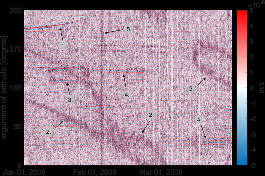
The TAL diagrams of these two bands can be seen in Figure 4. The post-fit residuals
in the 0.6 to 5 mHz frequency band differ in their intensity. The GRACE-FO residuals are
distinctively smaller. Several geographical patterns of different amplitudes and periodici-
ties are visible in this band. Some of these features are, for example, daily patterns related
to the Earth rotation and patterns with a period of approximately 30 days, which are more
distinct around degrees 90 and 270, i.e., at the poles. The features in the 0.6 to 5 mHz
frequency band might be caused by uncertainties in models of rapid tidal and non-tidal
mass variations. The modeling of the rapid tidal and non-tidal mass variations is still one of
the major error contributors in GFR. The smaller GRACE-FO residuals in this band can be
explained to a certain extent by earlier mentioned updates in background force modeling.
The appearance of the residuals in the 5 to 20 mHz frequency band differs consider-
ably for the two missions. Several systematics are present in GRACE post-fit residuals,
e.g., during the entering and exit phase into and from the penumbra region (1.) [82],
frequency-related KBR system signal-to-noise ratio drops (2.) [83,84], baffle-related KBR
system signal-to-noise ratio drops (3.) [83,84], systematics possibly related to the star cam-
era assembly (4.). In addition, a vertical line can be seen (5.) that is caused by bad sensor
data in the involved arcs. In the computation of the LUH-GRACE-FO-2020 solutions, such
artifacts are detected and removed during outlier detection. Except the patterns related
to the entering and exit phase into and from the penumbra region (1.), the GRACE-FO
residuals in the 5 to 20 mHz frequency band do not explicitly reveal any of the previously
listed systematic errors. Nevertheless, very slight systematics which manifest as horizontal
lines are recognizable at approximately 90 and 270 degrees (2.). These horizontal lines
correlate with systematics in the 0.6 to 5 mHz frequency band.
Noticeable is the overall amplitude difference of the post-fit residuals. The corre-
sponding unfiltered RMS during the three examined GRACE-FO months (8.0 × 10⁻⁸ m/s)
is approximately three times smaller than the RMS during the three GRACE months
(3.0 × 10⁻⁷ m/s). These findings are consistent with the results presented in [40].Remote Sens. 2021, 13, 1766 14 of 23
(a) Band A: GRACE (b) Band A: GRACE-FO
(c) Band B: GRACE (d) Band B: GRACE-FO
Figure 4. Time-Argument-of-Latitude (TAL) diagrams illustrating frequency filtered exemplary GRACE (left) and GRACE-
FO (right) KBRR post-fit residuals. Upper panels: residuals in the 0.6 to 5 mHz frequency band; bottom panels: residuals in
the 5 to 20 mHz frequency band. See text for definition of highlighted patterns.
Figure 5 illustrates the power spectral density (PSD) of the KBRR post-fit residuals
in the frequency band from 10−4 to 10−1 Hz. GRACE-FO amplitudes are distinctively
smaller along the whole spectrum, compared to GRACE. Very prominent is the difference
in the frequency range between 10−2 and 10−1 Hz. The smaller GRACE-FO amplitudes
in this frequency band are related to the lower noise level of the GRACE-FO KBR system,
e.g., [40]. Highlighted with red vertical lines are the first 15 orbital frequency multiples
(1 cycle per revolution (cpr) to 15 cpr). The PSD of the residuals is dominated by spikes
located at orbital frequency multiples. As expected from Figure 4a,b, spikes are also present
at multiples of the daily frequency, although they only become visible when an appropriate
zooming is applied to the PSD figure. In contrast, the smaller residuals around 1 cpr
can be regarded as exceptions, since they are absorbed by the co-estimation of arc-wise
empirical KBRR parameters (see Section 2.2). The estimation of additional empirical KBRR
parameters in order to absorb further frequencies is currently under investigation.Remote Sens. 2021, 13, 1766 15 of 23
Figure 5. Power spectral density of the KBRR post-fit residuals in the frequency band from 10−4 to
10−1 Hz. First 15 multiples of the orbital frequency are highlighted.
4. Conclusions
The Institute of Geodesy at Leibniz University Hannover produces unconstrained
GRACE-FO monthly gravity field solutions. The solutions are computed with the MATLAB-
based GRACE-SIGMA software package recently developed at Leibniz University Han-
nover. The solutions are obtained from GRACE-FO Level-1B products, alternative ac-
celerometer products produced at Graz University of Technology, and kinematic orbits
from the Astronomical Institute at University of Bern. The regularly updated time series
named LUH-GRACE-FO-2020 is accessible on the website of the International Centre for
Global Earth Models [85] and in LUH’s research data repository [86].
The quality of the solutions is competitive with those of the GRACE-FO Science
Data System and Combination Service for Time-variable Gravity Fields analysis centers.
While the spectral and spatial noise levels of the separate analysis centers slightly differ,
the signal content of the solutions is very similar among all analysis centers. The C20 and
C30 coefficients were excluded from the comparison of the signal content and therefore
deserve further attention in the future. The GRACE-FO K-band range-rate (KBRR) post-fit
residuals are about three times smaller, compared to GRACE. Most pronounced systematics
in GRACE-FO KBRR post-fit residuals are related to the entering and exit phase into and
from the penumbra region. The power spectral density of the post-fit residuals is mainly
dominated by spikes located at multiples of orbital frequency. The analysis and further
understanding of the systematics in the post-fit residuals are important for identifying
factors that limit the quality of gravity field recovery.
Author Contributions: Conceptualization, I.K. and J.F.; methodology, I.K.; software, I.K. and M.D.;
validation, I.K. and J.F.; investigation, I.K.; data curation, I.K. and A.S.; writing—original draft
preparation, I.K.; writing—review and editing, I.K., M.D., J.F. and A.S.; visualization, I.K.; supervision,
J.F. and A.S.; project administration, J.F.; funding acquisition, J.F. All authors have read and agreed to
the published version of the manuscript.
Funding: This research received funding from the German federal state of Lower Saxony.
Data Availability Statement: The monthly gravity field solutions presented in this study are
openly available on ICGEM at http://icgem.gfz-potsdam.de/series/10.25835/0062546, accessedRemote Sens. 2021, 13, 1766 16 of 23
on 24 March 2021 [85]; and in the LUH Research Data Repository at https://data.uni-hannover.de/
dataset/luh-grace-fo-2020, accessed on 24 March 2021 [86].
Acknowledgments: We would like to thank the German Space Operations Center (GSOC) of the
German Aerospace Center (DLR) for providing continuously and nearly 100% of the raw telemetry
data of the twin GRACE-FO satellites. Majid Naeimi is acknowledged for developing the initial
version of GRACE-SIGMA. The colleagues from the Combination Service for Time-variable Gravity
Fields (COST-G) are acknowledged. The COST-G meetings helped us to improve our gravity
field recovery strategy. The International Space Science Institute (ISSI) in Bern/Switzerland is
acknowledged for hosting the COST-G team meetings in 2019, 2020 and 2021. Participation in
these meetings was financially supported by ISSI. We are thankful for the valuable comments of the
anonymous reviewers. The publication of this article was funded by the Open Access Fund of the
Leibniz Universität Hannover.
Conflicts of Interest: The authors declare no conflict of interest. The funders had no role in the design
of the study; in the collection, analyses, or interpretation of data; in the writing of the manuscript,
or in the decision to publish the results.
Abbreviations
The following abbreviations are used repeatedly in this manuscript:
AC Analysis Center
AIUB Astronomical Institute, University of Bern
COST-G COmbination Service for Time-variable Gravity fields
DDSD Difference Degree Standard Deviation
EWH Equivalent Water Height
GCRF Geocentric Celestial Reference Frame
GFR Gravity Field Recovery
GFZ GeoForschungsZentrum
(GFZ German Research Centre for Geosciences)
GNSS Global Navigation Satellite Systems
GRACE Gravity Recovery And Climate Experiment
GRACE-FO GRACE Follow-On
GRACE-SIGMA GRACE-Satellite orbit Integrator and Gravity field analysis in MAtlab
ITRF International Terrestrial Reference Frame
ITSG Institute for Theoretical and Satellite Geodesy
(now: Institute of Geodesy, Graz University of Technology)
JPL Jet Propulsion Laboratory
KBR K-Band Ranging
KBRR K-Band Range-Rate
LEO Low Earth Orbit
LUH Leibniz University Hannover
ODE Ordinary Differential Equation
PSD Power Spectral Density
RMS Root Mean Square
SDS (GRACE-FO) Science Data System
SLR Satellite Laser Ranging
SRF Science Reference Frame
TAL Time-Argument-of-Latitude
TVG Time-Variable Gravity
Appendix A
Appendix A.1. GFR Parameter Estimation: Linear Algebra
One of the most important parts of orbit determination and gravity field recovery
is parameter estimation. According to weighted least squares adjustment, the parameter
vector x̂ containing a set of unknowns can be obtained as follows, e.g., [87,88]:Remote Sens. 2021, 13, 1766 17 of 23
x̂ = (AT PA)−1 AT Pl
(A1)
= N−1 b
where A is the design matrix; P is the weight matrix; l is the observation vector; N is the
normal matrix; b the right hand side vector.
Because of the non-linearity of the orbit determination, approximate values of the
unknowns x0 are introduced and corresponding corrections ∆x̂ are estimated iteratively,
so that the parameter vector is defined as x̂ = x0 + ∆x̂. The presence of different types of
unknowns, i.e., local parameters such as the initial states; and global parameters like the
spherical harmonic coefficients of a gravity field solution, allows one to divide the parame-
ter correction vector into two parts: ∆x̂ = (∆x̂T∼ , ∆x̂T⊕ )T , where local and global parameters
are denoted with the subscripts ∼ and ⊕, respectively. In case of a set of arcs i = 1, 2, · · · , j,
the parameter correction vector can be extended to ∆x̂ = (∆x̂T∼1 , ∆x̂T∼2 , · · · , ∆x̂T∼ j , ∆x̂T⊕ )T .
Applying this separation of parameters to Equation (A1) leads to the below stated system
of normal equations that has to be solved, e.g., [60]:
N∼1 0 ··· 0 N∼⊕1 ∆x̂∼1 b∼1
∆x̂∼2 b∼2
0
N∼2 · · · 0 N∼⊕2
. . . .
.. .. .. .. .. ... = ...
. . (A2)
0 0 · · · N N ∼⊕ j ∆x̂∼ j b∼ j
∼j
NT∼⊕1 NT∼⊕2 · · · NT∼⊕ j N⊕ ∆x̂⊕ b⊕
The inversion of this system of normal equations according to Equation (A1) can
become heavily memory intensive and unsolvable. However, the final estimate of the global
parameter corrections ∆x̂⊕ can be obtained after pre-elimination of all local parameter
corrections, e.g., [60]:
j
∆x̂⊕ = ∑ ∆x̂⊕i , (A3)
i =1
where
−1
∆x̂⊕i = N⊕i − N∼⊕i T N−
∼i
1
N ∼⊕ i b ⊕ i − NT
∼⊕ i N −1
∼i b ∼ i . (A4)
KBRR observations have to be combined with GNSS tracking data, e.g., kinematic
orbits, in order to obtain a gravity field solution of satisfactory quality. The normal matrices
N∼i , N⊕i , N∼⊕i and the right hand side vectors b∼i , b⊕i can be formulated as technique-
specific weighted superimpositions of observations, e.g., [89]:
AT∼Ci PCi A∼Ci AT∼Di PDi A∼Di AT∼Ki PK A∼Ki
N∼ i = + +
N∼⊕i = AT∼Ci PCi A⊕Ci + AT∼Di PDi A⊕Di + AT∼Ki PK A⊕Ki
N⊕ i = AT⊕Ci PCi A⊕Ci + AT⊕Di PDi A⊕Di + AT⊕Ki PK A⊕Ki
(A5)
AT∼Ci PCi ∆lCi AT∼Di PDi ∆lDi AT∼Ki PK ∆lKi
b∼ i = + +
AT⊕Ci PCi ∆lCi AT⊕Di PDi ∆lDi AT⊕Ki PK ∆lKi
b⊕ i = + +
GNSS C GNSS D KBRR
where the contribution of satellite-specific positions is denoted with the subscripts C, D
and the contribution of KBRR with the subscript K; the vectors ∆lCi , ∆lDi and ∆lKi are
reduced observation vectors; these vectors as well as the design matrices A∼Ci , A∼Di , A∼Ki ,
A⊕Ci , A⊕Di and A⊕Ki are defined in Appendix A.2. PCi , PDi and PK are the weight matrices
representing the stochastic model of the observations. From the subscripts of the weightYou can also read