The impact of online machine-learning methods on long-term investment decisions and generator utilization in electricity markets

Page created by Jerome Fletcher
 
CONTINUE READING
The impact of online machine-learning methods on long-term investment decisions and generator utilization in electricity markets
The impact of online machine-learning methods on long-term investment
                                                       decisions and generator utilization in electricity markets

                                                                         Alexander J. M. Kell, A. Stephen McGough, Matthew Forshaw
                                                                       School of Computing, Newcastle University, Newcastle upon Tyne, United Kingdom
arXiv:2103.04327v1 [econ.EM] 7 Mar 2021

                                          Abstract
                                             Electricity supply must be matched with demand at all times. This helps reduce the chances of issues such as
                                          load frequency control and the chances of electricity blackouts. To gain a better understanding of the load that is
                                          likely to be required over the next 24 hours, estimations under uncertainty are needed. This is especially difficult in a
                                          decentralized electricity market with many micro-producers which are not under central control.
                                             In this paper, we investigate the impact of eleven offline learning and five online learning algorithms to predict the
                                          electricity demand profile over the next 24 hours. We achieve this through integration within the long-term agent-
                                          based model, ElecSim. Through the prediction of electricity demand profile over the next 24 hours, we can simulate
                                          the predictions made for a day-ahead market. Once we have made these predictions, we sample from the residual
                                          distributions and perturb the electricity market demand using the simulation, ElecSim. This enables us to understand
                                          the impact of errors on the long-term dynamics of a decentralized electricity market.
                                             We show we can reduce the mean absolute error by 30% using an online algorithm when compared to the best
                                          offline algorithm, whilst reducing the required tendered national grid reserve required. This reduction in national
                                          grid reserves leads to savings in costs and emissions. We also show that large errors in prediction accuracy have a
                                          disproportionate error on investments made over a 17-year time frame, as well as electricity mix.
                                          Keywords: Online learning, Machine learning, Market investment, Climate Change, Machine Learning

                                          1. Introduction                                                           Typically, peaker plants, such as reciprocal gas en-
                                                                                                                 gines, are used to fill fluctuations in demand that had
                                             The integration of higher proportions of intermittent               not been previously planned for. Peaker plants meet the
                                          renewable energy sources (IRES) in the electricity grid                peaks in demand when other cheaper options are at full
                                          will mean that the forecasting of electricity supply and               capacity. Current peaker plants are expensive to run and
                                          demand will become increasingly challenging 1 . Exam-                  have higher greenhouse gas emissions than their non-
                                          ples of IRES are solar panels and wind turbines. These                 peaker counterparts. Whilst peaker plants are also dis-
                                          fluctuate in terms of power output based on localized                  patchable plants, not all dispatchable plants are peaker
                                          wind speed and solar irradiance. As supply must meet                   plants. For example coal, which is a dispatchable plant,
                                          demand at all times and the fact that IRES are less pre-               is run as a base load plant, due to its inability to deal
                                          dictable than dispatchable energy sources such as coal                 with fluctuating conditions.
                                          and combined-cycle gas turbines (CCGTs), extra atten-
                                          tion must be made in predicting future demand if we                       To reduce reliance on peaker plants, it is helpful to
                                          wish to keep, or reduce, the current frequency of black-               know how much electricity demand there will be in the
                                          outs [1]. A dispatchable source is one that can be turned              future so that more efficient plants can be used to meet
                                          on and off by human control and is able to adjust output               this expected demand. This is so that these more effi-
                                          just in time at a moment convenient for the grid.                      cient plants can be brought up to speed at a time suitable
                                                                                                                 to match the demand. Forecasting a day into the future
                                                                                                                 is especially useful in decentralized electricity markets
                                               Email address: a.kell2@newcastle.ac.uk (Alexander J. M.
                                          Kell)
                                                                                                                 which have day-ahead markets. Decentralized electric-
                                             1 Matching of supply and demand will be referenced as demand        ity markets are ones where electricity is provided by
                                          from this point onwards for brevity.                                   multiple generation companies, as opposed to a cen-
                                          Preprint submitted to Sustainable Computing: Informatics and Systems                                                March 9, 2021
The impact of online machine-learning methods on long-term investment decisions and generator utilization in electricity markets
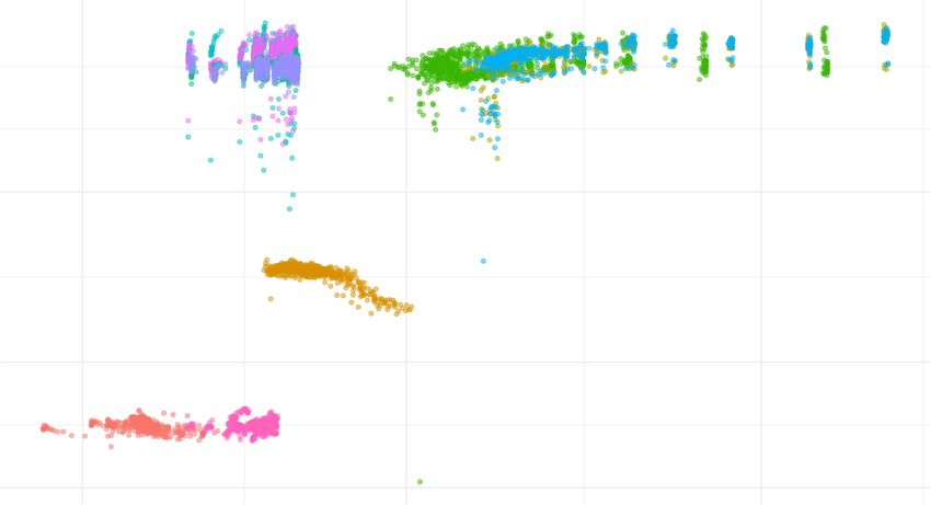
tralized source, such as a government. To aid in this            ilar load profiles due to the reduction in industrial elec-
prediction, machine learning and statistical techniques          tricity use and an increase in domestic use. This enables
have been used to accurately predict demand based on             an algorithm to become good at a specific subset of the
several different factors and data sources [2], such as          data which share similar patterns, as opposed to having
weather [3], day of the week [4] and holidays [5].               to generalize to all of the data. Examples of the algo-
   Various studies have looked at predicting electricity         rithms used are linear regression, lasso regression, ran-
demand at various horizons, such as short-term [6] and           dom forests, support vector regression, multilayer per-
long-term studies [7]. However, the impact of poor de-           ceptron neural network and the box-cox transformation.
mand predictions on the long-term electricity mix has               We expect a-priori that online algorithms will outper-
been studied to a lesser degree.                                 form the offline approach. This is due to the fact that the
   In this paper, we compare several machine learning            demand time-series is non-stationary, and thus changes
and statistical techniques to predict the energy demand          sufficiently over time. In terms of the algorithms, we
for each hour over the next 24-hour horizon. We chose            presume that the machine learning algorithms, such as
to predict over the next 24 hours to simulate a day-ahead        neural networks, support vector regression and random
market, which is often seen in decentralized electricity         forests will outperform the statistical methods such as
markets. However, our approach could be utilized for             linear regression, lasso regression and box-cox trans-
differing time horizons. In addition to this, we use our         formation regression. This is due to the fact that ma-
long-term agent-based model, ElecSim [8, 9], to simu-            chine learning has been shown to be able to learn more
late the impact of different forecasting methods on long-        complex feature representations than statistical methods
term investments, power plant usage and carbon emis-             [10]. In addition, our previous work has shown that the
sions between 2018 and 2035 in the United Kingdom.               random forest was able to outperform neural networks
Our approach, however, is generalizable to any country           and support vector regression [11].
through parametrization of the ElecSim model.                       It should be noted, that such a-priori intuition, is no
   Within energy modelling different methodologies are           substitute for analytical evidence and can (and has) been
undertaken to understand how an energy system may                shown to be wrong in the past, due to imperfect knowl-
develop. In this paper we used an agent-based model              edge of the data and understanding of some of the black
(ABM). An other approach is the use of optimization              box algorithms, such as neural networks.
based models. Optimization based models develop sce-                Using online and offline methods, we take the error
narios into the future by finding a cost-optimal solution.       distributions, or residuals, and fit a variety of distribu-
These models rely on perfect information of the future,          tions to these residuals. We choose the distribution with
assume that there is a central planner within an energy          the lowest sum of squared estimate of errors (SSE). SSE
market and are solved in a normative manner. That is,            was chosen as the metric to ensure that both positive and
how a problem should be solved under a specific sce-             negative errors were treated equally, as well as ensuring
nario. Agent-based models on the other hand can as-              that large errors were penalized more than smaller er-
sume imperfect information and allows a scenario to de-          rors. We fit over 80 different distributions, which in-
velop. We believe that ABMs closely match real-life in           clude the Johnson Bounded distribution, the uniform
decentralised electricity markets.                               distribution and the gamma distribution. The distribu-
   As part of our work, we utilize online learning meth-         tion that best fits the respective residuals is then used
ods to improve the accuracy of our predictions. On-              and sampled from to adjust the demand in the ElecSim
line learning methods can learn from novel data while            model. We then observe the differences in carbon emis-
maintaining what was learnt from previous data. On-              sions, and which types of power plants were both in-
line learning is useful for non-stationary datasets, and         vested in and utilized, with each of the different statis-
time-series data where recalculation of the algorithm            tical and machine learning methods. To the best of our
would take a prohibitive amount of time. Offline learn-          knowledge, this is the most comprehensive evaluation
ing methods must be retrained every time new data is             of online learning techniques to the application of day-
added. Online approaches are constantly updated and              ahead load forecasting as well as assessing the impacts
do not require significant pauses.                               of the errors that these algorithms produce on the long-
   We trial different learning algorithms for different          term electricity market dynamics.
times of the year. Specifically, we train different algo-           We show that online learning has a significant im-
rithms for the different seasons. We also split weekdays         pact on reducing the error for predicting electricity con-
and train both weekends and holidays together. This is           sumption a day ahead when compared to traditional of-
due to the fact that holidays and weekends exhibit sim-          fline learning techniques, such as multilayer perceptron
                                                             2
The impact of online machine-learning methods on long-term investment decisions and generator utilization in electricity markets
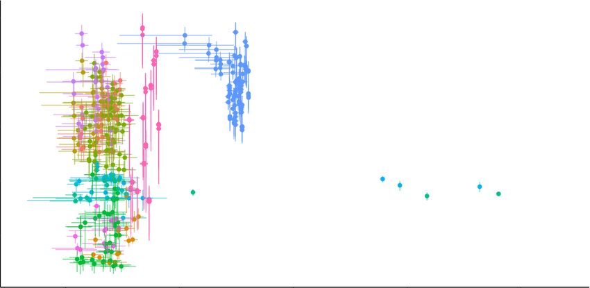
artificial neural networks, linear regression, extra trees       installed in each house, which monitor electricity usage
regression and support vector regression, which are al-          at short intervals, such as every 15 or 30 minutes. All
gorithms used in the literature [1, 12, 13].                     of the papers reviews in this subsection focus on offline
   We show that the forecasting algorithm has a non-             learning, as opposed to online learning like in this work.
negligible impact on carbon emissions and use of coal,           Additionally, we look at the long-term impact of poor
onshore, photovoltaics (PV), reciprocal gas engines and          predictions on the electricity market.
CCGT. Specifically, the amount of coal, PV, and recip-              Fard et al. propose a new hybrid forecasting method
rocal gas used from 2018 to 2035 was proportional to             based on the wavelet transform, autoregressive inte-
the median absolute error, while wind is inversely pro-          grated moving average (ARIMA) and artificial neu-
portional to the median absolute error.                          ral network (ANN) [20]. The ARIMA method is uti-
   Total investments in coal, offshore and photovoltaics         lized to capture the linear component of the time se-
are proportional to the median absolute error, while in-         ries, with the residuals containing the non-linear com-
vestments in CCGT, onshore and reciprocal gas engines            ponents. The non-linear parts are decomposed using
are inversely proportional.                                      the discrete wavelet transform which finds the sub-
   In this work, we make the following contributions:            frequencies. These residuals are then used to train an
                                                                 ANN to predict the future residuals. The ARIMA and
 1. The evaluation of different online and offline learn-        ANNs outputs are then summed. Their results show that
    ing algorithms to forecast the electricity demand            this technique can improve forecasting results.
    profile 24 hours ahead. This work extends previ-                Humeau et al. compare MLPs, SVRs and linear re-
    ous work by utilizing a vast array of different on-          gression at forecasting smart meter data [21]. They ag-
    line and offline techniques.                                 gregate different households and observe which algo-
 2. Evaluation of poor predictive ability on the long-           rithms work the best. They find that linear regression
    term electricity market in the UK through the per-           outperforms both MLP and SVR when forecasting indi-
    turbation of demand in the novel ElecSim simula-             vidual households. However, after aggregating over 32
    tion. There remains a gap in the literature of the           households, SVR outperforms linear regression.
    long-term impact of poor electricity demand pre-                Quilumba et al. also apply machine learning tech-
    dictions on the electricity market.                          niques to individual households’ electricity consump-
   In Section 2, we review the literature. We introduce          tion by aggregation [20]. To achieve this aggregation,
the dynamics of the ElecSim simulation as well as the            they use k-means clustering to aggregate the households
methods used in Section 3. We demonstrate the method-            to improve their forecasting ability. The authors also use
ology undertaken in Section 4. In Section 5 we demon-            a neural network based algorithm for forecasting, and
strate our results, followed by a discussion in Section 6.       show that the number of optimum clusters for forecast-
We conclude our work in Section 7.                               ing is dependent on the data, with three clusters optimal
                                                                 for a particular dataset, and four for another.
                                                                    In our previous work, we evaluate the performance
2. Literature Review                                             of ANNs, random forests, support vector regression and
                                                                 long short-term memory neural networks [2]. We uti-
   Multiple papers have looked at demand-side fore-
                                                                 lize smart meter data, and cluster by household using
casting [10]. These include both artificial intelligence
                                                                 the k-means clustering algorithm to aggregate groups of
[14, 15, 16] and statistical techniques [6, 17]. In addi-
                                                                 demand. Through this clustering we are able to reduce
tion to this, our research models the impact of the per-
                                                                 the error, with the random forest performing the best.
formance of different algorithms on investments made,
electricity sources dispatched and carbon emissions
over a 17 year period. To model this, we use the long-           2.2. Online learning
term electricity market agent-based model, ElecSim [9].             There have been several studies in diverse applica-
                                                                 tions on the use of online machine learning to predict
2.1. Offline learning                                            time-series data, however, to the best of our knowledge
   Multiple electricity demand forecasting studies have          there are limited examples where this is applied to elec-
been undertaken for offline learning [13, 18, 19]. Stud-         tricity markets. In our work, we trial a range of algo-
ies have been undertaken using both smart meter data,            rithms to our problem. Due to time constraints, we do
as well as with aggregated demand, similar to the work           not trial the additional techniques discussed in this liter-
in this paper. Smart meters are a type of energy meter           ature review within our paper.
                                                             3
The impact of online machine-learning methods on long-term investment decisions and generator utilization in electricity markets
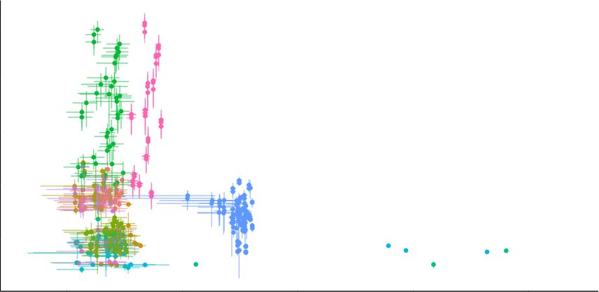
Johansson et al. apply online machine learning al-             posed to a local market.
gorithms for heat demand forecasting [22]. They find
that their demand predictions display robust behaviour
within acceptable error margins. They find that artificial        3. Material
neural networks (ANNs) provide the best forecasting
ability of the standard algorithms and can handle data               Examples of online learning algorithms are Passive
outside of the training set. Johansson et al., however, do        Aggressive (PA) Regressor [28], Linear Regression,
not look at the long-term effects of different algorithms,        Box-Cox Regressor [29], K-Neighbors Regressor [30]
which is a central part to this work.                             and Multilayer perceptron regressor [31]. For our work,
   Baram et al. combine an ensemble of active learners            we trial the stated algorithms, in addition to a host of
by developing an active-learning master algorithm [23].           offline learning techniques. The offline techniques tri-
To achieve this, they propose a simple maximum en-                alled were Lasso regression [32], Ridge regression [33],
tropy criterion that provides effective estimates in real-        Elastic Net [34], Least Angle Regression [35], Extra
istic settings. Their active-learning master algorithm is         Trees Regressor [35], Random Forest Regressor [36],
shown to, in some cases, outperform the best algorithm            AdaBoost Regressor [37], Gradient Boosting Regressor
in the ensemble on a range of classification problems.            [38] and Support vector regression [39]. We chose the
   Schmitt et al also extends on existing algorithms              boosting and random forest techniques due to previous
through an extension of the FLORA algorithm in [24,               successes of these algorithms when applied to electric-
25]. The FLORA algorithm generates a rule-based al-               ity demand forecasting [11]. We trialled the additional
gorithm, which has the ability to make binary decisions.          algorithms due to availability of these algorithms using
Their FLORA-MC enhances the FLORA algorithm for                   the packages scikit-learn and Creme [40, 41].
multi-classification and numerical input values. They             Linear regression. Linear regression is a linear ap-
use this algorithm for an ambient computing applica-              proach to modelling the relationship between a depen-
tion. Ambient computing is where computing and com-               dent variable and one or more independent variables.
munication merges into everyday life. They find that              Linear regressions can be used for both online and of-
their algorithm outperforms traditional offline learners.         fline learning. In this work, we used them for both on-
Our work focuses on electricity demand, however.                  line and offline learning. Linear regression algorithms
   Similarly to us, Pindoriya et al. trial several differ-        are often fitted using the least squares approach. The
ent machine learning methods such as adaptive wavelet             least squares approach minimizes the sum of the squares
neural network (AWNN) for predicting electricity price            of the residuals.
forecasting [26]. They find that AWNN has good pre-                  Other methods for fitting linear regressions are by
diction properties when compared to other forecasting             minimizing a penalized version of the least squares cost
techniques such as wavelet-ARIMA, multilayer percep-              function, such as in ridge and lasso regression [32, 33].
tron (MLP) and radial basis function (RBF) neural net-            Ridge regression is a useful approach for mitigating the
works. We, however, focus on electricity demand.                  problem of multicollinearity in linear regression. Mul-
   Goncalves Da Silva et al. show the effect of predic-           ticollinearity is where one predictor variable can be lin-
tion accuracy on local electricity markets [27]. They             early predicted from the others with a high degree of
compare forecasting of groups of consumers. They trial            accuracy. This phenomenon often occurs in algorithms
the use of the Seasonal-Naı̈ve and Holt-Winters algo-             with a large number of parameters.
rithms and look at the effect that the errors have on trad-          In ridge regression, the OLS loss function is aug-
ing in an intra-day electricity market of consumers and           mented so that we not only minimize the sum of squared
prosumers. They found that with a photovoltaic pene-              residuals but also penalized the size of parameter esti-
tration of 50%, over 10% of the total generation capac-           mates, in order to shrink them towards zero:
ity was uncapitalized and roughly 10, 25 and 28% of the                           n
                                                                                  X                    m
                                                                                                       X
total traded volume were unnecessary buys, demand im-             Lridge (β̂) =     (yi − xi0 β̂)2 + λ   βˆ2j = ||y − X β̂||2 + λ||β̂||2 .
balances and unnecessary sells respectively. This repre-                          i=1                   j=1
sents energy that the participant has no control. Uncap-                                                                (1)
italized generation capacity is where a participant could         Where λ is the regularization penalty which can be cho-
have produced energy, however, it was not sold on the             sen through cross-validation, or the value that mini-
market. Additionally, due to forecast errors, the partici-        mizes the cross-validated sum of squared residuals, for
pant might have sold less than it should have. Our work,          instance. n is the number of observations of the response
however, focuses on a national electricity market, as op-         variable, Y, with a linear combination of m predictor
                                                              4
variables, X, and we solve for β̂, where β̂ are the OLS                           power of the model [37]. By doing this, the dimension-
parameter estimates. Where yi is the outcome and xi are                           ality of the algorithm is reduced and can improve com-
the covariates, both for the ith case.                                            pute time. This can be used in conjunction with multiple
   Lasso is a linear regression technique which performs                          different algorithms. In our paper, we utilized the deci-
both variable selection and regularization. It is a type                          sion tree based algorithm with AdaBoost.
of regression that uses shrinkage. Shrinkage is where                                Random Forests are an ensemble learning method for
data values are shrunk towards a central point, such as                           classification and regression [36]. Ensemble learning
the mean. The lasso algorithm encourages models with                              methods use multiple learning algorithms to obtain bet-
fewer parameters and automates variable selection.                                ter predictive performance. They work by constructing
   Under Lasso the loss is defined as:                                            multiple decision trees and output the predicted value
                            n
                            X                          m
                                                       X                          that is the mode of the predictions of the trees.
            Llasso (β̂) =         (yi − xi0 β̂)2 + λ         |β̂ j |.   (2)           To ensure that the individual decision trees within a
                            i=1                        j=1                        Random Forest are not correlated, bagging is used to
   The only difference between lasso and ridge regres-                            sample from the data. Bagging is the process of ran-
sion is the penalty term.                                                         domly sampling with replacement of the training set and
   Elastic net is a regularization regression that linearly                       fitting the trees. This has the benefit of reducing the
combines the penalties of the lasso and ridge methods.                            variance of the algorithm without increasing the bias.
Specifically, Elastic Net aims to minimize the following                             Random Forests differ in one way from this bagging
loss function:                                                                    procedure. Namely, using a modified tree learning al-
                                                                                gorithm that selects, at each candidate split in the learn-
              i=1 (yi − xi β̂)
             Pn                                m           m
                         0 2
                                     1 − α X          X                    ing process, a random subset of the features, known as
Lenet (β̂) =                   +λ             β̂ j + α
                                                   2
                                                              |βˆj | ,
                    2n                     2 j=1          j=1
                                                                                  feature bagging. Feature bagging is undertaken due to
                                                                (3)               the fact that some predictors with a high predictive abil-
where α is the mixing parameter between ridge (α = 0)                             ity may be selected many times by the individual trees,
and lasso (α = 1). The parameters λ and α can be tuned.                           leading to a highly correlated Random Forest.
   Least Angle Regression (LARS) provides means of                                   ExtraTrees adds one further step of randomization
producing an estimate of which variables to include in a                          [35]. ExtraTrees stands for extremely randomized trees.
linear regression, as well as their coefficients.                                 There are two main differences between ExtraTrees and
Decision tree-based algorithms. The decision tree is an                           Random Forests. Namely, each tree is trained using the
algorithm which goes from observations to output using                            whole learning sample (And not a bootstrap sample),
simple decision rules inferred from data features [42].                           and the top-down splitting in the tree learner is random-
To build a regression tree, recursive binary splitting is                         ized. That is, instead of computing an optimal cut-point
used on the training data. Recursive binary splitting is a                        for each feature, a random cut-point is selected from a
greedy top-down algorithm used to minimize the resid-                             uniform distribution. The split that yields the highest
ual sum of squares. The RSS, in the case of a partitioned                         score is then chosen to split the node.
feature space with M partitions, is given by:                                     Gradient Boosting. Gradient boosting is also an ensem-
                              M X
                              X                                                   ble algorithm [38]. Gradient boosting optimizes a cost-
                   RS S =                (y − ŷRm )2 .                 (4)       function over function space by iteratively choosing a
                              m=1 i∈Rm                                            function that points in the negative gradient descent di-
                                                                                  rection, known as a gradient descent method.
Where y is the value to be predicted and ŷ is the pre-
dicted value for partition Rm .                                                   Support vector regression (SVR). SVR is an algorithm
   Beginning at the top of the tree, a split is made into                         which finds a hyperplane and decision boundary to map
two branches. This split is carried out multiple times                            an input domain to an output [39]. The hyperplane is
and the split is chosen that minimizes the current RSS.                           chosen by minimizing the error within a tolerance.
To obtain the best sequence of subtrees cost complexity,                            Suppose                we           have         the   training   set:
pruning is used as a function of α. α is a tuning param-                          (x1 , y1 ), . . . , (xi , yi ), . . . , (xn , yn ), where xi is the in-
eter that balances the depth of the tree and the fit to the                       put, and yi is the output value of xi . Support Vector
training data.                                                                    Regression solves an optimization problem [13, 43],
   The AdaBoost training process selects only the fea-                            under given parameters C > 0 and ε > 0, the form of
tures of an algorithm known to improve the predictive                             support vector regression is [44]:
                                                                              5
Inputs        Hidden Units           Outputs
                                                                                    the training set, and m observations in the test set,
             x1                   w11         m1                                    yN+1 , yN+2 , . . . , yN+m , and we are required to predict m
                                                       T1                           periods ahead [47]. The training patterns are as follows:
             x2

                                            ….
                                                                      y
                                                                                               y p+m = fW (y p , y p−1 , . . . , y1 )              (7)
                         ….

                                                       Tk

             xn                  wnk         mk
                                                                                            y p+m+1 = fW (y p+1 , y p , . . . , y2 )               (8)
                                                                                                   ..
       Figure 1: A three-layer feed forward neural network.
                                                                                                    .
                                                                                                 yN = fW (yN−m , yN−m−1 , . . . , yN−m−p+1 )       (9)

                                                   n                                where fW (·) represents the MLP network and W are
                          1       X
                   min ∗ ωT ω + C     (ξi + ξi∗ )                         (5)       the weights. For brevity we omit W. The training
                  ω,b,ξ,ξ 2
                                  i=1                                               patterns use previous time-series points, for example,
subject to                                                                          y p , y p−1 , . . . , y1 as the time series is univariate. That is,
                                                                                    we only have the time series in which we can draw in-
                  yi − (ωT φ(xi ) + b) ≤ ε + ξi∗ ,                                  ferences from. In addition, these time series points are
                   (ωT φ(xi ) + b) − yi ≤ ε + ξi ,                        (6)       correlated, and therefore provide information that can
                                ξi , ξi∗   ≥ 0, i = 1, . . . , n                    be used to predict the next time point.
                                                                                        The m testing patterns are
xi is mapped to a higher dimensional space using the
function φ. The ε-insensitive tube (ωT φ(xi ) + b) − yi ≤
ε is a range in which errors are permitted, where b is                                    yN+1 = fW (yN+1−m , yN−m , . . . , yN−m−p+2 )          (10)
the intercept of a linear function. ξi and ξi∗ are slack                                  yN+2 = fW (yN+2−m , yN−m+1 , . . . , yN−m−p+3 )        (11)
variables which allow errors for data points which fall
                                                                                              ..
outside of ε. This enables the optimization to take into                                       .
account the fact that data does not always fall within the
                                                                                         yN+m = fW (yN , yN−1 , . . . , yN−p+1 ).                (12)
ε range [45].
   The constant C > 0 determines the trade-off between                                  The training objective is to minimize the overall pre-
the flatness of the support vector function. ω is the al-                           dictive mean sum of squared estimate of errors (SSE)
gorithm fit by the SVR. The parameters which control                                by adjusting the connection weights. For this network
regression quality are the cost of error C, the width of                                                                 PN
                                                                                    structure the SSE can be written as i=p+m   (yi − ŷi ) where
the tube ε, and the mapping function φ [43, 13].                                    ŷi is the prediction from the network. The number of
K-Neighbors Regressor. K-Neighbors regression is a                                  input nodes corresponds to the number of lagged obser-
non-parametric method [30]. The input consists of a                                 vations. Having too few or too many input nodes can
new data point, and the algorithm finds the k closest                               affect the predictive ability [47].
training examples in the feature space. The output is                                   It is also possible to vary the the number of input
the mean value of the k nearest neighbours.                                         units. Typically, various different configurations of units
Multilayer perceptron. A neural network can be used in                              are trialled, with the best configuration being used in
offline and online cases. Here, we used them for both.                              production. The weights W in fW are trained using
   Artificial Neural Networks is an algorithm which can                             a process called backpropagation, which uses labelled
model non-linear relationships between input and out-                               data and gradient descent to optimize the weights.
put data [46]. A popular neural network is a feed-
forward multilayer perceptron. Fig. 1 shows a three-
                                                                                    3.1. Online Algorithms
layer feed-forward neural network with a single output
unit, k hidden units, n input units. wi j is the connection                         Box-Cox regressor. In this subsection, we discuss the
weight from the ith input unit to the jth hidden unit, and                          Box-Cox regressor. Ordinary least square is a method
T j is the connecting weight from the jth hidden unit to                            for estimating the unknown parameters in a linear re-
the output unit [47]. These weights transform the input                             gression algorithm. It estimates these unknown param-
variables in the first layer to the output variable in the                          eters by the principle of least squares. Specifically, it
final layer using the training data.                                                minimizes the sum of the squares of the differences be-
   For a univariate time series forecasting problem,                                tween the observed variables and those predicted by the
suppose we have N observations y1 , y2 , . . . , yN in                              linear function.
                                                                                6
The ordinary least squares regression assumes a nor-
mal distribution of residuals. However, when this is not
the case, the Box-Cox Regression may be useful [29].
It transforms the dependent variable using the Box-Cox
Transformation function and employs maximum likeli-
hood estimation to determine the optimal level of the
power parameter lambda.
Passive-Aggressive regressor. The goal of the Passive-
Aggressive (PA) algorithm is to change itself as little as
possible to correct for any mistakes and low-confidence
predictions it encounters [28]. Specifically, with each
                                                                             Figure 2: System overview of ElecSim [8].
example PA solves the following optimisation [48]:

               1
  wt+1 ← argmin ||wt − w||2 s.t. yi (w · xt ) ≥ 1.     (13)       by power plants through the use of a spot market. Gen-
               2                                                  erator companies invest in power plants based upon in-
Where xt is the input data and yi the output data, and            formation provided by the data sources and expectation
wt are the weights for the PA algorithm and w is the              of the data provided by the configuration file.
weight to be optimised. Updates occur when the inner                 ElecSim uses a configuration file which details the
product does not exceed a fixed confidence margin - i.e.,         scenario which can be set by the user. This includes
yi (w · xt ) ≥ 1. The closed-form update for all examples         electricity demand, carbon price and fuel prices. The
is as follows:                                                    data sources parametrize the ElecSim simulation to a
                                                                  particular country, including information such as wind
                     wt+1 ← wt + αt yt xt            (14)
                                                                  capacity and power plants in operation. A spot market
where                                                             then matches electricity demand with supply.
                        (                        )
                            1 − yt (wt · xt )                        The market runs a merit-order dispatch model, and
             αt = max                         , 0  .   (15)       bids are made by the power plant’s short-run marginal
                                ||xt ||2
                                                                  cost (SRMC). A merit-order dispatch model is one
at is derived from a derivation process which uses the            which dispatches the cheapest electricity generators
Lagrange multiplier [28].                                         first. SRMC is the cost it takes to dispatch a single MWh
                                                                  of electricity and does not include capital costs. Invest-
3.2. Long-term Energy Market Model                                ment in power plants is based upon a net present value
                                                                  (NPV) calculation. NPV is the difference between the
   In order to test the impact of the different residual          present value of cash inflows and the present value of
distributions, we used the ElecSim simulation [8, 9].             cash outflows over a period of time. This is shown in
ElecSim is an agent-based model which mimics the be-              Equation 16, where t is the year of the cash flow, i is the
haviour of decentralized electricity markets. In this pa-         discount rate, N is the total number of years, or lifetime
per, we parametrized the model with data of the United            of power plant, and Rt is the net cash flow of the year t:
Kingdom in 2018. This enabled us to create a digital
                                                                                                  N
twin of the UK electricity market and project forward.                                            X        Rt
The data used for this parametrization included power                             NPV(t, N) =                    .       (16)
                                                                                                  t=0
                                                                                                        (1 + i)t
plants in operation in 2018 and the funds available to
the GenCos [49, 50].                                              Each of the Generator Companies (GenCos) estimate
   ElecSim is made up of six components: 1) power                 the yearly income for each prospective power plant by
plant data; 2) scenario data; 3) the time-steps of the al-        running a merit-order dispatch electricity market simu-
gorithm; 4) the power exchange; 5) the investment al-             lation ten years into the future. However, it is true that
gorithm and 6) the GenCos as agents. ElecSim uses                 the expected cost of electricity ten years into the future
a subset of representative days of electricity demand,            is particularly challenging to predict. We, therefore,
solar irradiance and wind speed to approximate a full             use a reference scenario projected by the UK Govern-
year. Representative days are a subset of days which,             ment Department for Business and Industrial Strategy
when scaled up, represent an entire year [9]. We show             (BEIS), and use the predicted costs of electricity cali-
how these components interact in Figure 2 [8]. Namely,            brated by Kell et al [9, 51]. The agents predict the future
electricity demand is matched with the supply provided            carbon price by using a linear regression algorithm.
                                                              7
More concretely, the GenCos make investments by                 sons. Finally, to predict a full 24-hours ahead, we used
comparing the expected profitability of each of the                24 different algorithms, 1 for each hour of the day.
power plants over their respective lifetime. They invest              The data is standardized and normalized using min-
in the power plant which they deem to be the most prof-            max scaling between -1 and 1 before training and pre-
itable. A major uncertainty in power plant investment is           dicting with the algorithm. This is due to the fact that
the price of electricity whilst the power plant is in oper-        the inputs such as day of the week, hour of day are sig-
ation. This is often a 25 year period. This is where the           nificantly smaller than that of demand. Therefore, the
predicted costs of electricity calibrated in [9] is used.          demand will influence the result more due to its larger
                                                                   value. However, this does not necessarily mean that de-
                                                                   mand has greater predictive power.
4. Methods                                                         Algorithm Tuning. To find the optimum hyperparam-
                                                                   eters, cross-validation is used. As this time-series data
Data Preparation. Similarly to our previous work in                were correlated in the time-domain, we took the first six
[2], we selected a number of calendar attributes and de-           years of data (2011-2017) for training and tested on the
mand data from the GB National Grid Status dataset                 remaining year of data (2017-2018).
provided by the electricity market settlement company                 Each machine learning algorithm has a different set
Elexon, and the University of Sheffield [52]. This                 of parameters to tune. To tune the parameters in this
dataset contained data between the years 2011-2018 for             paper, we used a grid search method. Grid search is a
the United Kingdom. The calendar attributes used as                brute force approach that trials each combination of pa-
predictors to the algorithms were hour, month, day of              rameters at our choosing; however, for our search space
the week, day of the month and year. These attributes              was small enough to make other approaches not worth
allow us to account for the periodicity of the data within         the additional effort.
each day, month and year.                                             Tables 1 and 2 display each of the algorithms and re-
   It is also the case that electricity demand on a public         spective parameters that were used in the grid search.
holiday which falls on a weekday is dissimilar to load             Table 1 shows the offline machine learning methods,
behaviours of ordinary weekdays [14]. We marked each               whereas Table 2 displays the online machine learning
holiday day to allow the algorithm to account for this.            methods. Each of the parameters within the columns
   As demand data is highly correlated with historical             “Values” are trialled with every other parameter.
demand, we lagged the input demand data. In this con-                 Whilst there is room to increase the total number of
text, the lagged data is where we provide data of previ-           parameters, due to the exponential nature of grid-search,
ous time steps at the input. For example, for predicting           we chose a smaller subset of hyperparameters, and a
t + 1, we use n inputs: t, t − 1, t − 2, . . . , t − n. This       larger number of regressor types. Specifically, with neu-
enabled us to take into account correlations on previous           ral networks, there is a possibility to extend the num-
days, weeks and the previous month. Specifically, we               ber of layers as well as the number of neurons, to use a
used the previous 28 hours before the time step to be              technique called deep learning. Deep learning is a class
predicted for the previous 1st, 2nd, 7th and 30th day.             of neural networks that use multiple layers to extract
We chose this as we believe that the previous two days             higher levels of features from the input. For this paper,
were the most relevant to the day to be predicted, as well         however, we decided to trial a large number of different
as the weekday of the previous week and the previous               algorithms, instead of a large number of different con-
month. We chose the previous 28 hours to account for               figurations for neural networks.
a full day, plus an additional 4 hours to account for the          Implementation methodology. The implementation
previous day’s correlation with the day to be predicted.           slightly differs between online and offline learning. In
We could have increased the number of days provided to             offline learning, batch processing occurs. That is, all
the algorithm. However, due to time and computational              the data from 2011 to 2017 is used to train the algo-
constraints, we used our previously described intuition            rithm. Once each of the algorithms had been trained,
for lagged data selection.                                         the algorithms are used to predict the electricity de-
   In addition to this, we marked each of the days with            mand from 2017 to 2018. For hyper-parameter tun-
their respective seven seasons. These seasons were de-             ing cross-validation is used. Specifically, the training
fined by the National Grid Short Term Operating Re-                data is randomly split ten times to select the best hyper-
serve (STOR) Market Information Report [53]. These                 parameters. This allowed for an unbiased assessment of
differ from the traditional four seasons by splitting au-          the data.
tumn into two further seasons, and winter into three sea-             For online learning a similar process is undertaken.
                                                               8
That is, the algorithms are trained in a batched approach
                                                                                                                                                                                                                                                                                              using data from 2011 to 2017. Between the year 2017
                                                                                                                                                                                                                                                                                              and 2018, the next time-step is predicted and the error
                                                                                                                                                                                                                                                                                              recorded between actual value and the predicted value.
                                                                                                                                                                                                                                                                                              Next, the algorithm is updated using the actual value,
                                                                                                                                                                                                                                                                                              and the next value predicted again.

                                                                                                                                                                                                                               K-Neighbours
                                                                                                                                                                                                                               Multilayer Perceptron
                                                                                                                                                                                                                               Support Vector
                                                                                                                                                                                                                               Gradient Boosting
                                                                                                                                                                                                                               Extra Trees, Random Forest, AdaBoost
                                                                                                                                                                                                                               Linear, Lasso, Elastic Net, Least-Angle
                                                                                                                                                                                                                                                                         Regressor Type
                                                                                                                                                                                                                                                                                              Prediction Residuals in ElecSim. Each of the algo-
                                                                                   Passive Aggressive

                                                                                                        Multilayer Perceptron
                                                                                                        Box-Cox
                                                                                                        Linear
                                                                                                                                Regressor Type

                                                                                                                                                                                                                                                                                              rithms trialled will have a degree of error. Prediction
                                                                                                                                                                                                                                                                                              residuals are the difference between the estimated and
                                                                                                                                                                                                                                                                                              actual values. We collect the prediction residuals to
                                                                                                                                                                                                                                                                                              form a distribution for each of the algorithms. We then
                                                                                                                                                                                                                                                                                              trial 80 different closed-form distributions to see which
                                                                                                                                                                                                                                                                                              of the distributions best fits the residuals from each of
                                                                                                                                                                                                                                                                                              the algorithms. These 80 distributions were chosen due
                                                                                   C

                                                                                                        Hidden layer sizes
                                                                                                        Power
                                                                                                        N/A
                                                                                                                                Parameters

                                                                                                                                                                                                                                                                                              to their implementation in scikit-learn [40].
                                                                                                                                                                                                                                                                                                  Once each of the prediction residual distributions are
                                                                                                                                                 Table 1: Hyperparameters for offline machine learning regression algorithms
Table 2: Hyperparameters for online machine learning regression algorithms

                                                                                                                                                                                                                                                                                              fit with a sensible closed-form distribution, we sample
                                                                                                                                                                                                                                                                                              from this new distribution and perturb the demand for
                                                                                                                                                                                                                               # Neighbours
                                                                                                                                                                                                                               Activation function
                                                                                                                                                                                                                               Kernel
                                                                                                                                                                                                                               # Estimators
                                                                                                                                                                                                                               # Estimators
                                                                                                                                                                                                                               N/A
                                                                                                                                                                                                                                                                         Parameters

                                                                                                                                                                                                                                                                                              the electricity market at each time step within ElecSim.
                                                                                                                                                                                                                                                                                                  By perturbing the market by the residuals, we can ob-
                                                                                   [0.1, 1, 2]
                                                                                   (50), (10, 50)]
                                                                                   [(10, 50, 100), (10), (20),
                                                                                   [0.1, 0.05, 0.01]
                                                                                   N/A
                                                                                                                                Values

                                                                                                                                                                                                                                                                                              serve what the effects are of incorrect predictions of de-
                                                                                                                                                                                                                                                                                              mand in an electricity market using ElecSim.
                                                                                                                                                                                                                                                                                                  ElecSim has previously been validated in [9]. In this
                                                                                                                                                                                                                                                                                              work, we validated our algorithm between the years
                                                                                                                                                                                                                               [5, 20, 50]
                                                                                                                                                                                                                               [tanh, relu]
                                                                                                                                                                                                                               [linear, rbf]
                                                                                                                                                                                                                               [16, 32]
                                                                                                                                                                                                                               [16, 32]
                                                                                                                                                                                                                               N/A
                                                                                                                                                                                                                                                                         Values

                                                                                                                                                                                                                                                                                              2013 and 2018, and recorded the difference between ob-
                                                                                                                                                                                                                                                                                              served electricity mix to predicted electricity mix. We
                                                                                                                                                                                                                                                                                              found that we were able to predict each different elec-
                                                                                                                                                                                                                                                                                              tricity source better than the naive approach. The naive
                                                                                   Fit intercept?

                                                                                                                                Parameters

                                                                                                                                                                                                                                     hidden layer sizes
                                                                                                                                                                                                                                     C
                                                                                                                                                                                                                                     learning rate

                                                                                                                                                                                                                                                                         Parameters

                                                                                                                                                                                                                                                                                              approach, in this case, was predicting the electricity mix
                                                                                                                                                                                                                                                                                              at the last known point in 2013. However, we were able
                                                                                                                                                                                                                                                                                              to better predict coal, solar and wind by achieving a
                                                                                                                                                                                                                                                                                              mean absolute scaled error (MASE) of ∼0.4 for these.
                                                                                   [True, False]

                                                                                                                                Values

                                                                                                                                                                                                                                                                                              CCGT and nuclear on the other hand had slightly worse
                                                                                                                                                                                                                                                                                              results, achieving a MASE of ∼0.7.
                                                                                                                                                                                                                                     [1, 50]
                                                                                                                                                                                                                                     [1, 10]
                                                                                                                                                                                                                                     [0.8, 1.0]

                                                                                                                                                                                                                                                                         Values

                                                                                                                                                                                                                                                                                              5. Results
                                                                                   Max iterations

                                                                                                                                Parameters

                                                                                                                                                                                                                                     Alpha
                                                                                                                                                                                                                                     Gamma

                                                                                                                                                                                                                                                                         Parameters

                                                                                                                                                                                                                                                                                                 In this Section, we detail the accuracy of the algo-
                                                                                                                                                                                                                                                                                              rithms to predict 24 hours ahead for the day-ahead mar-
                                                                                                                                                                                                                                                                                              ket. In addition to this, we display the impact of the er-
                                                                                                                                                                                                                                                                                              rors on electricity generation investment and electricity
                                                                                                                                                                                                                                     [0.00005, 0.0005]
                                                                                                                                                                                                                                     [0.001, 0.0001]

                                                                                                                                                                                                                                                                         Values
                                                                             1000]
                                                                             [1, 10, 100,

                                                                                                                                Values

                                                                                                                                                                                                                                                                                              mix from the years 2018 to 2035 using the agent-based
                                                                                                                                                                                                                                                                                              model ElecSim.

                                                                                                                                                                                                                                                                                              5.1. Offline Machine Learning
                                                                                                                                                                                                                                                                                                 In this work, the training data was from 2011 to 2017,
                                                                                                                                                                                                                                                                                              and the testing data was from 2017 to 2018.
                                                                                                                                                                                                                                                                                                 Figure 3 displays the mean absolute error of each
                                                                                                                                                                                                                                                                                              of the offline statistical and machine learning algo-
                                                                                                                                                                                                                                                                                              rithms on a log scale. It can be seen that the differ-
                                                                                                                                                                                                                                                                                              ent algorithms have varying degrees of success. The
                                                                                                                                                                                                                                                                                          9
least accurate algorithms were linear regression, mul-

                                                                                Frequency of occurence
tilayer perceptron (MLP) and the Least Angle Regres-
                                                                                                         0.00015
sion (LARS), each with mean absolute errors over
10,000MWh. This error would be prohibitively high
in practice; the max tendered national grid reserve is                                                   0.00010
6,000MWh, while the average tendered national grid re-
serve is 2,000MWh [53].                                                                                  0.00005
   A number of algorithms perform well, with a low
mean absolute error. These include the Lasso, gradient
                                                                                                         0.00000
Boosting Regressor and K-neighbours regressor. The                                                                 −10000 −5000            0      5000         10000
best algorithm, similar to [2], was the decision tree-                                                                                  Residuals
based algorithm, Extra Trees Regressor, with a mean                                                         5% Percentile
absolute error of 1, 604MWh. This level is well within                                                      95% Percentile
the average national grid reserve of 2,000MWh.                                                              0
                                                                                                            Ma Tendered National Grid Reserve
   Table 3 displays different metrics for measuring the
                                                                                                            Average Available Tendered National Grid Reserve
accuracy of the offline machine learning techniques.
These include Mean Squared Error (MSE), Root Mean
                                                                                Figure 4: Best offline machine learning algorithm (Extra Trees Re-
Squared Error (RMSE), Mean Absolute Error (MAE)                                 gressor) distribution.
and the Mean R-Squared. The results largely compli-
ment each other. With high error values in one metric
correlating to high error metrics in others for each of the                     type for each algorithm. The error bars indicate the re-
estimators.                                                                     sults of multiple cross-validations.
                  Linear Regression
                                                                                   It can be seen from Figure 5 that the time to fit varies
                              Lasso                                             significantly between algorithms and parameter choices.
                              Ridge                                             The multilayer perceptron consistently takes a long time
                          ElasticNet
                                                                                to fit, when compared to the other algorithms and per-
Regressor Model

                               LARS
                        Extra Trees                                             forms relatively poorly in terms of MAE. There are
                     Random Forest
                          AdaBoost
                                                                                many algorithms, such as the random forest regressor,
                  Gradient Boosting                                             and extra trees regressors which perform well, however,
                                 SVR                                            take a long time to fit, especially when compared to the
                                 MLP
                       K-Neighbors
                                                                                K-Nearest neighbours.
                                       104                  105      106           For a small deterioration in MAE it is possible to de-
                                         Mean Absolute Error (Log)
                                                                                crease the time it takes to train the algorithm signifi-
Figure 3: Offline algorithms mean absolute error comparison, with               cantly. For example, by using the K-Nearest neighbours
95% confidence interval for 5 runs of each algorithm.                           or support vector regression (SVR).

   Figure 4 displays the distribution of the best offline                                           1e+03

machine result (Extra Trees Regressor). It can be seen
                                                                                Fit Time log10(S)

                                                                                                    1e+02
that the max tendered national grid reserve falls well
above the 5% and 95% percentiles. However, there are                                                1e+01

occasions where the errors are greater than the maxi-
                                                                                                    1e+00
mum tendered national grid reserve. In addition, the
majority of the time, the algorithm’s predictions fall                                              1e−01

within the average available tendered national grid re-
                                                                                                              1e+03        1e+04       1e+05           1e+06         1e+07
serve. Therefore, there is room for improvement, to                                                                       Mean Absolute Error log10(MAE)
ensure that blackouts do not occur and predictions fall                                                                     AdaBoost           ElasticNet      ExtraTrees
within the max tendered national grid reserve.                                                                Estimator
                                                                                                                            GradientBoosting   KNeighbors      LARS
                                                                                                                            Lasso              Linear          MLP
   Figures 5 and 6 display the time taken to train the al-                                                                  RandomForest       Ridge           SVR
gorithm and time taken to sample from the algorithm
versus the absolute error respectively for the offline al-                      Figure 5: Time taken to train the offline algorithms versus mean abso-
gorithms. Multiple fits are trialled for each parameter                         lute error. Error bars display standard deviation between points.

                                                                           10
Estimator                                           Mean Fit Time        Mean Score Time     Mean MSE                         Mean RMSE                    Mean MAE        Mean R-Squared
LinearRegression                                    57                   4.84                9444808.95                       3073.24                      2249.34         0.81
Lasso                                               787.97               3.13                9446957.22                       3073.59                      2249.55         0.81
Ridge                                               26.99                5.03                9444701.58                       3073.22                      2252.23         0.81
ElasticNet                                          54.49                6.13                31139231.96                      5580.25                      4628.64         0.36
llars                                               46.85                8                   10164815.45                      3188.23                      2333.31         0.79
ExtraTreesRegressor                                 9321.52              58.06               5562579.53                       2358.51                      1605            0.89
RandomForestRegressor                               16567.46             13.99               5882618.89                       2425.41                      1646.29         0.88
AdaBoostRegressor                                   8897.55              26.9                18551963.36                      4307.2                       3544.49         0.62
GradientBoostingRegressor                           6417.62              8.16                6744402.87                       2597                         1833.62         0.86
SVR                                                 19170.82             5221.66             51217167.5                       7156.62                      5926.75         -0.05
KNeighborsRegressor                                 118.89               15215.87            10107201.23                      3179.18                      2246.6          0.79

                                                               Table 3: Different metrics for offline machine learning results.

   The scoring time, displayed in Figure 6, also displays                                                              (PA) C = 0.1, fit intercept = false

a large variation between algorithm types. For instance,                                                                    (PA) C = 0.1, fit intercept = true

the MLP regressor takes a shorter time to sample predic-                                                                     (PA) C = 2, fit intercept = false

                                                                                                          Regressor Model
                                                                                                                              (PA) C = 2, fit intercept = true
tions when compared to the K-Neighbors algorithm and
                                                                                                                             MLP (all parameter variations)
support vector regression. It is possible to have a clus-                                                                             (Box Cox) power = 0.1
ter of algorithms with low sample times and low mean                                                                                       Linear Regression
absolute errors. However, often a trade-off is required,                                                                           Extra Trees (Best offline)
with a fast prediction time requiring a longer training                                                                                                      0   1000 2000 3000 4000 5000 6000
                                                                                                                                                                       Mean Absolute Error
time and vice-versa. Practitioners, therefore, must de-
cide which aspect is most important for them for their                                            Figure 7: Comparison of mean absolute errors (MAE) for different
use case: speed of training or of prediction.                                                     online regressor algorithms. MLP results for all parameters are shown
                                                                                                  in a single barchart due to the very similar MAEs for the differing
                                                                                                  hyperparameters.
                      1e+02
Score Time log10(S)

                      1e+01
                                                                                                  same results, we removed them. For the multilayer per-
                      1e+00                                                                       ceptron (MLP), we aggregated all hyperparameters, due
                      1e−01
                                                                                                  to the similar nature of the predictions.
                                                                                                     It can be seen that the best performing algorithm was
                      1e−02                                                                       the Box-Cox regressor, with an MAE of 1100. This is an
                                                                                                  improvement of over 30% on the best offline algorithm.
                              1e+03        1e+04       1e+05           1e+06         1e+07
                                          Mean Absolute Error log10(MAE)                          The other algorithms perform less well. However, it can
                                            AdaBoost           ElasticNet      ExtraTrees         be seen that the linear regression algorithm improves
                                            GradientBoosting   KNeighbors      LARS
                              Estimator                                                           significantly for the online case when compared to the
                                            Lasso              Linear          MLP
                                            RandomForest       Ridge           SVR                offline case. The passive aggressive (PA) algorithm im-
                                                                                                  prove significantly with the varying parameters, and the
Figure 6: Time taken to score the offline algorithm versus mean abso-                             MLP performs poorly in all cases.
lute error. Error bars display standard deviation between points.
                                                                                                     Table 4 displays the metrics for each of the online
                                                                                                  methods. This includes the mean MSE, mean RMSE
                                                                                                  and mean MAE. Again, the metrics largely correlate
5.2. Online Machine Learning                                                                      with each other. Meaning, that the favoured metric can
   To see if we can improve on the predictions, we uti-                                           be used when selecting an estimator.
lize an online machine learning approach. If we are suc-                                             Figure 8 displays the best online algorithm. We can
cessful, we should be able to reduce the national grid                                            see a significant improvement over the best online algo-
reserves, reducing cost and emissions.                                                            rithm distribution, shown in Figure 4. We remain within
   Figure 7 displays the comparison of mean absolute                                              the max tendered national grid reserve for 98.9% of the
errors for the different trialled online regressor algo-                                          time, and the average available tendered national grid
rithms. To produce this graph, we show various hyper-                                             reserve is close to the 5% and 95% percentiles. This
parameter trials. Where the hyperparameters had the                                               model, therefore would be highly recommended over
                                                                                             11
Estimator                             Mean Fit Time     Mean Score Time                              Mean MSE           Mean RMSE           Mean MAE
                               (PA) C = 0.1, fit intercept = false   173.52            24.63                                        103015609.55       9497.47             5888.4
                               (PA) C = 0.1, fit intercept = true    168.66            24.07                                        63201775.28        7430.63             4605.94
                               (PA) C = 2, fit intercept = false     165.23            23.75                                        7451087.49         2723.25             1927.33
                               (PA) C = 2, fit intercept = true      174.91            24.65                                        7223163.14         2681.2              1907.59
                               (MLP) (all parameter variations)      71.36             6.58                                         9612351.37         3076.77             2221.48
                               (Box Cox) power = 0.1                 38.61             4.88                                         2921934.52         1703.79             1214.95
                               Linear Regression                     38.61             4.85                                         5629651.14         2368.3              1785.02

                                                               Table 4: Different metrics for online machine learning results.

the best offline version to ensure demand is matched                                                                                0.00005

                                                                                                           Frequency of occurence
with supply.
                                                                                                                                    0.00004

                               0.00030                                                                                              0.00003
      Frequency of occurence

                               0.00025                                                                                              0.00002
                               0.00020                                                                                              0.00001
                               0.00015
                                                                                                                                    0.00000
                                                                                                                                                 −40000       −20000            0
                               0.00010
                                                                                                                                                              Residuals
                               0.00005                                                                                                5% Percentile
                                                                                                                                      95% Percentile
                               0.00000                                                                                                0
                                    −15000−10000 −5000   0    5000 10000
                                                    Residuals                                                                         Max Tendered National Grid Reserve
                                  5% Percentile                                                                                       Average Available Tendered National Grid Reserve
                                  95% Percentile
                                  0
                                                                                                  Figure 9: Online machine learning algorithm distribution. (Passive
                                  Max Tendered National Grid Reserve
                                  Average Available Tendered National Grid Reserve                Aggressive Regressor (C=0.1, fit intercept = true, maximum iterations
                                                                                                  = 1000, shuffle = false, tolerance = 0.001), chosen as it was the worst
                                                                                                  result for the passive aggressive algorithm.
 Figure 8: Best online algorithm (Box-Cox Regressor) distribution.
                                                                                                                       35000

   Figure 9 displays the residuals for a algorithm with
                                                                                                         Demand (MW)

poor predictive ability, the passive aggressive regressor.                                                             30000
                                                                                                                                                                                    Variable
It displays a large period of time of prediction errors                                                                                                                               Actuals
                                                                                                                                                                                      Box−Cox
                                                                                                                       25000
                                                                                                                                                                                      Extra Trees
at -20,000MWh, and often falls outside of the national
grid reserve. These results demonstrate the importance                                                                 20000

of trying a multitude of different algorithms and param-                                                                              0         50          100           150
eters to improve prediction accuracy.                                                                                                                Hour of Week

   Figure 10 displays a comparison between the actual                                             Figure 10: Best offline algorithm compared to the best online algo-
electricity consumption compared to the predictions. It                                           rithm over a one week period.
can be seen that the Box-Cox algorithm better predicts
the actual electricity demand in most cases when com-
pared to the best offline algorithm, the Extra Trees re-                                             Clear clusters can be seen between different types of
gressor. The Extra Trees regressor often overestimates                                            algorithms and parameter types. With the passive ag-
the demand, particularly during weekdays. Whilst the                                              gressive (PA) algorithm performing the slowest for both
Box-Cox regressor more closely matches the actual re-                                             training and testing. Different parameter combinations
sults. During the weekend (between the hours of 120                                               show different results in terms of mean absolute error.
and 168), the Extra Trees regressor performs better, par-                                            The best performing algorithm is the Box-Cox algo-
ticularly on the Saturday (between hours of 144 and                                               rithm, which is also the fastest to both train and test. The
168).                                                                                             linear regression, which performs worse in terms of pre-
   Figures 11 and 12 display the mean absolute error                                              dictive performance, is as quick to train and test as the
versus test and training time respectively. In these                                              Box-Cox algorithm. Additionally, the multilayer per-
graphs, a selection of algorithms and parameter com-                                              ceptron (MLP) is relatively quick to train and test when
binations are chosen.                                                                             compared to the PA algorithms. We, therefore, recom-
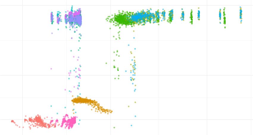
                                                                                            12
mend the Box-Cox algorithm as an optimal for training                                                                                                                                        5.3.1. Mean Contributed Energy Generation
and testing speed as well as accuracy.                                                                                                                                                          In this Section we display the mean electricity mix
   It is noted that when compared to the offline algo-                                                                                                                                       contributed by different electricity sources from 2018 to
rithms, the training time is a good indicator to the test-                                                                                                                                   2035.
ing time. In other words, algorithms that are fast to train                                                                                                                                     Figure 13 displays the mean power contributed be-
are also fast to test and vice-versa.                                                                                                                                                        tween 2018 and 2035 for each source vs. mean abso-
                      30
                                                                                                                                                                                             lute error of the various online regressor algorithms dis-
                                                                                                                                                                                             played in Figure 7. A positive correlation can be seen
                                                                                                                                                                                             with PV contributed and mean absolute error. This is
Score Time log10(S)

                                                                                                                                                                                             similar for coal and nuclear output. However, it can be
                                                                                                                                                                                             seen that offshore wind reduces with mean absolute er-
                      10
                                                                                                                                                                                             ror. Output for the reciprocal gas engine also increases
                                                                                                                                                                                             with mean absolute error.
                       5
                                                                                                                                                                                                The reciprocal gas engine was expected to increase
                                                                                                                                                                                             with times of high error. This is because, traditionally,
                                                      1000                                   3000                                         10000
                                                                               Mean Absolute Error log10(MAE)                                                                                reciprocal gas engines are peaker power plants. Peaker
                       (Box Cox) power = 0.1                                                      (PA) = (PA) C = 2, fit_intercept = false       (PA) C = 2, fit_intercept = true
                       (MLP) hidden_layer_sizes = 10
                       (PA) = (PA) C = 0.1, fit_intercept = false
                                                                                                  (PA) = (PA) C = 2, fit_intercept = true
                                                                                                  (PA) C = 0.1, fit_intercept = false
                                                                                                                                                 Linear Regression                           power plants provide power at times of peak demand,
                       (PA) = (PA) C = 0.1, fit_intercept = true                                  (PA) C = 2, fit_intercept = false
                                                                                                                                                                                             which cannot be covered by other plants due to them
Figure 11: Time taken to test the online algorithms versus mean abso-                                                                                                                        being at their maximum capacity level or out of service.
lute error.                                                                                                                                                                                  It may also be the case, that with higher proportions of
                                                                                                                                                                                             intermittent technologies, there is a larger need for these
                                                                                                                                                                                             peaker power plants to fill in for times where there is a
                                                                                                                                                                                             deficit in wind speed and solar irradiance.
                                                                                                                                                                                                It is hypothesized that coal and nuclear output in-
                           Training Time log10(S)

                                                    100
                                                                                                                                                                                             crease to cover the predicted increased demands of the
                                                                                                                                                                                             service. As these generation types are dispatchable,
                                                                                                                                                                                             meaning operators can choose when they generate elec-
                                                     50
                                                                                                                                                                                             tricity, they are more likely to be used in times of higher
                                                                                                                                                                                             predicted demand.
                                                     30
                                                             1000                                    3000                                    10000
                                                                                     Mean Absolute Error log10(MAE)
                                                                                                                                                                                             5.3.2. Total Energy Generation
                                                     (Box Cox) power = 0.1                            (PA) = (PA) C = 2, fit_intercept = false       (PA) C = 2, fit_intercept = true
                                                     (MLP) hidden_layer_sizes = 10                    (PA) = (PA) C = 2, fit_intercept = true        Linear Regression
Model                                                (PA) = (PA) C = 0.1, fit_intercept = false
                                                     (PA) = (PA) C = 0.1, fit_intercept = true
                                                                                                      (PA) C = 0.1, fit_intercept = false
                                                                                                      (PA) C = 2, fit_intercept = false
                                                                                                                                                                                                In this Section, we detail the difference in total tech-
                                                                                                                                                                                             nologies invested in over the time period between 2018
Figure 12: Time taken to train the online algorithms versus mean ab-                                                                                                                         to 2035, as predicted by ElecSim.
solute error.
                                                                                                                                                                                                CCGT, onshore, and reciprocal gas engines invest-
                                                                                                                                                                                             ment is less with an increase in MAE, as shown in Fig-
                                                                                                                                                                                             ure 14. While coal, offshore, nuclear and photovoltaics
5.3. Scenario Comparison                                                                                                                                                                     all exhibit increasing investments with MAE. Therefore,
   In this Section we explore the effect of these residuals                                                                                                                                  a smaller error leads to an increased usage of onshore
on investments made and the electricity generation mix.                                                                                                                                      wind, where lulls in wind supply are covered by CCGT
To generate these graphs, we perturbed the exogenous                                                                                                                                         and reciprocal gas engines.
demand in ElecSim by sampling from the best-fitting                                                                                                                                             It is hypothesized that coal and nuclear increase in
distributions for the respective residuals of each of the                                                                                                                                    investment due to their dispatchable nature. While on-
online methods. We did this for all of the online learning                                                                                                                                   shore, non-dispatchable by nature, become a less attrac-
algorithms displayed in Figure 7. We let the simulation                                                                                                                                      tive investment.
run for 17 years from 2018 to 2035.                                                                                                                                                             CCGT and reciprocal gas engines may have de-
   Running this simulation enabled us to see the effect                                                                                                                                      creased in capacity over this time, due to the increase
on carbon emissions on the electricity grid over a long                                                                                                                                      in coal. This could be because of the large consistent
time period. For instance, does underestimating elec-                                                                                                                                        errors in prediction accuracy that meant that reciprocal
tricity demand mean that peaker power plants, such as                                                                                                                                        gas engines were perceived to be less valuable.
reciprocal gas engines, are over utilized when other, less                                                                                                                                      Figure 15 shows an increase in relative mean car-
polluting power plants could be used?                                                                                                                                                        bon emitted with mean absolute error of the predic-
                                                                                                                                                                                        13
CCGT                                     Coal                                    Nuclear                       Offshore                                                                   Onshore                                PV                                Recip_gas
generated (MWh)

                           ●
                                                                   ●
                                                                   ●
                                                                                                   325000                         ●               ●

                                                                                                                                                  ●
                                                                                                                                                                                                                         ●
                                                                                                                                                                                                                                                            ●
                                                                                                                                                                                                                                                                              ●

                                                                                                                                                                                                                                                                                              1000
                  420000
                           ●
                           ●
                                                   ●

                                                                                                                                      26200                                                                          ●
                                                                                                                                                                                                                                                   725000
   Total mean

                                                           67000                       ●       ●
                                                                                                                                                  ●
                                                                                                                                                      ●
                                                                                                                                                                            32000                                                                                                                        ●
                                                                                                                                                                                                                                                                                                         ●
                                                                                                                                                                                                                                                                                                                  ●

                                                                                                   300000                                         ●                 ●
                                                                                                                                                                                                                                           ●

                                                                                                                                                                                                                                                                                              950
                                                                                                                                                                                                                                                                                                                      ●

                  410000                                   65000   ●

                                                                   ●
                                                                                       ●

                                                                                                                ●
                                                                                                                                      26100                             ●
                                                                                                                                                                        ●
                                                                                                                                                                                                                         ●                         700000                     ●

                                                                                                                                                                                                                                                                                                       ●
                                                                                                                                                                                                                                                                                                                  ●
                                                                                                                                                                                                                                                                                                                      ●

                                                                                                                                                                            30000
                           ●                       ●                                                                                              ●                 ●                                                                                       ●                                         ●
                                           ●                            ●
                                                                                                                                                                                                                                                            ●                         ●

                                                                                                   275000
                                                                   ●                           ●                                                                                                                         ●

                                                                                                                                      26000                                                                                                                                                   900
                                                                                                                                                                                                                                                                                                          ●

                  400000                                   63000                                                    ●
                                                                                                                                                                                                                         ●
                                                                                                                                                                                                                                                   675000   ●
                                                                                                                                                                                                                                                            ●
                                                                                                                                                                                                                                                                                                              ●

                                                                                                                                                                                                                                               ●
                                                                                                                                                                                                                                               ●
                                   ●                                                                            ●                                                                                                                          ●                                          ●

                                                                                                                                      25900
                                                                                                                ●

                  390000
                           ●

                                           ●               61000                                   250000      ●
                                                                                                                ●
                                                                                                                ●
                                                                                                                              ●   ●
                                                                                                                                                                            28000                                        ●
                                                                                                                                                                                                                             ●                     650000           ●

                                                                                                                                                                                                                                                                                              850
                           ●                                       ●
                                                                                                                      25800   ●
                                                                                                                                                  ●
                                                                                                                                                                                                                                625000                      ●                                             ●

                       3000 12000                              3000 12000                                  3000 12000      3000 12000                                                                                3000 12000       3000 12000                                                    3000 12000
                                                                                                                                      Mean Absolute Error

                                         Figure 13: Mean outputs of various technologies vs. mean absolute error from 2018 to 2035 in ElecSim.

                                       CCGT                                     Coal                                    Nuclear                       Offshore                                                                   Onshore                                PV                            Recip_gas
generated (MWh)

                  230000       ●                                                                                                  ●                                                                                  ●

                                                                                                                                                                                                                                                   360000       ●
                                                                                                                                                                                                                                                                                              420                 ●

                  220000                                                                               21000                                                                                                         ●
   Total mean

                                                                                                                                                                                                                                           ●

                                                                       ●                           ●
                                                                                                                                      6984                                  14000                                                                                                 ●
                                                                                                                                                                                                                                                                                                     ●

                                                           14300       ●

                                                                                                       20000
                                                                                                                                             ●●
                                                                                                                                              ● ●               ●       ●                                                                                       ●                                    ●

                  210000                                                    ●                                                                                                                                        ●
                                                                                                                                                                                                                                                                                  ●
                                                                                                                                                                                                                                                                                          ●
                                                                                                                                                                                                                                                                                          ●   410
                                                                                           ●       ●
                                                                                                                                                                                                                                                   340000    ●
                                                                                                                                                                                                                                                                                                                  ●

                  200000
                                   ●                                                       ●

                                                                                                       19000                          6981                                                                                                                  ●
                                                                                                                                                                                                                                                                                                          ●

                           ●
                                              ●

                                                           14250
                                                                                                               ●
                                                                                                                    ●
                                                                                                                                                                            13000                                    ●
                                                                                                                                                                                                                     ●
                                                                                                                                                                                                                                                                ●

                            ●                          ●
                                                       ●                                                        ●
                                                                                                                                                                                                                                               ●
                                                                                                                                                                                                                                               ●
                                                                                                                                                                                                                                                                    ●
                                                                                                                                                                                                                                                                                              400    ●●

                  190000       ●
                                                                                                       18000   ●              ●                                                                                      ●
                                                                                                                                                                                                                                                   320000
                                                                                                                                                                                                                                                                                                      ●

                               ●              ●                        ●

                                                                       ●                                       ●
                                                                                                                ●

                                                                                                                              ●
                                                                                                                                  ●   6978                                                                                   ●
                                                                                                                                                                                                                                           ●                                                         ●
                                                                                                                                                                                                                                                                                                                      ●

                  180000   ●
                                                   17000                                                       ●

                                                                                                                                                     12000                                                                                                             390
                                   14200                               ●●                                                                     ●                                                                                                                 ●                                                     ●

                        3000 12000      3000 12000      3000 12000                                                                        3000 12000      3000 12000                                                                                        3000 12000    3000 12000
                                                                                                                                      Mean Absolute Error

                                                  Figure 14: Total technologies invested in vs. mean absolute error from 2018 to 2035 in ElecSim.

                                                                                                                                                          to increase the standard deviation until 20,000 due to it
                                                                                                                                                          being 33% larger than the errors shown in the previous
                                                                                                                                                          subsection. This gave us a larger error than had previ-
                                                                                                                                                          ously been explored.
                                                                                                                                                                            Mean Contributed Energy (MWh)

                                                                                                                                                                                                            750000

                                                                                                                                                                                                                                                                                          variable
                                                                                                                                                                                                                                                                                               Biomass
                                                                                                                                                                                                            500000                                                                             CCGT
           Figure 15: Mean carbon emissions between 2018 and 2035.                                                                                                                                                                                                                             Coal
                                                                                                                                                                                                                                                                                               Nuclear
                                                                                                                                                                                                                                                                                               Offshore
                                                                                                                                                                                                                                                                                               Onshore
                                                                                                                                                                                                                                                                                               PV
                                                                                                                                                                                                                                                                                               Recip_gas
                                                                                                                                                                                                            250000

tions residuals. The reason for an increase in relative
                                                                                                                                                                                                                 0
carbon emitted could be due to the increased output of                                                                                                                                                                              5000           10000    15000            20000
                                                                                                                                                                                                                                      Standard deviation (MW)
utility of the reciprocal gas engine, coal, and decrease
in offshore output. Reciprocal gas engines are peaker                                                                                                     Figure 16: Sensitivity analysis of changing demand prediction er-
plants and, along with coal, can be dispatched. By be-                                                                                                    ror using a normal distribution and varying the standard deviation vs.
ing dispatched, the errors in predictions of demand can                                                                                                   mean contributed energy per type between 2018 and 2035.
be filled. It is therefore recommended that by improving
the demand prediction algorithms, significant gains can                                                                                                      Figure 16 displays the results of this sensitivity anal-
be made in reducing carbon emissions.                                                                                                                     ysis. At all standard deviations, photovoltaics displays
                                                                                                                                                          the highest contributed energy, CCGT the second most
                                                                                                                                                          and nuclear the third most. Coal, onshore and the others
5.3.3. Sensitivity Analysis                                                                                                                               contribute less energy than the top three.
   In this Section we run a sensitivity analysis to visu-                                                                                                    Whilst photovoltaics remains high throughout, it re-
alise the effects of different errors on the average elec-                                                                                                duces up until a standard deviation of 14,000MW, af-
tricity mix over the 2018 to 2035 time period. To con-                                                                                                    ter which it begins to increase. This reduction up until
duct this sensitivity analysis, we used a normal distribu-                                                                                                14,000MW may be due to the fact that the predicted
tion with a mean of 0 and modified the standard devia-                                                                                                    demand changes so quickly, that photovoltaics are un-
tion between 1,000 and 20,000, in increments of 1,000.                                                                                                    able to be reliably dispatched on the day-ahead market
We selected the normal distribution due to its observa-                                                                                                   to meet this changing predicted demand. Nuclear is,
tion in nature, and its symmetric properties. We chose                                                                                                    however, able to fill the demand that photovoltaics can
                                                                                                                                         14
You can also read