An approach to minimize aircraft motion bias in multi-hole probe wind measurements made by small unmanned aerial systems
←
→
Page content transcription
If your browser does not render page correctly, please read the page content below
Atmos. Meas. Tech., 14, 173–184, 2021
https://doi.org/10.5194/amt-14-173-2021
© Author(s) 2021. This work is distributed under
the Creative Commons Attribution 4.0 License.

An approach to minimize aircraft motion bias in multi-hole probe
wind measurements made by small unmanned aerial systems
Loiy Al-Ghussain and Sean C. C. Bailey
Department of Mechanical Engineering, University of Kentucky, Lexington, Kentucky, 40506, USA

Correspondence: Sean C. C. Bailey (sean.bailey@uky.edu)

Received: 1 April 2020 – Discussion started: 25 June 2020
Revised: 2 October 2020 – Accepted: 18 November 2020 – Published: 11 January 2021

Abstract. A multi-hole probe mounted on an aircraft pro-            2016), analysis of aerosols and gas concentrations in the at-
vides the air velocity vector relative to the aircraft, requiring   mosphere (Bärfuss et al., 2018; Platis et al., 2016; Corrigan
knowledge of the aircraft spatial orientation (e.g., Euler an-      et al., 2008; Schuyler and Guzman, 2017; Illingworth et al.,
gles), translational velocity and angular velocity to translate     2014; Zhou et al., 2018), cloud microphysics (Ramanathan
this information to an Earth-based reference frame and deter-       et al., 2007; Roberts et al., 2008), and observation and anal-
mine the wind vector. As the relative velocity of the aircraft is   ysis of extreme weather events such as hurricanes (Cione
typically an order of magnitude higher than the wind veloc-         et al., 2016). This increasing interest in sUASs is motivated
ity, the extracted wind velocity is very sensitive to multiple      in part by the rapid increase in their commercial develop-
sources of error including misalignment of the probe and air-       ment and use combined with advantages of sUASs over tra-
craft coordinate system axes, sensor error and misalignment         ditional ground-based measurement systems utilizing either
in time of the probe and aircraft orientation measurements in       remote sensing or in situ approaches. Specifically, sUASs
addition to aerodynamic distortion of the velocity field by the     can acquire high-spatial- and temporal-resolution measure-
aircraft. Here, we present an approach which can be applied         ments in a relatively low-cost package that provides flexi-
after a flight to identify and correct biases which may be in-      bility in measurement location and flight path. In addition,
troduced into the final wind measurement. The approach was          when compared to manned aircraft measurements, their op-
validated using a ground reference, different aircraft and the      eration mitigates risks associated with measurement at lower
same aircraft at different times. The results indicate a signifi-   altitudes and during hazardous conditions or events (Elston
cant reduction in wind velocity variance at frequencies which       et al., 2015; Bärfuss et al., 2018; Barbieri et al., 2019) such
correspond to aircraft motion.                                      as erupted volcanoes with ash covers (Pieri et al., 2017), near
                                                                    thunderstorms (Elston et al., 2011) and over contaminated
                                                                    regions (Bärfuss et al., 2018).
                                                                       The most common atmospheric properties sampled us-
1   Introduction                                                    ing sUASs are pressure, temperature, humidity and wind
                                                                    (e.g., Egger et al., 2002; Hobbs et al., 2002; Balsley et al.,
The past few decades have witnessed a significant increase          2013; Witte et al., 2017; Bärfuss et al., 2018; Rautenberg
in the utilization of small unmanned aerial systems (sUASs)         et al., 2018; Jacob et al., 2018; Barbieri et al., 2019; Bai-
in a wide range of atmospheric research areas, such as the          ley et al., 2019). Although these scalar quantities are rela-
evolution and structure of the atmospheric boundary layer           tively straightforward to acquire, obtaining all three compo-
(see, for example, van den Kroonenberg et al., 2007, 2008;          nents of the wind velocity vector is complicated by the pres-
Cassano et al., 2010; Bonin et al., 2013; Lothon et al., 2014;      ence of the continual translation and rotation of the measure-
Wildmann et al., 2015; Bärfuss et al., 2018; de Boer et al.,        ment platform, resulting in different approaches developed to
2018; Kral et al., 2018; Bailey et al., 2019), turbulence (Bal-     determine the wind vector (Rautenberg et al., 2018; Suomi
sley et al., 2013; Witte et al., 2017; Bailey et al., 2019;         and Vihma, 2018; Laurence and Argrow, 2018; Shevchenko
Mansour et al., 2011; Calmer et al., 2018; Båserud et al.,

Published by Copernicus Publications on behalf of the European Geosciences Union.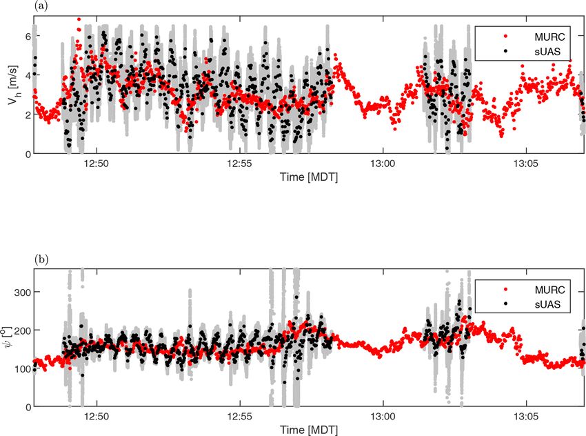
174                           L. Al-Ghussain and S. C. C. Bailey: Minimizing aircraft motion bias in wind measurements

et al., 2016). Wind velocity measurements can typically be         small errors in calibration and probe alignment (Suomi and
partitioned into several approaches: directly by using the in-     Vihma, 2018; Laurence and Argrow, 2018). Furthermore,
strumentation employing an onboard wind sensor and sub-            accurate position and orientation determination usually re-
tracting the aircraft kinematics (Suomi and Vihma, 2018;           quires very accurate orientation information (e.g., obtained
Cassano et al., 2016); indirectly using the attitude and po-       through the use of dual-antenna combination GPS–IMU),
sition data recorded by the inertial measurement unit (IMU)        and accurate time stamping of the data is critical to align
and GPS, respectively (Suomi and Vihma, 2018); using both          sensor and flight data. Here, we present an approach which
techniques (Rautenberg et al., 2018); or through calibration       can be implemented a posteriori to minimize the impact of
of the aircraft’s kinematic and dynamic response to the wind       unidentified and unquantified biases introduced during wind
(González-Rocha et al., 2020).                                     velocity measurement which result in contamination of the
   Broadly speaking, wind measurements taken by sensors            wind signal by the aircraft velocity. This contamination re-
like sonic anemometers, single- and multi-hole pressure            sults in overestimation or underestimation of the wind vector
probes, and hot wires tend to have higher temporal (and            and, in particular, errors in estimation of turbulence statistics
hence spatial) response (Suomi and Vihma, 2018). Multi-            (e.g., momentum fluxes, dissipation rate, turbulence kinetic
hole pressure probes have been frequently used for sUAS-           energy) measured by the sUAS. Hence, it is vital to mini-
based wind velocity measurements (van den Kroonenberg              mize errors in the wind components measured by sUASs. In
et al., 2008; Elston et al., 2015; Spiess et al., 2007; Thomas     the following sections we overview a multi-hole probe im-
et al., 2012) due to their high sampling frequency, light          plementation and discuss the potential sources of bias within
weight, simplicity, accuracy and almost linear relation be-        the approach. We then present a simple automated optimiza-
tween pressure and velocity at large flow velocities (Suomi        tion which is designed to identify and remove these biases
and Vihma, 2018). More importantly, multi-hole probes are          and demonstrate that this approach improves the wind esti-
able to resolve all three wind velocity components. The sim-       mate of an existing dataset.
plest multi-hole probe capable of resolving all three velocity
components is the five-hole probe, composed of five holes
arranged symmetrically on a semi-spherical or conical tip.         2   Multi-hole probe implementation
When the wind velocity is oriented in different directions rel-
                                                                   Multi-hole probes are an adaptation of the common Pitot
ative to the probe axis, each hole converts a different propor-
                                                                   static probe to allow the determination of relative wind di-
tion of the dynamic pressure to stagnation pressure, allowing
                                                                   rection and magnitude. Widely used in laboratory wind tun-
the dynamic pressure and direction to be determined using
                                                                   nel studies of three-dimensional flow fields, they found use
laboratory or in-flight calibration of the probe’s directional
                                                                   in manned aircraft studies of atmospheric wind (Treaster and
response.
                                                                   Yocum, 1978; Axford, 1968; Lenschow, 1972) before being
   The use of five-hole probes in sUAS measurements has
                                                                   adopted for sUAS use. Five-hole probes, being the simplest
evolved from their employment in manned aircraft mea-
                                                                   form of multi-hole probes, are most common. The arrange-
surements (Lenschow, 1970, 1972). Such measurements fre-
                                                                   ment of the normal vector of each plane of the holes on the
quently employ in-flight calibration procedures. For instance,
                                                                   probe tip typically consists of a central hole with normal vec-
Parameswaran and Jategaonkar (2004) presented a calibra-
                                                                   tor in line with the probe axis, measuring pressure P1 , and
tion procedure for five-hole probes using flight recorder data
                                                                   with the normal vector of the remaining holes at an angle to
with an optimization algorithm to estimate the time delay,
                                                                   the probe axis. Two holes measure the pressure at opposing
biases and scale factors in the pressure measurements. Af-
                                                                   directions on the horizontal plane, e.g., P2 and P3 , with the
terwards, the corrected five-hole probe measurements were
                                                                   remaining two in opposite directions on the vertical plane,
compared with the measurements from the inertial measure-
                                                                   e.g., P4 and P5 . Static pressure, Ps , is also measured, either
ment unit to check their compatibility. Drüe and Heinemann
                                                                   through a ring of holes oriented perpendicular to the probe
(2013) present a comprehensive review of in-flight calibra-
                                                                   axis or through an alternate pressure port. Wind tunnel cal-
tion of several atmospheric measurement instruments, in-
                                                                   ibrations are used to determine calibration coefficients, for
cluding five-hole probes. They identified five-hole probe in-
                                                                   example
flight calibration maneuvers to determine the sideslip angle,
angle of attack, static pressure and position errors. More-        CPyaw = (P2 − P3 )/(P1 − P ) ,                               (1)
over, they highlighted the need for in-flight calibration in the
                                                                   CPpitch = (P2 − P5 )/(P1 − P ) ,                             (2)
experiment location under favorable atmospheric conditions
and following removal of the sensors from the aircraft.            CPtotal = (P1 − P0 )/(P1 − P ) ,                             (3)
   The simplicity and compact nature of multi-hole probes          P = (P2 + P3 + P4 + P5 )/4 ,                                 (4)
also make it particularly useful for fixed-wing sUASs. How-
ever, as with manned aircraft, these aircraft have the ability     where P0 = 0.5ρ|U m |2 + Ps is the total pressure, ρ the den-
to fly at velocities up to an order of magnitude greater than      sity of the air and |U m | the magnitude of the relative air
the wind velocity, and their usage can be very sensitive to        velocity vector U m . During calibration P1 , P2 , P3 , P4 , P5

Atmos. Meas. Tech., 14, 173–184, 2021                                                 https://doi.org/10.5194/amt-14-173-2021
L. Al-Ghussain and S. C. C. Bailey: Minimizing aircraft motion bias in wind measurements                                          175

and Ps are measured at different sideslip, β, and angle of           of gravity, that r is precisely known, that there are negligible
attack, α, at known P0 . Depending on the specifics of the           flow blockage effects in the wind tunnel calibration or from
probe geometry, a unique set of coefficients is recovered for        the aircraft fuselage, and that all sensors are free of error. Al-
each α and β combination up to some limit (referred to as the        though every effort can be made to minimize these biases, it
cone angle) typically between 25 and 45◦ depending on the            is unlikely that they can be removed completely. The result
specifics of the probe geometry. During measurement P1 , P2 ,        is that U is often contaminated by U s . This is most evident
P3 , P4 , P5 and Ps are simultaneously sampled and CPyaw and         when LBI , U ac and  are changing rapidly. The following
CPpitch calculated for each sample. The known dependence of          section describes a procedure developed to determine addi-
α, β and CPtotal on CPyaw and CPpitch from the calibration is        tional calibration coefficients and implement them following
then applied to determine α, β and P0 , which, when com-             an in-flight calibration or measurement to minimize these bi-
bined with a known ρ, provide the air velocity and direction         ases.
relative to the probe axis. Additional calibration is also pos-
sible to account for an imprecise frequency response of the
probes caused by resonance and viscous damping in the pres-          3   Correction procedure
sure tubing and sensors (e.g., as described in Gerstoft and
Hansen, 1987), which can potentially require additional cor-         The net effect of the majority of biases can be summarized
rections (e.g., Yang et al., 2006). These additional corrections     as influencing four parameters. Misalignment of probe and
are not addressed here.                                              aircraft axes, calibration errors, and aerodynamic distortion
   When implemented on a moving platform such as an air-             of the flow around the probe will introduce bias errors into
craft, U m is no longer the wind velocity but is instead a com-      the time-dependent pitch, roll and yaw angles θ (t), φ(t) and
bination of the aircraft and wind velocity vectors:                  γ (t), which relate the measured velocity vector in body-
                                                                     frame coordinates to the aircraft velocity vector. In addi-
[U m ]B = [U ]B − [U s ]B ,                                   (5)    tion, calibration errors, transducer errors and airframe aero-
                                                                     dynamic effects (e.g., airframe blockage and streamline de-
where U s is the velocity vector of the sensor and U is the de-
                                                                     flection due to the generation of lift) can also influence the
sired wind velocity vector. We have also introduced the sub-
                                                                     direction of airflow relative to the probe and the magnitude
script B to indicate that these velocities are in a body-fixed
                                                                     of the measured dynamic pressure Q(t) = 0.5ρ(t)|U m (t)|2
frame of reference, i.e., a coordinate system attached to the
                                                                     relative to the true dynamic pressure. Note that the distortion
aircraft. Due to the pitch, roll and yaw angles of the aircraft,
                                                                     of the flow may also depend on lift production of the aircraft
 = [θ φ γ ], or more specifically their time rate of change
 ˙ U s can experience additional velocity relative to the air-       and therefore Q(t) may also include dependence on the lift
,
                                                                     coefficient, which is not considered in the version of the cor-
craft velocity U ac = [Uac Vac Wac ] (Lenschow and Johnson,
                                                                     rections described here. Finally, it is also important for all
1968) such that
                                                                     sensor readings to precisely correspond to orientation read-
                      ˙ × r]B ,
[U s ]B = [U ac ]B + [                                       (6)    ings in time to allow precise removal of aircraft motion from
                                                                     measured relative air velocity. However, implementation of
where r is the distance vector between the aircraft center of        software and differences in sensor time response can cause
gravity and the measurement volume on the probe.                     a delay between when probe-measured velocity and aircraft-
   Note that the desired quantity is [U ]I = [U V W ], the           measured velocity occur; e.g., the values of U m (t) and U s (t)
wind velocity vector in the Earth-fixed inertial frame of ref-       may not correspond to the same t. The proposed correction
erence. Furthermore, U ac is also typically measured in the          procedure assumes that these values are biased in a way such
Earth-fixed inertial frame (e.g., through a global positioning       that
system), and therefore a transformation matrix LBI must be
determined using the aircraft’s pitch (θ ), roll (φ) and yaw (γ )    θ (t) = θm (t) + 1θ,                                          (7)
angles in the inertial frame. The velocity vector [U ac ]I , along   φ(t) = φm (t) + 1φ,                                           (8)
with θ , φ, γ and their rates as required to build  and LBI ,
                                                                     γ (t) = γm (t) + 1γ ,                                         (9)
can be measured by an onboard inertial measurement unit
and GPS, and they are commonly provided by most autopi-              Q(t) = ζ Qm (t),                                             (10)
lots used for sUAS operation, thus providing enough infor-           U m (t) = U m (tm + 1t),                                     (11)
mation to determine [U ]I from [U m ]B .
   However, as noted earlier, U s is often an order of magni-        where the subscripted m indicates the measured value. The
tude larger than the desired U , making the process sensitive        objective is then to find 1 = {1θ, 1φ, 1γ , ζ, 1t}. Using
to an abundance of small biases. For example, the procedure          assumptions about how these biases will impact U (t) allows
above assumes perfect alignment between the probe’s coor-            the determination of optimal values for 1 which minimize
dinate system and the aircraft’s coordinate system. It also as-      this negative behavior. With 1 known, we are able to re-
sumes that  and LBI are measured at the aircraft’s center           move its influence on the final time series of U (t).

https://doi.org/10.5194/amt-14-173-2021                                                     Atmos. Meas. Tech., 14, 173–184, 2021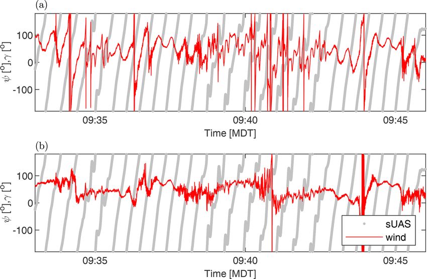
176                            L. Al-Ghussain and S. C. C. Bailey: Minimizing aircraft motion bias in wind measurements

   The assumptions used here are relatively straightforward,          flight trajectory. For flight trajectories without many trajec-
the first being that any biasing of U (t) by U s will result in       tory changes, it was also found that the objective function
U (t) having a dependence on the direction of travel of the
aircraft. The second assumption we make is that the vertical          δ = h(U − hU i)2 i + h(V − hV i)2 i                         (15)
component of U (t) will be approximately zero in the mean.
                                                                      was equally effective, but it relies on the assumption that the
This assumption may not hold in flight over sloped terrain
                                                                      biases will act only to increase the fluctuations of the velocity
and/or for relatively short flight domains (both spatial and
                                                                      signal at the probe. Here h i indicates an average over the en-
temporal), in which case an alternative assumption may be
                                                                      tire portion of the flight used to find 1. The resulting value
needed. Moreover, we assume that the sensors have an ade-
                                                                      of 1t which minimizes δ is then implemented in the remain-
quate response and that the greatest error is due to the spe-
                                                                      ing optimization stages.
cific configuration which logs IMU–GPS, pressure transduc-
                                                                         The second stage follows a similar approach. Noting that
ers, and local pressure, temperature and humidity (PTU) on
                                                                      the mean value of the vertical component of [U (t)]I , i.e.,
three separate systems.
                                                                      W (t), is most sensitive to 1θ , we then find the value of 1θ
   The correction procedure, as implemented, follows a mul-
                                                                      that minimizes
tistage approach used to optimize 1. This multistage ap-
proach was implemented to allow different objective func-             δ = hW i                                                    (16)
tions to be used for different components of 1. However,
in practice, it is likely that a well-implemented single-stage        using U m (t) = U m (tm + 1t) as found above.
optimization will achieve the same results.                              The remaining elements of 1, specifically ζ , 1φ and
   The first step is to identify a portion of the flight which will   1γ , are then found by minimizing δ as defined in Eq. (14)
be used to determine 1. This portion should not include any          using U m (t) = U m (tm + 1t) and θ = θm + 1θ as found in
significant acceleration or deceleration of the aircraft’s hor-       the preceding two stages.
izontal ground speed (e.g., as experienced during takeoff or             Finally, to ensure that the values of 1 determined us-
landing) and should include multiple changes of direction of          ing the latter optimization stages do not influence the values
the aircraft. In addition, the portion should be long enough          found during the earlier stages, 1 is further refined by re-
to ensure that unsteadiness in the mean winds, e.g., as in-           peating the above three stages once again. In practice, this
troduced by thermals, are averaged out. Ideally, devoting a           last step only influenced 1 by 1 % or less and can likely be
portion of the flight after takeoff to conducting calibration         omitted without loss of confidence in the final values of 1.
orbits for later use in this process would be desired. With
this portion of the flight identified, the determination of 1
                                                                      4     Results
is found by an optimization process seeking to minimize an
objective function, δ, through iterative calculation of [U ]I (as     With 1 known, the biases described by 1 can be removed
described in Sect. 2).                                                following Eqs. (7) to (11) prior to a final determination of
   Through perturbing 1 and examining its influence on               [U (t)]I . To validate this correction procedure, we applied
U (t) it was found that the standard deviation of the horizon-        it to measurement data acquired during the LAPSE-RATE
tal components of [U (t)]I , specifically U (t) and V (t), were       campaign described in de Boer et al. (2018). The data were
most sensitive to 1t (due to the aircraft flight being predom-        acquired using two different five-hole-probe-equipped fixed-
inantly in the horizontal plane), with values of 1t as low            wing aircraft, with the aircraft, probe and data reduction pro-
as tenths or hundredths of a second contributing to large bi-         cedures described in detail in Witte et al. (2017). We first
ases of the horizontal components of [U (t)]I . We thus first         demonstrate the correction procedure in flights compared to
use a Nelder–Mead multidimensional unconstrained nonlin-              a ground reference, followed by a demonstration of the im-
ear minimization approach, implemented using the MAT-                 provements made to vertical profiles of the wind velocity and
LAB fminsearch command, to identify the value of 1t which             direction.
minimizes the objective function δ, defined as
                                                                      4.1    Comparison to ground reference
δU = hU i|Uac >0 − hU i|Uac 0 − hV i|Uac 0 indicates an average conditioned on when         detailed in Barbieri et al. (2019), the intercomparison was
the aircraft is flying with a positive inertial velocity compo-       conducted by flying the sUASs near the Mobile UAS Re-
nent Uac . Likewise, h i|Uac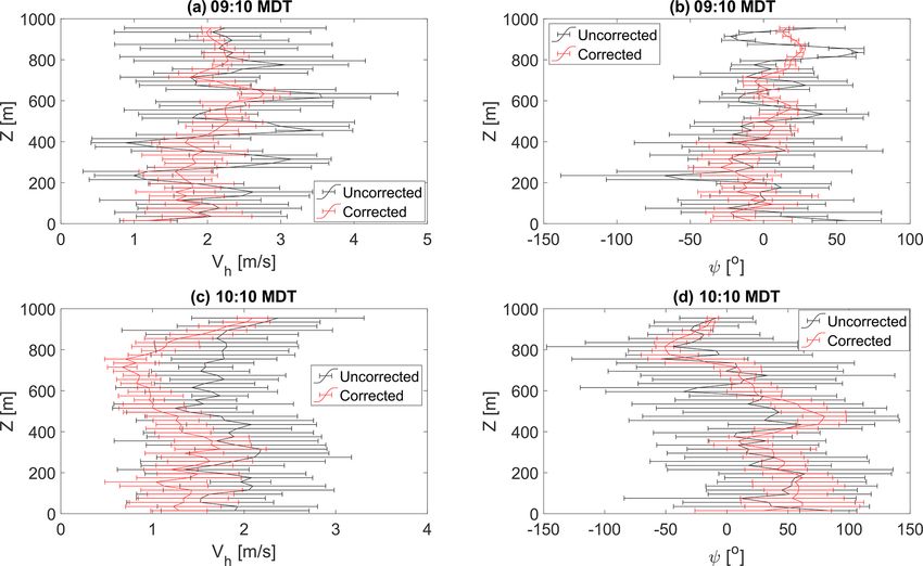
L. Al-Ghussain and S. C. C. Bailey: Minimizing aircraft motion bias in wind measurements 177
the mast at 20 m above ground level with an orbit radius of reference sensor were not collocated. Also shown as a dashed
80 m. This orbit was performed for approximately 5 min be- line in the figure are the bounds described by 2 standard de-
fore the aircraft ascended to 120 m to perform similar orbits viations of the difference between the sUAS- and MURC-
for 2 min, then descending back to 20 m to resume the orbits measured values.
around the tower for another 2 min before starting its landing For the uncorrected velocity magnitude and direction, the
pattern. comparison shown in Figs. 4a and b reveals a broad spread
This circular flight pattern introduced a periodic variation about the reference line. This spread decreases significantly
in θ , γ and φ, with the period corresponding to the time when the corrections are applied, as shown by comparison to
to complete an orbit (approximately 25 s). Although conve- Figs. 4c and d. The mean difference between the two mea-
nient for the measurement of atmospheric parameters at a surements decreases by approximately 35 % in magnitude
single geographic location, these types of orbits consist of the and direction with correction, corresponding to an increase
worst-case scenario for the contamination of the measured in the correlation coefficient from 0.13 to 0.19 in magnitude
wind direction by the biases discussed in Sect. 2. and 0.22 to 0.32 in direction. This increased correlation is
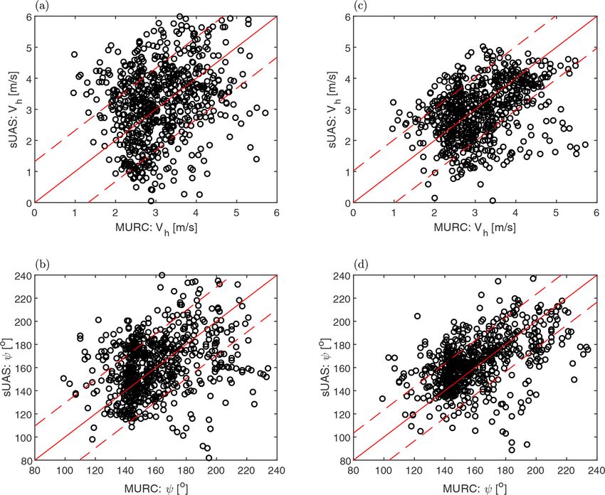
The periodicity is clearly evident in the estimated horizon- reflected in the statistics. The correction brings the standard
tal wind speed, Vh = (U 2 +V 2 )1/2 , and direction, ψ, prior to deviation of the sUAS-measured velocity much closer to the
implementing the corrections, as shown in Fig. 1a and b, re- reference signal. The standard deviation in magnitude mea-
spectively. Although the general trends of the measured wind sured by the sUAS decreases from 1.2 to 0.90 m s−1 , very
velocity and direction time series follow that of the reference close to the value of 0.86 m s−1 measured by the reference.
velocity and direction, the magnitude of the fluctuations is For direction the standard deviation decreases with correc-
clearly contaminated by the aircraft velocity and direction. tion from 27 to 22◦ , whereas it is 24◦ for the reference.
The period in the wind signal is consistent with the time re-
quired to orbit the fixed mast at 25 s. Note that in Fig. 1 only 4.2 Implementation in profiling measurements
the two portions of the flight during which the sUAS is at the
same altitude as the reference sensors are presented. The results of the comparison to the ground reference pro-
The same time series are shown in Fig. 2a and b vide confidence in the success of the correction. To demon-
corrected following the procedure described in Sect. 3. strate the improvement offered by application of these cor-
The 10 min of flight between 12:49 and 12:58 MDT were rections to vertical profiling by fixed-wing aircraft, we now
selected to conduct the optimization of 1. The result examine their impact on profiles of wind speed and direc-
of optimization was 1 = {1θ = −6.4◦ , 1φ = 0.9◦ , 1γ = tion measured by two separate aircraft at different locations.
2.1◦ , ζ = 1.07, 1t = −0.045 s}, which highlights the sensi- These two fixed-wing aircraft were essentially identical in
tivity of the estimated wind velocity and direction to even configuration to that described in Witte et al. (2017) and were
small deviations from ideal orientations. As shown in Fig. 2, flown at measurement sites separated by 16 km. Each aircraft
the corrected signals are now largely free of the 25 s period- measured an atmospheric profile every hour, with the two air-
icity, although there is some evidence of contamination be- craft staggered in time by 30 min.
tween 12:56 and 12:58 MDT. When the aircraft returns to Each profile consisted of a 20 min flight, with the aircraft
18 m of altitude for the second set of orbits (which were not performing a spiralling ascent to 900 m followed by a spi-
included in the optimization) there is little evidence of air- ralling descent, with this pattern repeated until the 10Ah
craft velocity contamination in the wind estimates. battery was depleted. In the following discussion the times
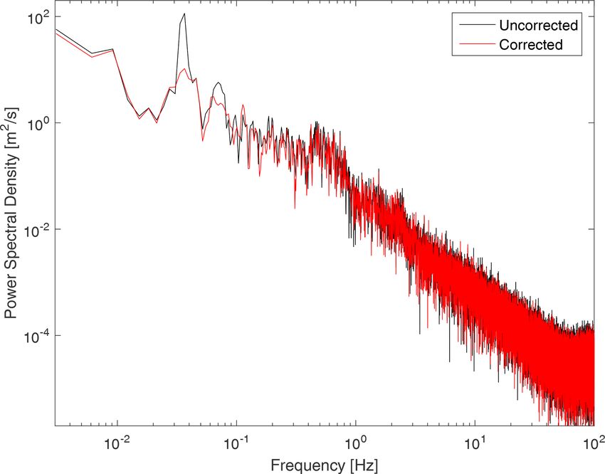
The periodicity described above is more clearly evident are those corresponding to when the profile measuring flight
in the difference between the power spectrum of horizontal initiates with the X, Y and Z coordinate system origin at
wind speed calculated for both the corrected and uncorrected the takeoff location. These particular profiles were selected
cases. These spectra are presented in Fig. 3. The influence for discussion as they were measured during the boundary
of the periodic orbits of the aircraft is apparent in the uncor- layer transition and represent different behaviors, including
rected measurements as a spike at 0.035 Hz (consistent with the presence of turbulence and variability in the wind direc-
an orbital period of 28 s). This spike is greatly reduced by tion. The wind speeds during these profiles were also low,
the correction. Importantly, besides what appears to be a har- producing a large ratio of aircraft velocity to wind veloc-
monic peak at 0.07 Hz which is also reduced, the remainder ity and therefore a challenging case to accurately extract the
of the spectrum appears largely unaffected by the correction. wind components from the five-hole probe signal.
To provide a more quantitative comparison between the As previously mentioned, the orbital flight patterns also
sUAS and reference measurement, we directly compare the represented a challenge for extracting the wind data due to
velocity magnitude and direction measured at each instant a the periodic variation in θ , γ and φ introducing a correspond-
sample was made by the ground reference. This comparison ing periodic variation in [U (t)]I . This bias can be clearly il-
is presented in Fig. 4 in which a perfect comparison would lustrated by comparing γ to ψ, as done for an example flight
result in the straight line as indicated in the figure. Note that, in Fig. 5a. For this flight, the aircraft completed a full 360◦
a perfect correlation should not be expected as the sUAS and turn in approximately 30 s, introducing a corresponding pe-
https://doi.org/10.5194/amt-14-173-2021 Atmos. Meas. Tech., 14, 173–184, 2021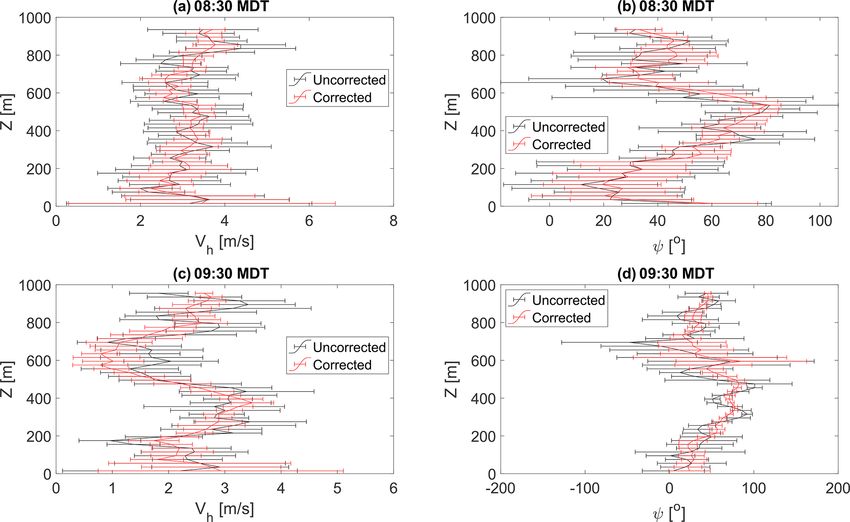
178                             L. Al-Ghussain and S. C. C. Bailey: Minimizing aircraft motion bias in wind measurements

Figure 1. Comparison between uncorrected (a) horizontal wind speed and (b) wind direction measured by the sUAS to the reference signal
measured by MURC. Gray lines indicate full signal from the sUAS, whereas black lines indicate the same signal downsampled to the same
data rate as that of the MURC by plotting every 200th data point.

Figure 2. The sUAS-based wind measurements from Fig. 1 following correction compared to the reference signal measured by MURC:
(a) horizontal wind speed and (b) wind direction. Gray lines indicate full signal from the sUAS, whereas black lines indicate the same signal
downsampled to the same data rate as that of the MURC by plotting every 200th data point.

Atmos. Meas. Tech., 14, 173–184, 2021                                                        https://doi.org/10.5194/amt-14-173-2021
L. Al-Ghussain and S. C. C. Bailey: Minimizing aircraft motion bias in wind measurements                                       179

                                                                   Table 1. Components of 1 determined by optimization for each
                                                                   sUAS for both flights.

                                                                    sUAS     Flight        1θ      1φ       1γ       ζ    1t
                                                                    1        08:30 MDT     −4.9◦   0.17◦    2.6◦    1.1   0.98 s
                                                                    1        09:30 MDT     −5.8◦   2.7◦     2.1◦    1.1   0.01 s
                                                                    2        09:10 MDT     −3.9◦   0.85◦    1.4◦   1.15   2.9 s
                                                                    2        10:10 MDT     −3.9◦   0.78◦    1.3◦   1.15   2.6 s

                                                                   noticeably stronger velocity and direction fluctuations mea-
                                                                   sured for Z < 200 m, indicating the presence of turbulence
                                                                   near the surface. This turbulence appears to still have been
                                                                   present at 09:30 MDT, as shown in Fig. 6c and d, but at this
                                                                   time there was a region of calm air centered at Z = 600 m,
Figure 3. Power spectrum of horizontal wind magnitude calculated
from uncorrected and corrected time series.
                                                                   coinciding with a significant deviation in measured wind di-
                                                                   rection. For Z > 200 m, the corrected profile of wind direc-
                                                                   tion was consistent with the one measured at 08:30 MDT, ex-
                                                                   cept the region of calm air at Z = 600 m.
riod in both the wind speed and direction before correction.          At the site measured by sUAS 2, the corrected mean
Once the corrections have been applied, as shown in Fig. 5b,       wind speed and direction profiles measured at 09:10 MDT
there is a distinct reduction of periodicity in the direction of   shown in Fig. 7a and b reflect a boundary layer undergo-
the wind measured by the sUAS.                                     ing transition, with evidence of turbulence for Z < 500 m.
   The means of the corresponding wind speed and direction         At 10:10 MDT, as shown in Fig. 7c and d, a multi-layer
profiles are presented in Fig. 6 for sUAS 1 and Fig. 7 for         structure was also evident in the wind profiles in the form
sUAS 2. In these figures both the uncorrected and corrected        of significant changes in the wind direction throughout the
mean profiles are displayed in order to show the relative im-      profile. The horizontal wind speed was relatively consistent
provement offered by application of the bias correction. For       between 1 and 2 m s−1 for Z < 800 m, but there was evi-
all profiling flights, the correction coefficients were deter-     dence of stronger turbulence for Z < 500 m and moderate
mined by optimizing the entire flight once the aircraft was        wind shear for Z > 700 m. As noted, the wind direction ex-
in its flight pattern. Before correction, the bias introduced      hibited significant variation in the range 400 m < Z < 500 m,
by the aircraft trajectory is apparent as large coherent devi-     with continual backing within 500 m < Z < 900 m and veer-
ations from the general trend, mostly evident in the velocity      ing for Z < 900 m. These different altitudes of behavior were
magnitude but also present in the direction. When the cor-         consistent with the measured potential temperature changes
rections were applied, these large deviations were greatly         (not included for conciseness) and became much easier to
reduced, better representing the structure of the boundary         identify in the corrected profiles than they were before cor-
layer throughout the profiles. In the wind velocity profiles       rection.
presented in Fig. 6 for sUAS 1 there were still high veloc-           It is clear through comparison of the corrected and uncor-
ity deviations, even in the corrected profiles near the sur-       rected profiles in Figs. 6 and 7 that the corrections reduce
face corresponding to when the aircraft was being manually         fluctuations about the mean profile under different condi-
controlled and experiencing strong acceleration. It has been       tions and for different aircraft. Similar improvements have
found that the corrections presented here cannot completely        been observed for other profiles measured with these and
remove the bias due to aircraft acceleration, suggesting a po-     other sUASs. The coefficients determined by the optimiza-
tential time response lag between the five-hole probe and the      tion routine for these profiles are presented in Table 1. Com-
inertial measurement unit, which agrees with what was re-          paring each flight for the same sUAS demonstrates that the
ported in Båserud et al. (2016).                                   automated optimization converged on nearly identical coeffi-
   The corrected profiles show very different wind behav-          cients for the same sUAS, with only one coefficient changing
iors for the different sites and times. At the site measured       by more than 1◦ between each flight. Indeed, the correction
by sUAS 1, the profiles measured at 08:30 MDT shown in             coefficients were found to be remarkably similar for each
Fig. 6a and b reflect the correspondence between the stable        sUAS used throughout the LAPSE-RATE campaign. This
thermodynamic conditions throughout the boundary layer             similarity between the coefficients reinforces the assumption
and the horizontal wind magnitude, with winds increasing           that the biases are caused by physical misalignment between
from 2 m s−1 near the ground to 4 m s−1 at Z = 900 m and           the coordinate systems of the aircraft and the five-hole probe.
staying consistently between ψ = 0◦ and 100◦ . There was           Note that bias corrected by 1t should not be expected to be

https://doi.org/10.5194/amt-14-173-2021                                                Atmos. Meas. Tech., 14, 173–184, 2021
180 L. Al-Ghussain and S. C. C. Bailey: Minimizing aircraft motion bias in wind measurements Figure 4. Direct comparison between (a) uncorrected and (c) corrected horizontal wind speed measured simultaneously by the sUAS and MURC. Similar comparison shown for (b) uncorrected and (d) corrected wind direction. The solid red line indicates where both measure- ments are identical, and dashed lines indicate 2 standard deviations of the difference between the sUAS- and MURC-measured values. Figure 5. Comparison between measured wind direction and aircraft yaw direction for (a) uncorrected and (b) corrected signals as a function of time for a single flight. Atmos. Meas. Tech., 14, 173–184, 2021 https://doi.org/10.5194/amt-14-173-2021
L. Al-Ghussain and S. C. C. Bailey: Minimizing aircraft motion bias in wind measurements                                         181

Figure 6. Comparison of mean (a) horizontal wind magnitude and (b) wind direction profiles measured by sUAS 1 at 08:30 MDT with and
without correction applied. Horizontal mean magnitude and direction profiles measured at 09:30 MDT are shown in (c, d), respectively.

Figure 7. Comparison of mean (a) horizontal wind speed and (b) direction profiles measured by sUAS 2 at 09:10 MDT with and without
correction applied. Horizontal wind speed and direction profiles measured at 10:10 MDT are shown in (c, d), respectively.

https://doi.org/10.5194/amt-14-173-2021                                                  Atmos. Meas. Tech., 14, 173–184, 2021
182                             L. Al-Ghussain and S. C. C. Bailey: Minimizing aircraft motion bias in wind measurements

consistent for the systems used here, as the time series of U m ,      for each five-hole probe. Processing the raw data requires numer-
U ac and  are measured by separate acquisition systems at             ous customized scripts and configuration files to convert the raw
different rates and aligned using post-processing software.            voltages to relative velocity, align the data files in time, and extract
Thus, the 1t bias is most likely introduced by errors in this          the wind speed from the relative velocity. Given the level of cus-
alignment process and can be expected to be random.                    tomization to the specific instruments used within these codes, it
                                                                       was not felt that providing the raw data and codes would provide
                                                                       value to the community. Interested parties are welcome to contact
                                                                       the corresponding author to request access to these files.
5   Conclusions

Small unmanned aerial systems have been increasingly used
                                                                       Author contributions. SCCB conceived the correction, which was
in atmospheric research. Frequently, this research requires            implemented by LAG. Both authors contributed to paper prepara-
the acquisition of the wind velocity vector. Multi-hole probe          tion.
measurements are among the more common and reliable
techniques used for this purpose. However, when imple-
mented on sUASs there is significant potential to introduce            Competing interests. The authors declare no competing interests.
bias due to the large ratio of aircraft velocity to the wind ve-
locity. Therefore, the measured wind velocities are very sen-
sitive to these small biases. Furthermore, when conducting             Acknowledgements. This work was supported by the National Sci-
vertical profiles at a fixed location, these profiles typically        ence Foundation through grant no. CBET-1351411 and award no.
require circular flight patterns, which increase the probabil-         1539070: Collaboration Leading Operational UAS Development
ity of small misalignment between the probe and the air-               for Meteorology and Atmospheric Physics (CLOUDMAP). The au-
craft axes, introducing a time-dependent periodic error in             thors would like to thank Caleb Canter, Jess Estridge, Jonathan
the wind velocity measurement that can propagate into post-            Hamilton, Sean MacPhee, Ryan Nolin, Isaac Rowe, Christopher
flight analysis such as the calculation of energy spectra and          Saunders, Virginia Smith, Christina Vezzi and Harrison Wight, who
                                                                       maintained and flew the aircraft used in this study, as well as cali-
Reynolds stresses.
                                                                       brating and manufacturing the probes.
   An approach was presented that can be applied in post-
processing of the flight data to automatically estimate the bi-
ases in axis misalignment and errors in their alignment in             Financial support. This research has been supported by the Na-
time. Once estimated, these biases can be removed, improv-             tional Science Foundation Division of Chemical, Bioengineering,
ing the quality of the wind estimate.                                  Environmental, and Transport Systems (grant no. CBET-1351411)
   These corrections were validated using data acquired as             and the National Science Foundation Office of Experimental Pro-
part of the LAPSE-RATE field campaign. Measurements                    grams to Stimulate Competitive Research (award no. 1539070).
flown near a ground-based reference system revealed a sig-
nificant reduction in measured oscillations of both wind mag-
nitude and direction, which corresponded to the aircraft flight        Review statement. This paper was edited by Laura Bianco and re-
pattern. Additional verification was conducted by comparing            viewed by William Thielicke and two anonymous referees.
profiles of wind speed and direction measured by two differ-
ent aircraft at two different times. The estimated biases were
within ±1◦ for each aircraft, and successful minimization of
aircraft-induced oscillations in the measured profiles was ob-
                                                                       References
served for both aircraft. These results confirm that the biases
are most likely due to physical misalignment of the aircraft           Axford, D. N.: On the Accuracy of Wind Measurements Us-
and probe axes, as well as demonstrating that the same cor-              ing an Inertial Platform in an Aircraft, and an Example of a
rection procedures can be applied to multiple aircraft.                  Measurement of the Vertical Mesostructure of the Atmosphere,
                                                                         J. Appl. Meteorol., 7, 645–666, https://doi.org/10.1175/1520-
                                                                         0450(1968)0072.0.CO;2, 1968.
Data availability. Corrected data presented in this paper are          Bailey, S. C. C., Canter, C. A., Sama, M. P., Houston,
openly available in the Zenodo LAPSE-RATE community data                 A. L., and Smith, S. W.: Unmanned aerial vehicles re-
repository (https://zenodo.org/communities/lapse-rate/, last access:     veal the impact of a total solar eclipse on the atmospheric
23 July 2020), with the University of Kentucky data available at         surface layer, P. Roy. Soc. A-Math Phy., 475, 20190212,
https://doi.org/10.5281/zenodo.3701845 (Bailey et al., 2020). Test-      https://doi.org/10.1098/rspa.2019.0212, 2019.
ing the correction described in this paper requires processing the     Bailey, S. C. C., Smith, S. W., and Sama, M. P.: Univer-
raw data to produce wind vector estimates consisting of raw volt-        sity of Kentucky files from LAPSE-RATE, Data set, Zenodo,
age data from the five-hole probe, pressure, temperature and hu-         https://doi.org/10.5281/zenodo.3701845, 2020.
midity from the iMet sensor, and 6 DOF (degrees of freedom) data       Balsley, B. B., Lawrence, D. A., Woodman, R. F., and Fritts, D. C.:
from the IMU–GPS system as well as individual calibration files          Fine-scale characteristics of temperature, wind, and turbulence in

Atmos. Meas. Tech., 14, 173–184, 2021                                                       https://doi.org/10.5194/amt-14-173-2021
L. Al-Ghussain and S. C. C. Bailey: Minimizing aircraft motion bias in wind measurements 183
the lower atmosphere (0–1,300 m) over the south Peruvian coast, Drüe, C. and Heinemann, G.: A review and practical guide to
Bound.-Lay. Meteorol., 147, 165–178, 2013. in-flight calibration for aircraft turbulence sensors, J. Atmos.
Barbieri, L., Kral, S. T., Bailey, S. C. C., Frazier, A. E., Jacob, J. Ocean. Tech., 30, 2820–2837, https://doi.org/10.1175/JTECH-
D., Reuder, J., Brus, D., Chilson, P. B., Crick, C., Detweiler, C., D-12-00103.1, 2013.
Doddi, A., Elston, J., Foroutan, H., González-Rocha, J., Greene, Egger, J., Bajrachaya, S., Heingrich, R., Kolb, P., Lammlein, S.,
B. R., Guzman, M. I., Houston, A. L., Islam, A., Kemppinen, Mech, M., Reuder, J., Schäper, W., Shakya, P., Shween, J., and
O., Lawrence, D., Pillar-Little, E. A., Ross, S. D., Sama, M. Wendt, H.: Diurnal Winds in the Himalayan Kali Gandaki Valley.
P., Schmale, D. G., Schuyler, T. J., Shankar, A., Smith, S. W., Part III: Remotely Piloted Aircraft Soundings, Mon. Wea. Rev.,
Waugh, S., Dixon, C., Borenstein, S., and de Boer, G.: Intercom- 130, 2042–2058, 2002.
parison of Small Unmanned Aircraft System (sUAS) Measure- Elston, J., Argrow, B., Frew, E., Houston, A., and Straka, J.: Evalu-
ments for Atmospheric Science during the LAPSE-RATE Cam- ation of unmanned aircraft systems for severe storm sampling
paign, Sensors, 19, 2179, https://doi.org/10.3390/s19092179, using hardware-in-the-loop simulations, J. Aeros. Comp. Inf.
2019. Com., 8, 269–294, 2011.
Bärfuss, K., Pätzold, F., Altstädter, B., Kathe, E., Nowak, S., Elston, J., Argrow, B., Stachura, M., Weibel, D., Lawrence, D., and
Bretschneider, L., Bestmann, U., and Lampert, A.: New setup Pope, D.: Overview of small fixed-wing unmanned aircraft for
of the UAS ALADINA for measuring boundary layer proper- meteorological sampling, J. Atmos. Ocean. Tech., 32, 97–115,
ties, atmospheric particles and solar radiation, Atmosphere, 9, 2015.
28, https://doi.org/10.3390/atmos9010028, 2018. Gerstoft, P. and Hansen, S.: A new tubing system for the measure-
Båserud, L., Reuder, J., Jonassen, M. O., Kral, S. T., Paskyabi, M. ment of fluctuating pressures, J. Wind Eng. Ind. Aerod., 25, 335–
B., and Lothon, M.: Proof of concept for turbulence measure- 354, https://doi.org/10.1016/0167-6105(87)90026-2, 1987.
ments with the RPAS SUMO during the BLLAST campaign, At- González-Rocha, J., De Wekker, S. F. J., Ross, S. D., and Woolsey,
mos. Meas. Tech., 9, 4901–4913, https://doi.org/10.5194/amt-9- C. A.: Wind profiling in the lower atmosphere from wind-
4901-2016, 2016. induced perturbations to multirotor UAS, Sensors, 20, 1341,
Bonin, T., Chilson, P., Zielke, B., and Fedorovich, E.: Observa- https://doi.org/10.3390/s20051341, 2020.
tions of the Early Evening Boundary-Layer Transition Using a Hobbs, S., Dyer, D., Courault, D., Olioso, A., Lagouarde, J.-P., Kerr,
Small Unmanned Aerial System, Bound.-Lay. Meteorol., 146, Y., McAnneney, J., and Bonnefond, J.: Surface layer profiles of
119–132, https://doi.org/10.1007/s10546-012-9760-3, 2013. air temperature and humidity measured from unmanned aircraft,
Calmer, R., Roberts, G. C., Preissler, J., Sanchez, K. J., Derrien, Agronomie, 22, 635–640, https://doi.org/10.1051/agro:2002050,
S., and O’Dowd, C.: Vertical wind velocity measurements us- 2002.
ing a five-hole probe with remotely piloted aircraft to study Illingworth, S., Allen, G., Percival, C., Hollingsworth, P., Gallagher,
aerosol–cloud interactions, Atmos. Meas. Tech., 11, 2583–2599, M., Ricketts, H., Hayes, H., Ładosz, P., Crawley, D., and Roberts,
https://doi.org/10.5194/amt-11-2583-2018, 2018. G.: Measurement of boundary layer ozone concentrations on-
Cassano, J. J., Maslanik, J. A., Zappa, C. J., Gordon, A. L., Cul- board a Skywalker unmanned aerial vehicle, Atmos. Sci. Lett.,
lather, R. I., and Knuth, S. L.: Observations of Antarctic polynya 15, 252–258, https://doi.org/10.1002/asl2.496, 2014.
with unmanned aircraft systems, Eos T. Am. Geophys. Un., 91, Jacob, J. D., Chilson, P. B., Houston, A. L., and Smith,
245–246, 2010. S. W.: Considerations for Atmospheric Measurements with
Cassano, J. J., Seefeldt, M. W., Palo, S., Knuth, S. L., Bradley, A. Small Unmanned Aircraft Systems, Atmosphere, 9, 252,
C., Herrman, P. D., Kernebone, P. A., and Logan, N. J.: Obser- https://doi.org/10.3390/atmos9070252, 2018.
vations of the atmosphere and surface state over Terra Nova Bay, Kral, S., Reuder, J., Vihma, T., Suomi, I., O’Connor, E.,
Antarctica, using unmanned aerial systems, Earth Syst. Sci. Data, Kouznetsov, R., Wrenger, B., Rautenberg, A., Urbancic, G.,
8, 115–126, https://doi.org/10.5194/essd-8-115-2016, 2016. Jonassen, M., Båserud, L., Maronga, B., Mayer, S., Lorenz, T.,
Cione, J., Kalina, E., Uhlhorn, E., Farber, A., and Damiano, B.: Holtslag, A., Steeneveld, G.-J., Seid, A., Müller, M., Linden-
Coyote unmanned aircraft system observations in Hurricane berg, C., Langohr, C., Voss, H., Bange, J., Hundhausen, M.,
Edouard (2014), Earth Space Sci., 3, 370–380, 2016. Hilsheimer, P., and Schygulla, M.: Innovative Strategies for Ob-
Corrigan, C. E., Roberts, G. C., Ramana, M. V., Kim, D., and servations in the Arctic Atmospheric Boundary Layer (ISO-
Ramanathan, V.: Capturing vertical profiles of aerosols and BAR) – The Hailuoto 2017 Campaign, Atmosphere, 9, 268,
black carbon over the Indian Ocean using autonomous un- https://doi.org/10.3390/atmos9070268, 2018.
manned aerial vehicles, Atmos. Chem. Phys., 8, 737–747, Laurence, R. J. and Argrow, B. M.: Development and flight test re-
https://doi.org/10.5194/acp-8-737-2008, 2008. sults of a small UAS distributed flush airdata system, J. Atmos.
de Boer, G., Ivey, M., Schmid, B., Lawrence, D., Dexheimer, D., Ocean. Tech., 35, 1127–1140, https://doi.org/10.1175/JTECH-
Mei, F., Hubbe, J., Bendure, A., Hardesty, J., Shupe, M. D., Mc- D-17-0192.1, 2018.
Comiskey, A., Telg, H., Schmitt, C., Matrosov, S. Y., Brooks, Lenschow, D.: The measurement of air velocity and tem-
I., Creamean, J., Solomon, A., Turner, D. D., Williams, C., perature using the NCAR Buffalo aircraft measuring sys-
Maahn, M., Argrow, B., Palo, S., Long, C. N., Gao, R.-S., tem, National Center for Atmospheric Research, Boulder,
and Mather, J.: A Bird’s-Eye View: Development of an Opera- Colorado, NCAR Technical Note, No. NCAR/TN-74+EDD,
tional ARM Unmanned Aerial Capability for Atmospheric Re- https://doi.org/10.5065/D6C8277W, 1972.
search in Arctic Alaska, B. Am. Meteorol. Soc., 99, 1197–1212, Lenschow, D. and Johnson, W.: Concurrent Airplane and Balloon
https://doi.org/10.1175/BAMS-D-17-0156.1, 2018. Measurments of Atmospheric Boundary Layer Structure Over A
Forest, J. Appl. Meteorol., 7, 79–89, 1968.
https://doi.org/10.5194/amt-14-173-2021 Atmos. Meas. Tech., 14, 173–184, 2021184 L. Al-Ghussain and S. C. C. Bailey: Minimizing aircraft motion bias in wind measurements Lenschow, D. H.: Airplane Measurements of Planetary Boundary Schuyler, T. J. and Guzman, M. I.: Unmanned Aerial Systems Layer Structure, J. Appl. Meteorol., 9, 874–884, 1970. for Monitoring Trace Tropospheric Gases, Atmosphere, 8, 206, Lothon, M., Lohou, F., Pino, D., Couvreux, F., Pardyjak, E. R., https://doi.org/10.3390/atmos8100206, 2017. Reuder, J., Vilà-Guerau de Arellano, J., Durand, P., Hartogensis, Shevchenko, A. M., Berezin, D. R., Puzirev, L. N., Tarasov, O., Legain, D., Augustin, P., Gioli, B., Lenschow, D. H., Faloona, A. Z., Kharitonov, A. M., and Shmakov, A. S.: Multi-hole I., Yagüe, C., Alexander, D. C., Angevine, W. M., Bargain, E., pressure probes to air data system for subsonic small-scale Barrié, J., Bazile, E., Bezombes, Y., Blay-Carreras, E., van de air vehicles, AIP Conference Proceedings, 1770, 030005, Boer, A., Boichard, J. L., Bourdon, A., Butet, A., Campistron, https://doi.org/10.1063/1.4963947, 2016. B., de Coster, O., Cuxart, J., Dabas, A., Darbieu, C., Deboudt, K., Spiess, T., Bange, J., Buschmann, M., and Vörsmann, P.: First appli- Delbarre, H., Derrien, S., Flament, P., Fourmentin, M., Garai, A., cation of the meteorological Mini-UAV ’M2AV’, Meteorol. Z., Gibert, F., Graf, A., Groebner, J., Guichard, F., Jiménez, M. A., 16, 159–169, https://doi.org/10.1127/0941-2948/2007/0195, Jonassen, M., van den Kroonenberg, A., Magliulo, V., Martin, S., 2007. Martinez, D., Mastrorillo, L., Moene, A. F., Molinos, F., Moulin, Suomi, I. and Vihma, T.: Wind gust measurement techniques E., Pietersen, H. P., Piguet, B., Pique, E., Román-Cascón, C., – From traditional anemometry to new possibilities, Sen- Rufin-Soler, C., Saïd, F., Sastre-Marugán, M., Seity, Y., Steen- sors (Switzerland), 18, 1–27, https://doi.org/10.3390/s18041300, eveld, G. J., Toscano, P., Traullé, O., Tzanos, D., Wacker, S., 2018. Wildmann, N., and Zaldei, A.: The BLLAST field experiment: Thomas, R. M., Lehmann, K., Nguyen, H., Jackson, D. L., Wolfe, Boundary-Layer Late Afternoon and Sunset Turbulence, Atmos. D., and Ramanathan, V.: Measurement of turbulent water va- Chem. Phys., 14, 10931–10960, https://doi.org/10.5194/acp-14- por fluxes using a lightweight unmanned aerial vehicle system, 10931-2014, 2014. Atmos. Meas. Tech., 5, 243–257, https://doi.org/10.5194/amt-5- Mansour, M., Kocer, G., Lenherr, C., Chokani, N., and Abhari, 243-2012, 2012. R. S.: Seven-Sensor Fast-Response Probe for Full-Scale Wind Treaster, A. L. and Yocum, A. M.: The calibration and application Turbine Flowfield Measurements, J. Eng. Gas Turb. Power, 133, of five-hole probes, Tech. rep., DTIC Document, 1978. 081601, https://doi.org/10.1115/1.4002781, 2011. van den Kroonenberg, A. C., Spieß, T., Buschmann, M., Mar- Parameswaran, V. and Jategaonkar, R. V.: Calibration of 5- tin, T., Anderson, P. S., Beyrich, F., and Bange, J.: Bound- hole probe for flow angles from advanced technologies test- ary layer measurements with the autonomous mini-UAV M2 AV, ing aircraft system flight data, Defence Sci. J., 54, 111–123, in: Deutsch–Österreichisch–Schweizerische Meteorologen – https://doi.org/10.14429/dsj.54.2073, 2004. Tagung, Deutsche Meteorologische Gesellschaft, Hamburg, Ger- Pieri, D., Diaz, J., Bland, G., Fladeland, M., Makel, D., Schwand- many, p. 10, 2007. ner, F., Buongiorno, M., and Elston, J.: Unmanned Aerial Tech- van den Kroonenberg, A., Martin, T., Buschmann, M., Bange, J., nologies for Observations at Active Volcanoes: Advances and and Vörsmann, P.: Measuring the wind vector using the au- Prospects, in: 2017 AGU Fall Meeting, New Orleans, Louisiana, tonomous mini aerial vehicle M2AV, J. Atmos. Ocean. Tech., 25, 11–15 December 2017, AGU Fall Meeting Abstracts, 2017, 1969–1982, 2008. NH31A-0204, 2017. Wildmann, N., Rau, G. A., and Bange, J.: Observations of Platis, A., Altstädter, B., Wehner, B., Wildmann, N., Lampert, A., the Early Morning Boundary-Layer Transition with Small Hermann, M., Birmili, W., and Bange, J.: An Observational Case Remotely-Piloted Aircraft, Bound.-Lay. Meteorol., 157, 345– Study on the Influence of Atmospheric Boundary-Layer Dynam- 373, https://doi.org/10.1007/s10546-015-0059-z, 2015. ics on New Particle Formation, Bound.-Lay. Meteorol., 158, 67– Witte, B. M., Singler, R. F., and Bailey, S. C.: Development of 92, https://doi.org/10.1007/s10546-015-0084-y, 2016. an Unmanned Aerial Vehicle for the Measurement of Turbu- Ramanathan, V., Ramana, M. V., Roberts, G., Kim, D., Corrigan, C., lence in the Atmospheric Boundary Layer, Atmosphere, 8, 195, Chung, C., and Winker, D.: Warming trends in Asia amplified by https://doi.org/10.3390/atmos8100195, 2017. brown cloud solar absorption, Nature, 448, 575–578, 2007. Yang, H., Sims-Williams, D., and He, L.: Unsteady Pressure Mea- Rautenberg, A., Graf, M. S., Wildmann, N., Platis, A., surement with Correction on Tubing Distortion, in: Unsteady and Bange, J.: Reviewing wind measurement approaches Aerodynamics, Aeroacoustics and Aeroelasticity of Turboma- for fixed-wing unmanned aircraft, Atmosphere, 9, 1–24, chines, edited by: Hall, K. C., Kielb, R. E., and Thomas, J. P., https://doi.org/10.3390/atmos9110422, 2018. Springer Netherlands, Dordrecht, 521–529, 2006. Roberts, G. C., Ramana, M. V., Corrigan, C., Kim, D., and Zhou, S., Peng, S., Wang, M., Shen, A., and Liu, Z.: The Ramanathan, V.: Simultaneous observations of aerosol- characteristics and contributing factors of air pollution in cloud-albedo interactions with three stacked unmanned Nanjing: A case study based on an unmanned aerial vehi- aerial vehicles, P. Natl. Acad. Sci. USA, 105, 7370–7375, cle experiment and multiple datasets, Atmosphere, 9, 343, https://doi.org/10.1073/pnas.0710308105, 2008. https://doi.org/10.3390/atmos9090343, 2018. Atmos. Meas. Tech., 14, 173–184, 2021 https://doi.org/10.5194/amt-14-173-2021
You can also read