Potential for High Fidelity Global Mapping of Common Inland Water Quality Products at High Spatial and Temporal Resolutions Based on a Synthetic ...
←
→
Page content transcription
If your browser does not render page correctly, please read the page content below
ORIGINAL RESEARCH
                                                                                                                                        published: 10 March 2021
                                                                                                                                  doi: 10.3389/fenvs.2021.587660

                                           Potential for High Fidelity Global
                                           Mapping of Common Inland Water
                                           Quality Products at High Spatial and
                                           Temporal Resolutions Based on a
                                           Synthetic Data and Machine Learning
                                           Approach
                                           Jeremy Kravitz 1,2*, Mark Matthews 3, Lisl Lain 1, Sarah Fawcett 1 and Stewart Bernard 4
                            Edited by:     1
                                            Department of Oceanography, University of Cape Town, Cape Town, South Africa, 2Biospheric Science Branch, NASA Ames
                   Sherry L Palacios,      Research Center, Mountain View, CA, United States, 3CyanoLakes (Pty) Ltd, Cape Town, South Africa, 4Earth Systems Earth
 California State University, Monterey     Observation Division, CSIR, Cape Town, South Africa
                   Bay, United States
                        Reviewed by:
                        Hongtao Duan,      There is currently a scarcity of paired in-situ aquatic optical and biogeophysical data for
   Nanjing Institute of Geography and      productive inland waters, which critically hinders our capacity to develop and validate
              Limnology (CAS), China
                                           robust retrieval models for Earth Observation applications. This study aims to address this
                          John Hedley,
                 Numerical Optics Ltd.,    limitation through the development of a novel synthetic dataset of top-of-atmosphere and
                       United Kingdom      bottom-of-atmosphere reflectances, which is the first to encompass the immense natural
                  *Correspondence:         optical variability present in inland waters. Novel aspects of the synthetic dataset include: 1)
                        Jeremy Kravitz
             jeremy.kravitz@gmail.com
                                           physics-based, two-layered, size- and type-specific phytoplankton inherent optical
                                           properties (IOPs) for mixed eukaryotic/cyanobacteria assemblages; 2) calculations of
                    Specialty section:     mixed assemblage chlorophyll-a (chl-a) fluorescence; 3) modeled phycocyanin
         This article was submitted to
                                           concentration derived from assemblage-based phycocyanin absorption; 4) and paired
Environmental Informatics and Remote
                               Sensing,    sensor-specific top-of-atmosphere reflectances, including optically extreme cases and the
                a section of the journal   contribution of green vegetation adjacency. The synthetic bottom-of-atmosphere
   Frontiers in Environmental Science
                                           reflectance spectra were compiled into 13 distinct optical water types similar to those
            Received: 27 July 2020
         Accepted: 18 January 2021         discovered using in-situ data. Inspection showed similar relationships of concentrations
          Published: 10 March 2021         and IOPs to those of natural waters. This dataset was used to calculate typical surviving
                              Citation:    water-leaving signal at top-of-atmosphere, and used to train and test four state-of-the-art
       Kravitz J, Matthews M, Lain L,
                                           machine learning architectures for multi-parameter retrieval and cross-sensor capability.
    Fawcett S and Bernard S (2021)
     Potential for High Fidelity Global    Initial results provide reliable estimates of water quality parameters and IOPs over a highly
  Mapping of Common Inland Water           dynamic range of water types, at various spectral and spatial sensor resolutions. The
 Quality Products at High Spatial and
   Temporal Resolutions Based on a         results of this work represent a significant leap forward in our capacity for routine, global
          Synthetic Data and Machine       monitoring of inland water quality.
                   Learning Approach.
        Front. Environ. Sci. 9:587660.     Keywords: eutrophication, Earth observation, water quality, inland waters, machine learning, radiative transfer
    doi: 10.3389/fenvs.2021.587660         modeling, cyanobacteria, optics

Frontiers in Environmental Science | www.frontiersin.org                         1                                         March 2021 | Volume 9 | Article 587660
Kravitz et al.                                                                                                          Inland Water Quality Mapping

INTRODUCTION                                                                    Radiative transfer modeling (RTM) has proven instrumental
                                                                            to furthering our understanding of coastal aquatic optical
Widespread increase of lake phytoplankton blooms is causing                 relationships in the form of numerous parameterized case
global eutrophication to intensify (Ho et al., 2019). The                   studies (Dall’Olmo and Gitelson, 2005; Dall’Olmo and
substantial increase in eutrophication will potentially increase            Gitelson, 2006; Gilerson et al., 2007; Gilerson et al., 2008; Lain
methane emissions from these systems by 30–90% over the next                et al., 2014; Lain et al., 2016; Evers-King et al., 2014). Few,
century, substantially contributing to global warming (Beaulieu             however, have expanded these analyses to cyanobacteria
et al., 2019). Recent advancements in sensor technology and                 dominated inland waters (Kutser, 2004; Metsamma et al.,
algorithm development have allowed for improved                             2006; Matthews and Bernard, 2013; Kutser et al., 2006). RTM
measurements of coastal and inland waters (Hu, 2009;                        has proved advantageous for the development of large synthetic
Matthews et al., 2012; Palmer et al., 2015b; Smith et al., 2018;            datasets to address the scarcity of valid in-situ data available to
Pahlevan et al., 2020). Given the increased attention placed on             train neural network (NN) retrieval models (Doerffer and
retrieving eutrophication metrics for inland water bodies,                  Schiller, 2008; Arabi et al., 2016; Brockmann et al., 2016; Fan
numerous studies have attempted radiometric retrieval of                    et al., 2017; Hieronymi et al., 2017). While a few of these
chlorophyll-a (chl-a) or phycocyanin (PC), the diagnostic                   algorithms such as the Case 2 Extreme OLCI Neural Network
pigment within cyanobacteria, with varying degrees of success               Swarm (ONNS, Hieronymi et al., 2017) and Case 2 Regional
(see reviews by Ogashawara, 2020; Odermatt et al., 2012;                    Coast Color (C2RCC, Brockmann et al., 2016) include samples
Blondeau-Patissier et al., 2014; Matthews, 2011; Gholizadeh                 for extremely absorbing and scattering cases due to global
et al., 2016). Retrieval of chl-a concentration has been                    instances of elevated colored dissolved organic matter
significantly developed, and is generally more robust for                    (CDOM) and non-algal particles (NAP), the phytoplankton
trophic delineation; however, PC is highly specific to                       component of these models is not optimized for adequate
cyanobacteria and is thus a better indicator of potential water             pigment retrieval in optically complex eutrophic inland water
toxicity (Stumpf et al., 2016). Given the fine-scale horizontal and          (Palmer et al., 2015a; Kutser et al., 2018; Kravitz et al., 2020).
vertical heterogeneity of productive waters (Kutser, 2004; Kutser               The fundamental building blocks of aquatic RTM rely on
et al., 2008; Kravitz et al., 2020) and lack of standardization of          accurate parameterization of the inherent optical properties
field methods, laboratory procedures, and analysis for mixed                 (IOPs; i.e., absorption and scattering properties) of all light
freshwater phytoplankton assemblages, it is difficult to conduct             altering constituents in a volume of water. Fan et al. (2017)
high impact optical sensitivity studies. Consequently, trustworthy          and C2RCC utilize chlorophyll-specific phytoplankton
in-situ data for productive coastal and inland waters is limited            absorption (a*phy ) measurements directly from the NASA bio-
compared to combined global datasets for ocean calibration and              Optical Marine Algorithm Dataset (NOMAD), while ONNS uses
validation, which critically hinders our capacity to execute global         five a*phy shapes derived from cluster and derivative analysis of
baseline studies, as well as to identify global trends using archival       various phytoplankton cultures (Xi et al., 2015). These studies rely
imagery. It is therefore imperative that we develop suitable                heavily on phytoplankton absorption characteristics as the main
algorithms for optical constituent retrieval for current and                driver for resulting functional type and biomass related
planned missions, with a full understanding of the associated               differences in modeled reflectances. Such an assumption is
uncertainties and limitations.                                              generally adequate for oligotrophic to mesotrophic water
   Machine learning (ML) and deep learning (DL) approaches                  conditions, whereas the absence of a wavelength dependent,
are quickly becoming recognized as state-of-the-art for                     phytoplankton-specific backscattering term, or the use of
classification and regression type problems, and remote                      backscattering relating only to gross particulate, is too
sensing is ideally suited to such approaches (Ma et al., 2019,              simplistic    for    eutrophic    conditions       and    generally
and references therein). The majority of ML and DL development              underperforms in more productive waters (Lain et al., 2014;
and application have been within the terrestrial remote sensing             Lain et al., 2016). The scattering phase function, critical for
community (Ball et al., 2017; Li et al., 2018; Maxwell et al., 2018;        fully realizing the underwater light field, is generally
Ghorbanzadeh et al., 2019), although recent research reveals the            approximated as a simple functional form for mathematical
benefit of ML and DL approaches for aquatic purposes (Pahlevan               simplicity (Mobley et al., 2002) or derived from Mie theory,
et al., 2020; Balasubramanian et al., 2020; Watanabe et al., 2020;          which over-generalizes phytoplankton particles as spherical
Sagan et al., 2020; Peterson et al., 2020; Hafeez et al., 2019;             homogenous structures. Indeed, some studies that
Ruescas et al., 2018). While these studies generally found better           characterized the backscattering properties of various
performance of ML and DL approaches over traditional empirical              monospecific cultures have found a prominent deviation from
or semi-analytical methods, most note that the advanced models              the homogenous sphere model, which yields a poor simplification
were trained on too few datapoints, and would greatly benefit                of the complex cellular structures found in bloom-forming
from expanded datasets. DL architectures in particular                      phytoplankton (Quirantes and Bernard, 2004; Vaillancourt
substantially benefit from greater volumes of high-quality                   et al., 2004; Whitmire et al., 2007; Zhou et al., 2012; Matthews
training data. Vastly more coincident reflectance—biophysical                and Bernard, 2013). This is particularly important for productive
parameter pairs, PC in particular, are required to train new and            inland waters where blooms of potentially toxic cyanobacteria are
improved multi-parameter inversions for synoptic image analysis             becoming more prevalent. Cyanobacteria, Mycrocystis aeruginosa
at global scales.                                                           especially, appear to be extremely efficient backscatterers (Zhou

Frontiers in Environmental Science | www.frontiersin.org                2                                     March 2021 | Volume 9 | Article 587660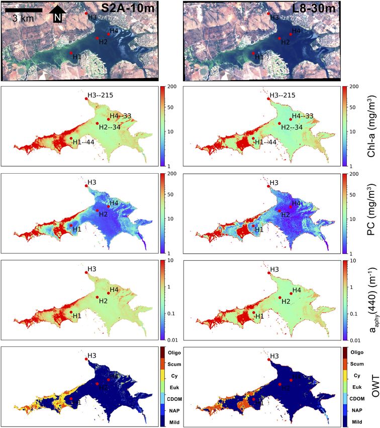
Kravitz et al.                                                                                                         Inland Water Quality Mapping

et al., 2012), which has been attributed to their internal gas             cyanobacteria assemblages, 2) calculations of mixed
vacuoles (Matthews and Bernard, 2013). Due to strong effects               assemblage chl-a fluorescence, 3) modeled PC concentration,
of gas vacuoles on attenuation, rather than absorption, drastic            4) and paired sensor-specific TOA reflectances, which include
differences in water-leaving reflectance occur in mixed                     optically extreme cases and contribution of green vegetation
cyanobacteria assemblages. Thus, vacuolate induced spectral                adjacency. Below, we first describe the parameterization of
scattering (Ganf et al., 1989; Walsby et al., 1995) cannot be              RTM, followed by an examination of typical survived Lw
overlooked when parameterizing RTMs for inland water                       signal at TOA, a description and assessment of state-of-the-art
application. To address these over-simplifications, the                     ML retrieval models, and application to multi-spectral imagery
Equivalent Algal Populations (EAP) model provides an                       with a semi-quantitative validation against in-situ data.
alternative assemblage-based particle modeling approach,
simulating phytoplankton IOPs derived from differences in
cell and assemblage size distributions, dominant pigmentation,             PARAMETERIZATION OF RADIATIVE
cell composition, and ultrastructure (Bernard et al., 2009; Lain           TRANSFER MODEL
et al., 2014).
    While Pahlevan et al. (2020) and Balasubramanian et al.                Aquatic RTM
(2020) present highly convincing results for the transition to             For consistency with natural optical relationships, the IOPs of
ML based models for aquatic particle retrievals using multi-               four datasets were compiled based on the domination of a
spectral sensors, the authors note that adequate atmospheric               particular optical constituent. The EcoLight RTM was then
correction (AC) of top of atmosphere (TOA) radiances to                    used to derive water-leaving reflectances from the IOP builds.
bottom of atmosphere (BOA) reflectances remains one of the                  The first dataset is modeled as typical Case 1 waters where water
largest hurdles to robust, operational space-based water quality           and phytoplankton provide the bulk of the optical signal and
retrievals. Baseline type algorithms, which have proven to be              represent oligotrophic conditions. The bio-optical model in this
robust estimators of trophic status, and relatively insensitive to         dataset closely follows that of Lee (2003), wherein other optical
poor AC, have been utilized on partially corrected bottom-of-              constituents co-vary with phytoplankton biomass. The other
Rayleigh reflectance (BRR) in an attempt to bypass the                      three datasets resemble cyanobacteria dominated inland
requirement for a full AC (Binding et al., 2011; Matthews                  waters, CDOM dominated waters, and inorganic sediment
et al., 2012; Palmer et al., 2015c). This approach is indeed               dominated waters where more complex optical relationships
helpful for smaller water bodies where AC-induced                          persist and optical constituents do not tend to co-vary (Brewin
uncertainty remains very high (Kravitz et al., 2020). Thus, it             et al., 2017). A four-component bio-optical model was used to
follows that ML type models should also perform adequately                 generate the IOPs of these hypothetical inland water cases to be
when utilized on TOA data for inland water pixels. However,                used in the EcoLight RTM (Lee, 2006; Gilerson et al., 2007):
relatively few studies have quantified the actual fraction of the                       a(λ)  aw (λ) + ag (λ) + aphy (λ) + anap (λ)            (1)
isolated water-leaving signal that reaches the satellite sensor over
productive inland water bodies. Utilizing TOA data is                      where aw (λ), ag (λ), aphy (λ), and anap (λ) represent the spectral
theoretically more feasible for turbid waters due to the                   absorptions of water, a combined CDOM/detritus term,
elevated water signal from increased particulate backscattering            phytoplankton, and non-algal particles (NAP), respectively
compared to “darker” oligotrophic waters, which are dominated              (refer to Supplementary Appendix A, Table A1, for a full list
by water absorption. It is quite often cited that of the total             of definitions of symbols and units used throughout this
radiance signal reaching a satellite over water, roughly 10% is            manuscript). Except for the Case 1 dataset, which is defined
due to the upwelling water-leaving radiance (Lw), with                     solely on chlorophyll-a concentration (Cchl) and relationships
atmospheric aerosols and molecular (Rayleigh) scattering                   governing the co-variation of other constituents with Cchl, the
contributing the majority of the signal. However, in a localized           three other datasets are defined by independent values of Cchl, the
modeling study, Martins et al. (2017) found that Lw had the                concentration of nonalgal particles (Cnap), and the absorption of
potential to reach ∼43% of the total signal for red-edge bands of          CDOM at 440 nm (ag(440)). Great care was taken to ensure that
Sentinel-2 MSI over turbid lakes in the Amazon. It is important to         constituent ranges were appropriate and based on natural
understand the extent of the water signal at TOA and its                   populations from the LIMNADES in-situ inland water dataset
sensitivity to certain water and atmospheric parameters in                 (Spyrakos et al., 2018). A table of mode values and standard
order to more thoroughly evaluate models that use TOA data.                deviations used for the lognormal distributions within each
    Here, we aim to explore the potential for developing quick,            dataset can be found in Supplementary Appendix A, Table
robust multi-parameter aquatic retrieval models for both multi-            A3. To generate synthetic datasets representative of natural
spectral and hyper-spectral sensor specifications using a                   waters, values of all constituents were randomly selected from
combined synthetic data and ML approach for productive                     the described lognormal distributions. Derivation and equations
inland waters. Our goal is to begin to simulate the immense                used in modeling components other than phytoplankton are
natural optical variability of inland waters and to address the            common to studies that have parameterized models for Case 2
issues described above. Novel aspects of the synthetic dataset             waters (Bukata, 1995; Twardowski et al., 2001; Gilerson et al.,
presented here include: 1) physics-based, two-layered, size and            2007) and can also be found in Supplementary Appendix A,
type specific phytoplankton IOPs for mixed eukaryotic/                      Table A2.

Frontiers in Environmental Science | www.frontiersin.org               3                                     March 2021 | Volume 9 | Article 587660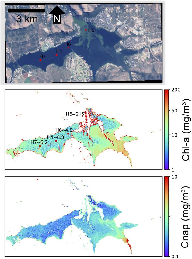
Kravitz et al.                                                                                                             Inland Water Quality Mapping

Phytoplankton Component                                                        where Sf  [0.1,0.2,0.3,0.4,0.5,0.6,0.7,0.8,0.9,1.0], a*cy is the
The total spectral phytoplankton component in Eq. 1 is modeled                 chlorophyll-specific absorption of the cyanobacteria population
as a product of Cchl and the specific chlorophyll absorption                    and a*euk is the chlorophyll-specific absorption for the carotenoid
spectrum.                                                                      containing eukaryotic population. Total scattering and
                                                                               backscattering coefficients of the phytoplankton component
                            aphy (λ)  Cchl p apchl (λ)              (2)
                                                                               (bphy (λ) and bbphy (λ), respectively) are calculated in a similar
where apchl (λ) is the spectral specific chlorophyll absorption                 manner using EAP derived spectral chlorophyll-specific
spectrum in m2/mg. Phytoplankton specific IOPs (SIOPs) for                      scattering and backscattering terms (Supplementary
this work are based on the physics-based two-layered spherical                 Appendix A).
Equivalent Algal Population (EAP) model, where population-                         The admixture weighting factor and input Deff for the
specific refractive indices are used to derive IOPs (Bernard et al.,            eukaryotic population were also randomly varied for the RTM,
2009; Lain and Bernard, 2018). The two-layered spherical                       albeit with some constraints. Several studies have shown that for
geometry consists of a core sphere, acting as the cytoplasm,                   natural populations of oligotrophic to mesotrophic waters, a*euk
and a shell sphere acting as the chloroplast. The EAP model                    tends to decrease with increasing Cchl (Bricaud et al., 1995; Babin
calculates,     from     first    principles,    biophysically-linked           et al., 1996). This rule is not as strict in more complex inland and
phytoplankton absorption and scattering characteristics from                   coastal waters, but rough relationships have been observed
particle refractive indices reflecting the primary light-                       (Matthews and Bernard, 2013). Due to the nature of the EAP
harvesting pigments of various phytoplankton groups (Lain                      model, the magnitudes of the resulting SIOPs are highly
et al., 2014; Lain and Bernard, 2018). IOPs are calculated at                  dependent on the particle size. To generalize this natural
5 nm spectral resolution between 200 and 900 nm and integrated                 relationship in our RTM, input phytoplankton SIOPs of the
over an entire equivalent size distribution represented by effective           carotenoid containing population were constrained by Deff as:
diameters (Deff) between 1 and 50 μm (Bernard et al., 2007; Lain               5 < Deff < 20 μm for 0 < Cchl < 20 mg/m3, 15 < Deff < 35 μm for
et al., 2016). For a hypothetical eukaryotic population, refractive            20 < Cchl < 50 mg/m3, and 30 < Deff < 45 μm for Cchl > 50 mg/m3.
indices are derived from blooms in the Benguela upwelling off                      Ranges for appropriate cyanobacteria admixture weighting
southern Africa, which is typically dominated by chlorophyll-a                 must also be comparable to natural variations as a function of
(chl-a) and the carotenoid pigments, fucoxanthin and peridinin,                phytoplankton biomass. Randomization of weighting factors was
which are the main light harvesting pigments in diatoms and                    constrained based on in-situ phytoplankton abundance and
dinoflagellates, respectively. Because there are minimal                        biomass collected from South African inland waters between
differences within carotenoid pigment refractive indices and                   2016 and 2018 (Kravitz et al., 2020). For a comparison of the
absorption, these two groups were combined into a                              fraction of cyanobacteria abundance as a function of chl-a
generalized set of chl-a—carotenoid IOPs (Bernard et al., 2009;                concentration for both field data and ranges used in the RTM,
Organelli et al., 2017). The EAP model has been consistently                   see Supplementary Figure S1. Given the field data, it was
validated and is considered an accurate phytoplankton model for                assumed that if cyanobacteria are part of the phytoplankton
coastal and inland waters (Evers-King et al., 2014; Mathews and                population, they will tend to dominate at higher biomass
Bernard, 2013; Lain et al., 2016; Smith et al., 2018).                         (i.e., it is rare to find low fractions of cyanobacteria as Cchl
     The EAP two-layered sphere model has also been used to                    rises to extremely hypertrophic levels, if cyanobacteria are
derive IOPs for the optically complex cyanobacteria M.                         present). M. aeruginosa is known to produce extremely high
aeruginosa (Matthews and Bernard, 2013). In this instance, the                 biomass blooms, with the potential to form floating scum mats
core layer is assigned to a highly scattering vacuole, while the shell         that can reach Cchl upwards of 20,000 mg/m3 (Matthews and
layer acts as the chromatoplasm. M. aeruginosa is modeled with a               Bernard, 2013). Extremely hypertrophic cases are reflected in the
Deff of 5 μm for consistency with natural populations. For                     RTM. For Cchl greater than 500 mg/m3, only M. aeruginosa is
derivation of the complex refractive indices, influence of gas                  included as there are no data showing blooms of such an extent
vacuolation, and tuning of the two-layered model for                           for other species.
cyanobacteria, see Matthews and Bernard (2013). IOPs for the
cyanobacteria Aphanizomenon, Anabaena cirinalis and non-                       Chl-a Fluorescence
vacuolate Nodularia spumigena, which were measured in the                      Chl-a fluorescence is potentially an important source of
laboratory, are also included in the dataset (Kutser et al., 2006).            information regarding phytoplankton physiology, size, and/or
The final phytoplankton SIOPs used in the RTM can be found in                   identification (Greene et al., 1992; Behrenfeld et al., 2009),
Supplementary Appendix A, Figure A1.                                           although to what extent remains uncertain. While an integral
     To account for optical variation due to mixed populations, the            component of phytoplankton physiology, fluorescence is often
apchl (λ) term in Eq. 2 is modeled as an admixture of eukaryotic               omitted from RTMs [as in the case of Hieronymi et al. (2017) and
and cyanobacteria SIOPs based on a series of weighting factors.                Fan et al. (2017)] or is modeled as a simplistic Gaussian term
Total apchl (λ) is therefore calculated as the sum of the                      centered at 685 nm with a full width half max (FWHM) of 25 nm
cyanobacteria and eukaryotic populations:                                      (Gilerson et al., 2007; Huot et al., 2007). The magnitude of the
                                                                               depth-integrated radiance contribution by chl-a fluorescence at
                 apchl (λ)  Sf apcy (λ) + 1 − Sf  apeuk (λ)   (3)       685 nm has traditionally been calculated as in Eq. 4 (Huot et al.,

Frontiers in Environmental Science | www.frontiersin.org                   4                                     March 2021 | Volume 9 | Article 587660
Kravitz et al.                                                                                                              Inland Water Quality Mapping

2005; Huot et al., 2007; refer to Supplementary Appendix A for                     While the source of variability of appc (620) in nature is still not
definitions of symbols and units).                                             entirely clear, we can assume that first order variation can result
                                                                              from variable algal/cyanobacteria composition and biomass
     Lf (685)  0.54L−f (685)                                                 effects. Thus, varying appc (620) based on cyanobacteria
                          1∅f p          700
                                              apchl (λ)Eo− (λ)                dominance according to the admixture for each sample is a
                  0.54        Qa [Chl]                       dλ   (4)
                          4πCf           400 K(λ) + KLu (685)                 reasonable approach. Previous studies have generally relied on
                                                                              a fixed appc (620) value for PC estimation models. Considering that
    This modeling approach is an oversimplification for natural                appc (620) has the potential to vary by a factor of 60 in nature (see
coastal and cyanobacteria dominated waters. The approach above                Table 4 in Yacobi et al., 2015), holding it constant is a major
assumes a purely eukaryotic, photosynthetic carotenoid-                       oversimplification, especially for lower Cpc or for cases when
containing phytoplankton assemblage. In other words, it                       cyanobacteria is not the dominant species. In particular, using an
assumes that the modeled population contains all intracellular                invariant appc (620) can result in a dramatic increase in error of PC
chl-a in the fluorescing photosystem II (PSII). Emission spectra of            retrieval when PC:chl-a < 0.5 (Simis et al., 2005; Randolph et al.,
chl-a are a response to photosynthetic pigments that harvest light            2008; Hunter et al., 2010; Li et al., 2015; Yacobi et al., 2015) or
in PSII. However, cyanobacteria generally contain only 10–20%                 when Cpc < 50 mg/m3 (Simis et al., 2005; Ruiz-Verdu et al., 2008;
of their total cellular chl-a in PSII, with no accessory chlorophylls         Yacobi et al., 2015). By employing a model that allows appc (620) to
or carotenoids, and with the remaining cellular chl-a located in              vary based on cyanobacteria dominance, more appropriate values
non-fluorescing photosystem I (PSI) (Johnsen and Sakshaug,                     of appc (620) can be applied to situations of lower PC concentration.
2007; Simis et al., 2012). A second oversimplification pertains                Given the consensus that a PC:chl-a ratio ≥0.5 (mg/m3) implies a
to the shape of the modeled Gaussian fluorescence emission. In                 cyanobacteria dominant water target (Simis et al., 2005; Hunter
reality, while chl-a fluorescence does indeed have a major                     et al., 2010; Yacobi et al., 2015), our admixture of 0–1 was scaled
fluorescence emission around 685 nm, it also has an adjacent                   to a PC:chl-a between 0 and 4, where an admixture of 0.6 (60%
vibrational satellite emission centered around 730–740 nm                     dominance by cyanobacteria in population) is equal to a PC:chl-a
(Govindjee, 2004 and references therein; Lu et al., 2016).                    of 0.5. A strong non-linear relationship was found between PC:
Although generally smaller in amplitude due to increased                      chla-a and appc (620) using in-situ data (Figures 1A,B), and is used
absorption from water farther into the near-infrared (NIR),                   in conjunction with each sample’s scaled admixture parameter to
this 730–740 nm fluorescence emission can potentially                          define a sample specific appc (620) as:
contribute to the water leaving radiance. Supplementary
Appendix B.1 details an updated mathematical derivation for                                       appc (620)  0.0093(Sad )− 0.717                  (6)
the shape and magnitude of the chl-a fluorescence signal
                                                                              where Sad is the scaled admixture parameter. Once both apc (620)
associated with mixed algal populations, which takes into
                                                                              and appc (620) are known, Eq. 5 can be used to calculate a final PC
account differences in PSII physiology for cyanobacteria and
                                                                              concentration.
eukaryotic populations. Equations B1, B2, and B3 were applied
                                                                                   Modeled values for appc (620) using this methodology resulted
to every synthetic spectra to calculate, and add, the modeled chl-a
                                                                              in a mean and median appc (620) of 0.013 ± 0.017 and 0.0041,
fluorescence spectrum.
                                                                              respectively. Simis et al. (2005) used an average value of 0.0095 m2
                                                                              (mg PC)−1 calculated from their in-situ data while Matthews and
Phycocyanin Concentration                                                     Bernard (2013) found the mean appc (620) of various inland water
While the EcoLight radiative transfer code allows Cchl to be                  bodies to range between 0.0072 and 0.0122. Yacobi et al. (2015)
defined as an input to the model, Cpc must be modeled                          found that with Cpc > 10 mg/m3, appc (620) tended to converge on
independently. The calculation of Cpc can be accomplished as                  0.007 m2 (mg PC)−1, but noted that this value is potentially too
follows (Simis et al., 2005):                                                 high. Other studies suggest appc (620) values between 0.004 and
                          Cpc  apc (620)/appc (620)                (5)       0.005 m2 (mg PC)−1 (Li et al., 2015; Mishra et al., 2013; Simis and
                                                                              Kauko, 2012; Jupp et al., 1994). These values are more similar to
where apc (620) is the total absorption due to PC at 620 nm and               our modeled absorption ranges, indicating that our calculated
appc (620) is the specific absorption coefficient of PC at 620 nm.              appc (620) are reasonable (Figure 1). At modeled PC
The apc (620) term must be corrected for the absorption of all                concentrations >50 mg/m3, mean and median appc (620)
other optical constituents and pigments at 620 nm. Most existing              stabilized at 0.0042 ± 0.002 and 0.0034, respectively. The
methods only correct for absorption at 620 nm due to chl-a and                majority of variability in modeled appc (620) occurred at a PC:
not due other accessory pigments; thus, studies suggest that at low           chl-a < 0.5 or a Cpc < 50 mg/m3, consistent with previous findings
PC concentrations (
Kravitz et al.                                                                                                                                   Inland Water Quality Mapping

  FIGURE 1 | (A) appc (620) plotted as a function of PC:chl-a from Matthews and Bernard (2013) and Simis et al. (2005), denoted as M13 and S05, with best fit line in
  black, (B) Visual of admixture scaling, where an admixture of 0.6 (60% dominance by cyanobacteria in population) is equal to a PC:chl-a of 0.5, (C) appc (620) for four
  cyanobacteria groups plotted as a function of PC:chl-a for modeled synthetic data, (D) appc (620) plotted as a function of PC concentration, (E) PC plotted as function of
  chl-a concentration.

at-sensor radiances. The radiance received by an optical sensor                            Mie-generated phase functions and asymmetry parameter, while
can be defined in simple terms following Bulgarelli et al. (2014) as:                       Ext, SSA, and AOT550 were used to tweak the model based on
                                                                                           randomly selected values from the L2 AERONET database. The
                           Ltot  Lpath + LBG + tLu                              (7)
                                                                                           ranges for these parameters are evident in Supplementary Figure
where Ltot is the total radiance received by the sensor, Lpath is the                      S3. For each aquatic Rrs measurement, two random atmospheres
path radiance, which defines the photons scattered into the                                 were modeled, and for each atmosphere, a second identical run
instantaneous field of view (FOV) by the atmosphere alone,                                  was performed with a random contribution of green grass
LBG is the background radiance from neighboring pixels,                                    adjacency between 0.5 and 50%, totaling four atmospheric
which are diffusely scattered into the sensor FOV, Lu is the                               radiative transfer runs per Rrs measurement. Spectral radiance
combined sky reflected and water leaving radiance at the sensor,                            reaching the satellite sensor was calculated as follows:
and t is the diffuse transmittance. LBG is considered as the
radiance introduced due to the adjacency effect (AE), which                                1. The weighted mean of mixed spectral albedo curves was
can lead to large errors in derived products if inter-pixel non-                              computed based on the Adj parameter.
uniformity is very large as in the case for neighboring vegetation,                        2. The atmospheric model was compiled in MODTRAN by tweaking
sand, or snow (Bulgarelli et al., 2017). Optical properties for a                             the standard tropospheric canned model using randomly selected
hypothetical atmospheric column for defining the RTM were                                      parameters (AOT550, SSA, H2O, Ext, Alt, Adj).
compiled from level-2 (L2) derived products from the global                                3. Lu and Lw from Ecolight output were multiplied by atmospheric
Aerosol Robotic Network (AERONET) database (https://aeronet.                                  path transmittance (t) from MODTRAN output to obtain Lu
gsfc.nasa.gov/). The parameters that were directly varied for the                             and Lw at TOA (LuTOA and LwTOA, respectively).
RTM included aerosol optical thickness at 550 nm (AOT550), the                             4. Total radiance at TOA (LtotTOA) was calculated by adding
angstrom extinction coefficient (Ext), single scattering albedo                                LuTOA to the MODTRAN derived atmospheric Lpath, which is
(SSA), the altitude of the hypothetical water target (Alt), water                             the radiance contribution from a scattering atmosphere.
vapor (H2O), and percent adjacency of green grass vegetation                               5. All computations up to this point were performed at full
(Adj). A tropospheric canned model was used to define the initial                              MODTRAN 5 spectral resolution. The sensor specific

Frontiers in Environmental Science | www.frontiersin.org                               6                                             March 2021 | Volume 9 | Article 587660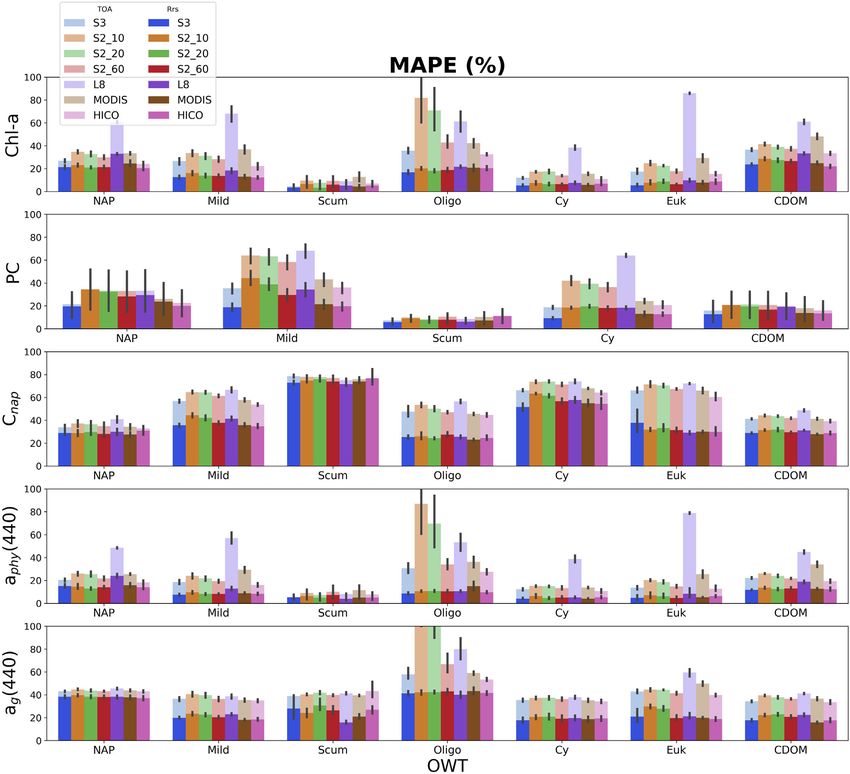
Kravitz et al. Inland Water Quality Mapping
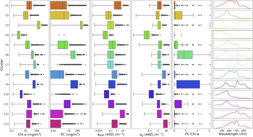
spectral response functions (SRFs) were then applied to curves were defined by band depth, a metric determining the
compute channel radiances. centrality of each curve to the cluster, and are presented in
6. Fraction of surviving Lw reaching the satellite sensor was Figure 2 along with ranges of Cchl, Cpc, anap (440), ag (440),
calculated as LwTOA/LtotTOA. and PC:chl-a. We note that the aim of this paper was not
necessarily to determine the most optimal set of optical water
Radiance at TOA was converted to reflectance using an types (OWTs) for inland waters. Rather, the clustering analysis
analytical derivation as in Hu et al. (2004): was used to demonstrate that RTM can be used to produce OWTs
representative of those observed in nature.
ρt πLpt (F0 cosθ0 ) (8)
The 13 clusters were then condensed into seven manually
where ρt is sensor reflectance at TOA, Lpt is the calibrated at- defined OWTs with ecological relevance. Median Rrs spectra of
sensor radiance after adjustment for ozone and gaseous the seven OWTs are shown in Figure 3, where “Mild” represents
absorption, F0 is the extraterrestrial solar irradiance, and θ0 is low to medium biomass mixed blooms (C2, C5, C11), “NAP”
the solar zenith angle. Adjustment for ozone and molecular represents waters with relatively high non-algal particle loads
species profiles are inherent to the MODTRAN RTM based on (C1, C12), “CDOM” represents waters with relatively high
the specified atmospheric model used (Tropical, Mid-Latitude CDOM absorption (C8, C13), “Euk” represents eukaryotic
Summer, or Mid-Latitude Winter). algal blooms (C7), “Cy” represents cyanobacteria blooms (C6,
C9), “Scum” represents Microcystis floating scum conditions
(C3), and “Oligo” represents oligotrophic to slightly
DATA PREPARATION AND TRAINING mesotrophic waters (C4, C10). The resulting median Rrs
spectra from each manually defined OWT are shown in
Data Smoothing and Clustering Figure 4 and match exceptionally well with in-situ water types
Roughly 70,000 Rrs spectra were modeled with coincident Cchl, in Kravitz et al. (2020; their Figure 4) for productive South
Cpc, Cnap, and associated IOPs. A clustering procedure was African waters.
undertaken to identify distinct optical clusters with respect to
reflectance within the dataset. Clustering of water types on the Machine Learning Models
basis of optical properties has been commonly employed since the K-Nearest Neighbors
1970s as a method to direct the application of Earth observation The K-nearest neighbor (KNN) algorithm (Altman, 1992) is a
(EO) for aquatic purposes (Moore et al., 2001; Moore et al., 2009; non-parametric, lazy learning model, that can be used for
Moore et al., 2014; Vantrepotte et al., 2012; Spyrakos et al., 2018). regression (KNR) and classification (KNC). The model is
Clustering of optical data has historically been beneficial for “lazy” in that all training data are used in the testing phase.
demonstrating underlying bio-optical relationships and This allows for faster training times, but slower and costlier
variability, and guiding the development and application of testing and prediction. The core of the KNN model is based
retrieval models. For consistency with previous clustering on identifying similarity between datapoints, which is done by
applications in coastal and inland waters, the functional data calculating distance or proximity of all points to each other, and
analysis (FDA) approach of Spyrakos et al. (2018) was closely assuming similar datapoints are close to each other. The model is
followed, although only briefly discussed here. A full analysis of tuned by choosing the optimal number for K, which defines the
historical clustering techniques is beyond the scope of this paper, number of training samples closest in distance to the new point,
and readers are directed to Spyrakos et al. (2018 and references followed by a value prediction. How distance between points is
therein) for a more comprehensive overview of clustering calculated can also be defined. KNN has become popular for its
approaches. A comprehensive guide to FDA can also be found simplicity and fast training with minimal tuning; however,
in Ramsay and Silverman (2006). predictions take much longer with increasing training data or
Prior to clustering, all Rrs spectra were normalized by their number of features.
respective integrals, as a way to standardize amplitude variation
attributed to concentrations of optically active constituents. Each Random Forest
spectrum was deconvolved into 26 cubic basis functions, of which The random forest (RF) algorithm (Ho, 1998; Breiman, 2001) is
a linear combination results in a smoothed Rrs spectra an extension of the decision tree model, which, in simple terms,
(Supplementary Figure S4). The same B-spline representation constructs a series of yes/no questions about the data until an
was used here as in Spyrakos et al. (2018), with the inclusion of answer is reached and can be used for classification (RFC) or
one extra knot in the 800–900 nm region. The actual clustering by regression (RFR). RF is an ensemble method that builds tens to
k-means was then performed on the 26 basis coefficients from the thousands of decision trees based on random sampling of training
cubic functions. This acts as a method of dimensional reduction subsets and features, and averages (or majority voting for
that removes excessive local variability, keeps independence classification) all the results for a final product. There are a
among variables, and allows for a customizable smoothing number of tunable hyperparameters that generally differ in
approach through number and placement of knots. k-means how the questions are formed and define the depth of the
was used to cluster the dataset of basis coefficients into 13 trees. Training can be computationally expensive with
distinct clusters. Information on how the number of clusters extremely large datasets; however, prediction is much faster
was chosen can be found in Supplementary Material. Median than can be achieved using KNN.
Frontiers in Environmental Science | www.frontiersin.org 7 March 2021 | Volume 9 | Article 587660
Kravitz et al.                                                                                                                               Inland Water Quality Mapping

  FIGURE 2 | Ranges of Cchl, Cpc, anap (440), ag (440), and PC:chl-a for each defined synthetic cluster along with median Rrs spectra. Additional IOP ranges can be
  found in Supplementary Material.

  FIGURE 3 | Median Rrs spectra of the seven manually defined OWTs derived from the set of 13 clusters. The inset shows the same spectra on a standardized scale,
  achieved by removing the mean and scaling to unit variance in order to better show shape variation.

XGBoost                                                                                  (boosting), until no further model improvements can be made.
The extreme gradient boosting (XGBoost) framework (Chen and                              Gradient boosting then uses the gradient descent algorithm to
Guestrin, 2016) advances the RF model by including gradient                              minimize the loss when adding new models. XGBoost runs
boosted decision trees. This ensemble method builds new, weak                            exceptionally well on tabulated data for classification or
models sequentially by minimizing errors from previous models                            regression purposes and has dominated data science
and increasing the influence of higher performing models                                  competitions in recent years due to its efficiency and power.

Frontiers in Environmental Science | www.frontiersin.org                             8                                            March 2021 | Volume 9 | Article 587660
Kravitz et al.                                                                                                                       Inland Water Quality Mapping

  FIGURE 4 | A technical flowchart showing the summarized data development and training stages of ML algorithms to retrieve water quality products (“WQ
  Products”). Sx indicates one of the seven band configurations used in data preparation. K represents the specific iteration of k-fold cross validation.

Multi-Layer Perceptron                                                              six multispectral and hyperspectral sensor specifications: Sentinel 3
The multi-layer perceptron (MLP) is a type of classical artificial                   Ocean and Land Colour Imager (S3-OLCI), Sentinel 2 multi-
neural network (ANN) that is capable of learning any non-linear                     spectral imager (S2-MSI) at the sensor’s 60, 20, and 10 m band
mapping function and can be thought of as a universal                               configurations, Landsat 8 operational land imager (L8-OLI),
approximation algorithm. The fundamental units of MLPs are                          the moderate resolution imaging spectroradiometer (MODIS),
artificial neurons, each with their own weighting and activation                     and a hypothetical hyperspectral configuration based on the
functions. The activation function maps the summed weighted                         hyperspectral imager for the coastal ocean (HICO). As a means
inputs to the output of the neuron. Individual neurons can be                       of dimensionality reduction, the seventh configuration consisted of
merged into networks of neurons, generally in the form of a                         the scores from the first ten EOF modes from a singular value
visible input layer and subsequent hidden layers, including the                     decomposition (SVD) of the entire dataset for HICO bands. In this
output layer. The activation function of the output layer                           instance, the ten scores were used as input to the ML model,
constrains the model for the specific type of problem                                replacing the channel reflectances. See Table 1 for a list of all sensor
(i.e., regression or classification). With increasing                                band configurations.
computational resources, deep multi-layer networks composed                             Inputs to each model consist of three sets of features: 1) the
of multiple layers of hundreds of neurons can now be constructed                    visible and near infrared (NIR) bands of the specific sensor
for highly complex problems.                                                        configuration, 2) the Sun and sensor geometry if the model is
                                                                                    applied to TOA reflectance, and 3) a selection of feature
Cross Validation                                                                    interactions, which include band ratios and spectral derivative
Model Inputs and Outputs                                                            type indices (Table 1). Feature tuning and extraction can have
The primary input to each ML algorithm is the visible and near                      dramatic effects on resulting model errors or accuracies.
infrared channel TOA reflectances or Rrs of the specific sensor and                   Generally, interactions among variables can supplement the
band configuration. The modeled synthetic data were resolved to                      individual predictor variables to enhance the feature space to

Frontiers in Environmental Science | www.frontiersin.org                        9                                         March 2021 | Volume 9 | Article 587660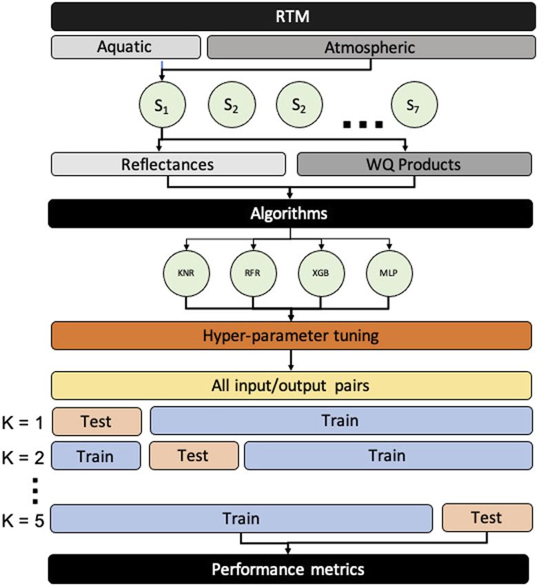
Kravitz et al. Inland Water Quality Mapping
TABLE 1 | Inputs for ML models. Inputs are the same for the four ML models used in this study, except for Sun and sensor geometries, which were only used on TOA
models. References from 1 to 13 (Gower et al., 2008; Hu, 2009; Dall’Olmo and Gitelson, 2005; Mishra and Mishra, 2012; Gower et al., 1999; Moses et al., 2009; Qi et al.,
2014; Matthews et al., 2012; Hunter et al., 2010; Mishra et al., 2013; Liu et al., 2017; Dekker, 1993; Shi et al., 2015):
Sensor Bands Geometries Feature interactions
L8-OLI B1, B2, B3, B4, B5 OZA, OAA, B4/B3, B4/B2, B4/B1, B3/B2, B3/B1, B2/B1
S2- B2, B3, B4, B8 SZA, SAA B4/B3, B4/B2, B3/B2
MSI 10 m
S2- B2, B3, B4, B5, B6, B7, B8, B8A B5/B4, B5/B3, B5/B2, B4/B3, B4/B2, B3/B2, MCI1, FAI2,
MSI 20 m D3b3, NDCI4
S2- B1, B2, B3, B4, B5, B6, B7, B8, B8A B5/B4, B5/B3, B5/B2, B4/B3, B4/B2, B3/B2, MCI, FAI, D3b,
MSI 60 m NDCI
S3-OLCI Oa1, Oa2, Oa3, Oa4, Oa5, Oa6, Oa7, Oa8, Oa9, Oa10, Oa11, Oa12, FLH5, MCI, FAI, M2b6, D3B, NDCI, PCI7, SIPF8, H103b9,
Oa16, Oa17, Oa18 M133b10, L4b11, D9312
MODIS B1, B2, B3, B4, B8, B9, B10, B11, B12, B13, B14, B15, B16 FLH, SIPF, FAI, Shi1513
HICO All bands 400–900 nm None
HICO-SVD EOF modes 1–10 None
improve the predictive capability of the models. This has been the Supplementary Material. A technical roadmap of the data
confirmed for aquatic cases (Ruescas et al., 2018; Hafeez et al., development and training stages is shown in Figure 4. All the
2019) where including band interactions such as band ratios or analyses were performed using a personal laptop equipped with
line height models has improved model performance. Model 16 GB of RAM.
outputs are concentrations of chl-a, PC, and NAP in mg/m3, as
well as aphy in m−1, and the OWT.
The Rrs dataset contains roughly 70,000 samples, while the RESULTS
TOA reflectance dataset contains roughly 260,000 samples. For
each dataset, models were evaluated using k-fold cross validation Surviving Lw at TOA
where the data were split into 80% for training and 20% for The average percent contributions of the surviving water signal at
testing for five folds in order to avoid sampling bias (Figure 4). Ltot for the seven manually defined OWTs derived above for
Performance metrics used in the evaluation consist of both linear specific visible and NIR bands are shown in Figure 5. The high
and log-transformed root mean squared error (RMSE and inter- and intra-variability of the percent contribution of the Lw
RMSELE, respectively), relative RMSE (rRMSE), bias, and signal is evident. Relatively low contribution from the 443 nm
median absolute percent error (MAPE). band is common amongst OWTs. This region encompasses high
amounts of absorption amongst the different aquatic optical
Hyper-Parameter Tuning constituents as well as significant interference from
To obtain results of the highest fidelity possible, ML models atmospheric molecular Rayleigh scattering. Consequently, this
require optimization of their respective hyper-parameters band only reaches above 20% contribution in extremely scattering
before training of the actual ML model for product retrieval. conditions containing relatively low amounts of blue absorption
The hyper-parameters govern the training process itself and due to decreased phytoplankton and CDOM. There is a general
define the model architecture. These parameters are not increase in surviving aquatic signal with increased inorganic
updated during the learning process and are used to sediment, as well as with a more dominant phytoplankton
configure the model in various ways. In this study, hyper- component. The fraction of Lw at TOA is also relatively
parameter tuning was accomplished using a grid search, elevated in OWTs comprising greater concentrations of PC,
which builds a model for each possible combination of all particularly the red edge band. When cyanobacteria dominate,
hyper-parameters provided, evaluates each model, and selects Lw at TOA fractions have the potential to reach 40% for red/NIR
the architecture with the lowest mean squared error (MSE) for bands with chl-a concentrations as low as 10 mg/m3, while
regression models, or accuracy for classification models. The maxing out at an average of roughly 60% for the 709 nm band
best performing combination of hyper-parameters is then just above 100 mg/m3 (data not shown). When eukaryotic algae
applied to train the ML model using the entire dataset. dominate, average surviving Lw at TOA fraction only exceeds 20%
Computational requirements for extensive hyper-parameter for the NIR bands and at highly elevated chl-a concentrations.
tuning can be very high, especially when dealing with more This relationship is also apparent when comparing subdued Lw at
complex or deep models. The models used here were trained TOA fractions of the eukaryotic bloom OWT (“Euk”), which
with minimal hyper-parameter tuning, as conducting an represents high biomass eukaryotic algae blooms, vs. the “Cy”
exhaustive grid search exercise for every trained model OWT dominated by cyanobacteria and containing much higher
explored in this study would be very computationally PC:chl-a ratios (Figure 6). OWTs consisting of relatively high
expensive. However, a brief hyper-parameter tuning exercise mineral concentrations (“NAP” OWT) yield broadly elevated
was performed to optimize each of the models’ most sensitive surviving Lw at TOA, with fractions ranging from 20 to 60% for
hyperparameters. Final model hyper-parameters are listed in the green to NIR bands.
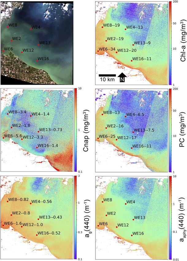
Frontiers in Environmental Science | www.frontiersin.org 10 March 2021 | Volume 9 | Article 587660Kravitz et al. Inland Water Quality Mapping FIGURE 5 | Fraction of surviving Lw at Ltot for specific wavelengths for each derived OWT. Model Performance Against Synthetic at TOA, such as the Oligo or Euk water types, experience the Dataset greatest difference in product retrieval error when comparing Evaluation of overall model performance applied to TOA retrievals at Rrs or TOA. When comparing sensor configurations, reflectance or Rrs spectral data, per sensor, can be found in L8-OLI generally observes the largest discrepancies between Supplementary Appendix C for retrieval of chl-a, PC, and product retrievals at Rrs and TOA, most significantly for NAP concentrations, and aphy(440). The MLP overwhelmingly pigment retrievals and aphy (440). That said, L8 produces outperforms the other ML models in almost every case in terms of smaller errors at TOA in oligotrophic to mesotrophic waters MAPE and RMSELE when evaluated against the entire dataset (Oligo OWT) when compared to the S2-MSI 10 m and 20 m band using Rrs data. A lower MAPE/RMSELE would signify better configurations. Other than for the Oligo OWT, the difference in performance (Supplementary Appendix Figure C1). When error between ag(440) retrievals at Rrs and TOA are relatively applied to TOA reflectance, MLP still generally performs the consistent between sensor configurations. best, although with exceptions in specific cases. The KNR model generally performs the worst for retrievals when applied to both Case Study Application Rrs and TOA reflectance. Considering the variability of these Hartbeespoort Dam, South Africa products within the synthetic dataset, the MLP shows promising To assess the spatial integrity of retrieval products as well as test predictive capabilities for all trophic states. cross-sensor consistency, a semi-quantitative examination of Figure 6 shows the MAPE of the MLP algorithm retrievals by productive freshwater scenes was undertaken. Figure 7 shows OWT for each sensor using both Rrs and TOA reflectance data. the results of MLP products retrievals using S2-MSI in the 10 m Significant differences can be observed in the capability of the band configuration and L8 TOA reflectances (refer to Table 1 MLP algorithm for chl-a, PC, and NAP concentration retrievals, for band configurations). The scene focuses on Hartbeespoort as well as retrievals for absorption at 440 nm by phytoplankton Dam, South Africa, on October 27, 2016. Hartbeespoort Dam is and CDOM, due to the different band configurations. The OWT a small, optically complex reservoir that experiences frequent can also significantly affect retrieval performance differently cyanobacteria and floating aquatic macrophyte blooms. The among sensors. When using Rrs data, product retrievals by dam is traditionally a very difficult remote sensing target due sensor do not show much intra-variability within OWTs, and to its small size and the optically complex nature of the water. on average, yield errors ranging from 20 to 40% amongst OWTs. While both sensor configurations have similar, limited spectral Exceptions to this include errors >50% for Cnap retrieval, and resolution, L8-OLI provides the advantage of an additional
Kravitz et al.                                                                                                                                 Inland Water Quality Mapping

  FIGURE 6 | Median absolute percent error (MAPE) for MLP derived products (from top-to-bottom: chl-a, PC, and NAP concentrations, absorption of
  phytoplankton, and ag at 440 nm). Retrieval errors using Rrs are in solid bright colors, while retrieval errors using TOA reflectance are stacked in corresponding opaque
  colors. Lower MAPE corresponds to better performance. Error bars represent the standard deviation for the five-fold cross validation.

is apparent. L8 slightly underestimates chl-a outside of the intense                      to cyanobacteria dominated conditions, to milder sub-surface
bloom in the western part of the dam relative to the S2 retrieval.                        blooms in the Eastern basin. This can also be visualized in the
The PC and aphy(440) retrievals, although not validated with in-                          RGB as fading of the intensity of the green color, where the
situ data, depict realistic relationships and ranges associated with                      absorption of the water becomes stronger due to less
the chl-a product. Strong consistency between the two sensors is                          phytoplankton biomass. S2 appears to differentiate scum and
also evident. Inter-comparison of products also depicts the de-                           high cyanobacteria concentrations more effectively than L8. This
coupling of PC and chl-a estimation, as evidenced by strong                               is potentially the result of a combination between the inclusion of
spatial consistency between chl-a and aphy(440), while PC is more                         the red-edge band utilized for S2, as well as smaller pixel size. AC
drastically concentrated in the Western basin, and substantially                          over intense bloom waters such as these are error prone and can
lower in the Eastern basin. The scene demonstrates the capability                         lead to large uncertainties in retrieval products (Kravitz et al.,
for extremely dynamic ranges of water quality product retreivals.                         2020). As the AC and product retrieval are essentially performed
Water type classification using the two configurations is also                              together in the inversion, the strong water-leaving signal at TOA
remarkably consistent. Depicting a gradient of scum conditions,                           allows for very reasonable product retrieval estimates.

Frontiers in Environmental Science | www.frontiersin.org                             12                                             March 2021 | Volume 9 | Article 587660
Kravitz et al.                                                                                                                                    Inland Water Quality Mapping

  FIGURE 7 | MLP product retrievals over Hartbeespoort Dam on October 27, 2016. The left column shows retrievals using S2 10 m configuration while the right
  column is the L8 retrievals. All products are derived from TOA reflectance. On the chl-a panels, in-situ sampling points (red dots) are labeled with the station name
  followed by the measured quantity of chl-a, in units of mg/m3 (e.g., H1--44 indicates station H1 with a measured in-situ chl-a concentration of 44 mg/m3). In-situ data are
  from Kravitz et al. (2020).

   Figure 8 displays another instance of same-day chl-a retrievals                          can be visualized in the RGB image and is consequently flagged
at Hartbeespoort Dam on March 29, 2017. A large water hyacinth                              out in product retrievals. This poses a very difficult scenario for
bloom had begun spreading from the North-Eastern basin which                                medium resolution sensors, with potential for strong signal

Frontiers in Environmental Science | www.frontiersin.org                               13                                             March 2021 | Volume 9 | Article 587660
Kravitz et al.                                                                                                                   Inland Water Quality Mapping

                                                                                      of multi-parameter inversion using only four bands in the 10 m
                                                                                      configuration (Figure 10), while the 60 m configuration uses nine
                                                                                      bands in the vis/NIR (Figure 9). Despite the five spectral band
                                                                                      difference, product consistency is very strong and respectably
                                                                                      correlated with in-situ measurements. The higher spatial
                                                                                      resolution in the 10 m configuration also demonstrates the de-
                                                                                      coupling of water quality products for a slick of disturbed water
                                                                                      emanating from the lower western basin. The high spatial
                                                                                      resolution captures the elevated dissolved organic and non-
                                                                                      algal content in the disturbed water.
                                                                                          A short time-series analysis was conducted at station WE4 of
                                                                                      Lake Erie during the bloom period of 2018 between June and
                                                                                      October. In-situ field data are plotted along with product
                                                                                      retrievals for S3, S2 in both 10 m and 60 m configurations,
                                                                                      and L8, all using TOA reflectance data (Figure 11). All non-
                                                                                      cloudy images available for each sensor during the time period
                                                                                      were downloaded from either the United States Geological Survey
                                                                                      (USGS) Earth Explorer (https://earthexplorer.usgs.gov/), or the
                                                                                      European Space Agency (ESA) Copernicus Open Access Hub
                                                                                      (https://scihub.copernicus.eu/). Considering the highly dynamic
                                                                                      nature of bloom and water dynamics in the western basin, the
                                                                                      multi-spectral sensors were able to adequately track the progress
                                                                                      of two subsequent cyanobacteria blooms during the time period.
                                                                                      Other than some outlying instances of apparent model failure
                                                                                      using S3, which would inquire further inspection, Figure 11
                                                                                      demonstrates the capability of a multi-sensor approach to fill
                                                                                      temporal gaps due to clouds and revisit times.
                                                                                          Figure 12 displays the results of MLP product retrievals using
                                                                                      L8-OLI and S2-MSI plotted against same-day in-situ field data for
                                                                                      three images of South African waters, which only include chl-a
  FIGURE 8 | MLP product retrievals over Hartbeespoort Dam on March
  29, 2017 using L8 TOA reflectance data. For the chl-a panel, in-situ sampling        validation, and two images of Lake Erie, which also include PC,
  points (red dots) are labeled with the station name followed by the measured        ag(440), and Cnap, for a total of 72 chl-a matchups and 46
  quantity of chl-a, in units of mg/m3. In-situ data are from Kravitz et al.          matchups for each of PC, ag(440), and Cnap, totaling 216 total
  (2020).                                                                             point matchups. Although it is not conventional to aggregate
                                                                                      multiple sensors and their associated products, the figure
                                                                                      provides an estimation of total error, as calculated using the
contamination for less productive water pixels from adjacent                          MAPE, for the three sensor configurations on a limited number of
bright vegetation pixels. Chl-a product retrieval estimates                           validation points. A combined MAPE of 52% was achieved for the
correlate very well with in-situ measurements, even adjacent to                       four products at three multi-spectral sensor configurations using
the water hyacinth. Product estimations of Cnap, although not                         TOA reflectance. The error adequately corresponds to results
validated with in-situ data, show a realistic de-coupling of organic                  achieved using synthetic data in Figure 6 for these water types, as
and inorganic material, with high NAP concentrations displayed                        well as results from other studies using ML trained on in-situ data
in the sediment-laden South Eastern arm of the dam.                                   (Balasubramanian et al., 2020; Pahlevan et al., 2020).

Lake Erie, United States
A separate semi-quantitative validation of MLP retrieval products                     DISCUSSION
was conducted for the western basin of Lake Erie, USA. Figures
9,10 show product retrievals during a mild cyanobacteria bloom                        Machine Learning Models
on August 13, 2018 using S2 TOA reflectances in the 60 m and                           Four out-of-the-box ML models were trained using synthetic data
10 m band configurations, respectively. Retrieval products are                         and applied to EO data using the Python programming language.
qualitatively validated with in-situ measurements of chl-a, PC,                       We note that the aim of this study was not to produce an optimal,
Cnap, and ag(440) collected and distributed by the National                           finalized retrieval model for operational use, but rather to explore
Oceanographic and Atmospheric Administration (NOAA)                                   the capacity of a range of well documented ML models to make
Great Lakes Environmental Research Laboratory (GERL) and                              adequate predictions of water quality variables, trained from
National Centers for Environmental Information (NCEI)                                 synthetic optical and radiometric data. ML has proven an
(https://www.glerl.noaa.gov/res/HABs_and_Hypoxia/habsMon.                             extremely powerful tool that is now more accessible and easier
html). Comparison of the two figures demonstrates the capability                       to implement than ever before. This study confirms other reports

Frontiers in Environmental Science | www.frontiersin.org                         14                                    March 2021 | Volume 9 | Article 587660
You can also read