Think Globally, Fit Locally: Unsupervised Learning of Low Dimensional Manifolds
←
→
Page content transcription
If your browser does not render page correctly, please read the page content below
Journal of Machine Learning Research 4 (2003) 119-155                                Submitted 6/02; Published 6/03

                          Think Globally, Fit Locally:
              Unsupervised Learning of Low Dimensional Manifolds

Lawrence K. Saul                                                                     LSAUL @ CIS . UPENN . EDU
Department of Computer and Information Science
University of Pennsylvania
200 South 33rd Street
557 Moore School - GRW
Philadelphia, PA 19104-6389, USA
Sam T. Roweis                                                                    ROWEIS @ CS . TORONTO . EDU
Department of Computer Science
University of Toronto
6 King’s College Road
Pratt Building 283
Toronto, Ontario M5S 3G4, CANADA

Editor: Yoram Singer

                                                        Abstract
     The problem of dimensionality reduction arises in many fields of information processing, including
     machine learning, data compression, scientific visualization, pattern recognition, and neural com-
     putation. Here we describe locally linear embedding (LLE), an unsupervised learning algorithm
     that computes low dimensional, neighborhood preserving embeddings of high dimensional data.
     The data, assumed to be sampled from an underlying manifold, are mapped into a single global
     coordinate system of lower dimensionality. The mapping is derived from the symmetries of locally
     linear reconstructions, and the actual computation of the embedding reduces to a sparse eigen-
     value problem. Notably, the optimizations in LLE—though capable of generating highly nonlinear
     embeddings—are simple to implement, and they do not involve local minima. In this paper, we de-
     scribe the implementation of the algorithm in detail and discuss several extensions that enhance its
     performance. We present results of the algorithm applied to data sampled from known manifolds,
     as well as to collections of images of faces, lips, and handwritten digits. These examples are used to
     provide extensive illustrations of the algorithm’s performance—both successes and failures—and
     to relate the algorithm to previous and ongoing work in nonlinear dimensionality reduction.

1. Introduction

Many problems in machine learning begin with the preprocessing of raw multidimensional sig-
nals, such as images of faces or spectrograms of speech. The goal of preprocessing is to obtain
more useful representations of the information in these signals for subsequent operations such as
classification, denoising, interpolation, visualization, or outlier detection. In the absence of prior
knowledge, such representations must be learned or discovered automatically. Automatic methods
which discover hidden structure from the statistical regularities of large data sets can be studied in
the general framework of unsupervised learning (Hinton and Sejnowski, 1999).

c 2003 Lawrence K. Saul and Sam T. Roweis.
S AUL AND ROWEIS
Two main goals have been proposed for algorithms in unsupervised learning: density estima-
tion and dimensionality reduction. The goal of density estimation is to learn the parameters of a
probabilistic model that can be used to predict or assess the novelty of future observations. The
goal of dimensionality reduction is to obtain more compact representations of the original data that
capture the information necessary for higher-level decision making. A recent trend in machine
learning has been to pursue these goals simultaneously, with probabilistic generative models of raw
sensory inputs whose hidden variables represent low dimensional degrees of freedom (Attias, 1999;
Dayan et al., 1995; Hyvärinen, 1998; Roweis, 1998; Roweis et al., 2002; Tipping and Bishop, 1999).
However, the goal of dimensionality reduction can also be pursued in a non-probabilistic and non-
parametric setting. This is the approach taken here, leading to an efficient eigenvector method for
nonlinear dimensionality reduction of large data sets.
Our work addresses a longstanding problem at the intersection of geometry and statistics: to
compute a low dimensional embedding of high dimensional data sampled (with noise) from an
underlying manifold. Many types of high dimensional data can be characterized in this way—
for example, images generated by different views of the same three dimensional object. Beyond
applications in machine learning and pattern recognition, the use of low dimensional manifolds to
represent continuous percepts is also a recurring theme in computational neuroscience (Seung and
Lee, 2000). The goal of our algorithm is to learn such representations from examples: to discover—
in a general setting, without the use of a priori knowledge—the few degrees of freedom that underlie
observed modes of continuous variability.
Two canonical forms of dimensionality reduction are the eigenvector methods of principal com-
ponent analysis (PCA) (Jolliffe, 1986) and multidimensional scaling (MDS) (Cox and Cox, 1994).
Most applications of PCA and MDS involve the modeling of linear variabilities in multidimensional
data. In PCA, one computes the linear projections of greatest variance from the top eigenvectors of
the data covariance matrix. In MDS, one computes the low dimensional embedding that best pre-
serves pairwise distances between data points. If these distances correspond to Euclidean distances
— the case of so-called classical scaling — then the results of MDS are equivalent to PCA (up to
a linear transformation). Both methods are simple to implement, and their optimizations are well
understood and not prone to local minima. These virtues account for the widespread use of PCA
and MDS, despite their inherent limitations as linear methods.
Recently, we introduced a more powerful eigenvector method—called locally linear embedding
(LLE)—for the problem of nonlinear dimensionality reduction (Roweis and Saul, 2000). This prob-
lem is illustrated by the manifolds in Figure 1. In these examples, dimensionality reduction by LLE
succeeds in recovering the underlying manifolds, whereas linear embeddings by PCA or MDS map
faraway data points to nearby points in the plane, creating distortions in both the local and global
geometry. Like PCA and MDS, our algorithm is simple to implement, and its optimizations do not
involve local minima. Unlike these methods, however, it is capable of generating highly nonlinear
embeddings, and its main optimization involves a sparse eigenvalue problem that scales well to
large, high dimensional data sets.
Note that mixture models for local dimensionality reduction (Fukunaga and Olsen, 1971;
Ghahramani and Hinton, 1996; Kambhatla and Leen, 1997), which cluster the data and perform
PCA within each cluster, do not address the problem considered here—namely, how to map high
dimensional data into a single global coordinate system of lower dimensionality. In particular, while
such models can be used to discover clusters in high dimensional data and to model their density,
120U NSUPERVISED LEARNING OF LOW DIMENSIONAL MANIFOLDS
(A) (B) (C)
Figure 1: The problem of nonlinear dimensionality reduction, as illustrated for three dimensional
data (B) sampled from two dimensional manifolds (A). An unsupervised learning al-
gorithm must discover the global internal coordinates of the manifold without external
signals that suggest how the data should be embedded in two dimensions. The LLE algo-
rithm described in this paper discovers the neighborhood-preserving mappings shown in
(C); the color coding reveals how the data is embedded in two dimensions.
121S AUL AND ROWEIS
they could not be used to compute the two dimensional embeddings in the rightmost panels of
Figure 1.
In this paper, we describe the LLE algorithm, providing significantly more examples and de-
tails of its implementation than can be found in our earlier work (Roweis and Saul, 2000). We
also discuss a number of extensions that enhance its performance. The organization of this paper
is as follows: In Section 2, we describe the algorithm in general terms, focusing on its main proce-
dures and geometric intuitions. In Section 3, we illustrate the algorithm’s performance on several
problems of different size and dimensionality. In Section 4, we discuss the most efficient ways to
implement the algorithm and provide further details on the nearest neighbor search, least squares
optimization, and eigenvalue problem. In Sections 5 and 6, we describe a number of extensions
to LLE, including how to estimate and/or enforce the dimensionality of discovered manifolds, as
well as how to derive mappings that generalize the results of LLE to examples outside the train-
ing set. Finally, in Section 7, we compare LLE to other eigenvector-based methods for clustering
and nonlinear dimensionality reduction (Belkin and Niyogi, 2002; Ng et al., 2002; Schölkopf et al.,
1998; Shi and Malik, 2000; Tenenbaum et al., 2000; Weiss, 1999) and mention several directions
for future work.
2. Algorithm
The LLE algorithm, summarized in Figure 2, is based on simple geometric intuitions. Essentially,
the algorithm attempts to compute a low dimensional embedding with the property that nearby
points in the high dimensional space remain nearby and similarly co-located with respect to one
another in the low dimensional space. Put another way, the embedding is optimized to preserve the
local configurations of nearest neighbors. As we shall see, under suitable conditions, it is possible
to derive such an embedding solely from the geometric properties of nearest neighbors in the high
dimensional space. Indeed, the LLE algorithm operates entirely without recourse to measures of
distance or relation between faraway data points.
To begin, suppose the data consist of N real-valued vectors ~Xi (or inputs), each of dimensional-
ity D, sampled from a smooth underlying manifold. Provided there is sufficient data (such that the
manifold is well-sampled), we expect each data point and its neighbors to lie on or close to a locally
linear patch of the manifold. More precisely, by “smooth” and “well-sampled” we mean that for
data sampled from a d-dimensional manifold, the curvature and sampling density are such that each
data point has on the order of 2d neighbors which define a roughly linear patch on the manifold
with respect to some metric in the input space. Under such conditions, we can characterize the local
geometry in the neighborhood of each data point by linear coefficients that reconstruct the data point
from its neighbors. The LLE algorithm derives its name from the nature of these reconstructions: it
is local, in the sense that only neighbors contribute to each reconstruction, and linear, in the sense
that reconstructions are confined to linear subspaces.
In the simplest formulation of LLE, one identifies K nearest neighbors per data point, as mea-
sured by Euclidean distance. (More sophisticated neighborhood criteria are discussed in Section 4.)
Reconstruction errors are then measured by the cost function:
2
E (W ) = ∑ ~Xi − ∑ jWi j ~X j , (1)
i
122U NSUPERVISED LEARNING OF LOW DIMENSIONAL MANIFOLDS
LLE ALGORITHM 1 Select neighbors.
1. Compute the neighbors of
each data point, ~Xi .
Xi
2. Compute the weights Wi j
that best reconstruct each
data point ~Xi from its neigh-
2 Xi Wik Xk
Reconstruct
bors, minimizing the cost in with linear
Wij
weights. Xj
Equation (1) by constrained
linear fits.
3. Compute the vectors ~Yi
best reconstructed by the
Yi Wik Yk
weights Wi j , minimizing
the quadratic form in Wij Yj
Equation (2) by its bottom
nonzero eigenvectors. 3 Map to embedded coordinates.
Figure 2: Summary of the LLE algorithm, mapping high dimensional inputs ~Xi to low dimensional
outputs ~Yi via local linear reconstruction weights Wi j .
Xi Xj
Σ Wij X j
j
Xj’
Figure 3: A data point ~Xi , its neighbors ~X j , and its locally linear reconstruction ∑ j Wi j ~X j . The
reconstruction weights are constrained to satisfy ∑ j Wi j = 1.
which adds up the squared distances between all the data points and their reconstructions. The
weight Wi j summarizes the contribution of the jth data point to the ith reconstruction. To compute
the weights, we minimize the cost function in Equation (1) subject to two constraints: a sparseness
constraint and an invariance constraint. The sparseness constraint is that each data point ~Xi is
reconstructed only from its neighbors, enforcing Wi j = 0 if ~X j does not belong to this set. The
invariance constraint is that the rows of the weight matrix sum to one: ∑ j Wi j = 1. The reason for
this latter constraint will become clear shortly. The optimal weights Wi j subject to these constraints
are found by solving a set of constrained least squares problems, as discussed further in Section 4.
123S AUL AND ROWEIS
0.5 0.4 0
0.5 0.6 1
Figure 4: The effects of shearing on reconstruction weights. Shown are the optimal weights that
linearly reconstruct the black point in terms of its gray neighbors; the resulting recon-
structions are indicated by white squares. Note that the optimal weights and linear recon-
structions are not invariant to shear transformations.
Note that the constrained weights that minimize these reconstruction errors obey several im-
portant symmetries: for any particular data point, they are invariant to rotations, rescalings, and
translations of that data point and its neighbors.1 The invariance to rotations and rescalings follows
immediately from the form of Equation (1); the invariance to translations is enforced by the sum-
to-one constraint on the rows of the weight matrix. A consequence of these symmetries is that the
reconstruction weights characterize geometric properties that do not depend on a particular frame
of reference. Note that the optimal weights and linear reconstructions for each data point are not in
general invariant to local affine transformations, such as shears. (See Figure 4 for a counterexam-
ple.)
Suppose the data lie on or near a manifold of dimensionality d
D. To a good approxima-
tion, then, we imagine that there exists a linear mapping—consisting of a translation, rotation,
and rescaling—that maps the high dimensional coordinates of each neighborhood to global inter-
nal coordinates on the manifold. By design, the reconstruction weights Wi j reflect those geometric
properties of the data that are invariant to exactly such transformations. We therefore expect their
characterization of local geometry in the input space to be equally valid for local patches on the
manifold. In particular, the same weights Wi j that reconstruct the input ~Xi in D dimensions should
also reconstruct its embedded manifold coordinates in d dimensions.
(Informally, imagine taking a pair of scissors, cutting out locally linear patches of the underlying
manifold, and arranging them in the low dimensional embedding space. If the transplantation of
each patch involves no more than a translation, rotation, and rescaling, then the angles between data
points on the patch will be preserved. It follows that when the patch arrives at its low dimensional
destination, the same weights will provide the optimal reconstruction of each data point from its
neighbors.)
LLE constructs a neighborhood preserving mapping based on the above idea. In the third and
final step of the algorithm, each high dimensional input ~Xi is mapped to a low dimensional out-
put ~Yi representing global internal coordinates on the manifold. This is done by choosing the d-
dimensional coordinates of each output ~Yi to minimize the embedding cost function:
2
Φ(Y ) = ∑ ~Yi − ∑ jWi j~Y j . (2)
i
1. Naturally, they are also invariant to global rotations, translations and homogeneous rescalings of all the inputs, but
the invariance to local transformations has more far-reaching implications.
124U NSUPERVISED LEARNING OF LOW DIMENSIONAL MANIFOLDS
This cost function—like the previous one—is based on locally linear reconstruction errors, but here
we fix the weights Wi j while optimizing the outputs ~Yi . Note that the embedding is computed directly
from the weight matrix Wi j ; the original inputs ~Xi are not involved in this step of the algorithm. Thus,
the embedding is determined entirely by the geometric information encoded by the weights Wi j . Our
goal is to find low dimensional outputs ~Yi that are reconstructed by the same weights Wi j as the high
dimensional inputs ~Xi .
The embedding cost function in Equation (2) defines a quadratic form in the outputs ~Yi . Subject
to constraints that make the problem well-posed, the cost function has a unique global minimum.
This unique solution for the outputs ~Yi is the result returned by LLE as the low dimensional embed-
ding of the high dimensional inputs ~Xi. The embedding cost function can be minimized by solving
a sparse N ×N eigenvalue problem. Details of this eigenvalue problem are discussed in Section 4.
There, we show that the bottom d + 1 non-zero eigenvectors of an easily computed cost matrix
provide an ordered set of d embedding coordinates.
Note that while the reconstruction weights for each data point are computed from its local
neighborhood—independent of the weights for other data points—the embedding coordinates are
computed by an N×N eigensolver, a global operation that couples all data points (or more precisely,
all data points that lie in the same connected component of the graph defined by the neighbors). This
is how the algorithm discovers global structure—by integrating information from overlapping local
neighborhoods. Note also that the dth coordinate output by LLE always corresponds to the (d + 1)st
smallest eigenvector of the cost matrix, regardless of the total number of outputs requested. Thus,
the LLE coordinates are ordered or “nested”; as more dimensions are added to the embedding space,
the existing ones do not change.
Implementation of the algorithm is straightforward. In the simplest formulation of LLE, there
exists only one free parameter: the number of neighbors per data point K (or any equivalent
neighborhood-determining parameter, such as the radius of a ball to be drawn around each point).
Once neighbors are chosen, the optimal weights Wi j and outputs ~Yi are computed by standard meth-
ods in linear algebra, as detailed in Section 4. The algorithm involves a single pass through the
three steps in Figure 2 and finds global minima of the reconstruction and embedding costs in Equa-
tions (1) and (2). No learning rates or annealing schedules are required during the optimization, and
no random initializations or local optima affect the final results.
3. Examples
The embeddings discovered by LLE are easiest to visualize for data sampled from two dimensional
manifolds. In Figure 1, for example, the input to LLE consisted of N = 1000 data points sampled
from the manifolds shown in panel (A). The resulting embeddings show how the algorithm, using
K = 8 neighbors per data point, faithfully maps these manifolds to the plane.
The example in the bottom row of Figure 1 shows that, under the right conditions, LLE can learn
the stereographic mapping from the sphere to the plane. For the algorithm to succeed in this case, a
neighborhood of the north pole must be excluded, and the data must be sampled uniformly in man-
ifold (stereographic) coordinates (which corresponds to increasing density as one approaches the
north pole in the input space). This example suggests that LLE can recover conformal mappings—
mappings which locally preserve angles, but not distances. Such a conjecture is also motivated by
the invariance of the reconstruction weights in Equation (1) to translations, rotations, and scalings
of local neighborhoods. Nevertheless, it remains an open problem to prove whether such manifolds
125S AUL AND ROWEIS
can generally be discovered by LLE, and if so, under what sampling conditions. A survey of known
theoretical results for algorithms in nonlinear dimensionality reduction (Tenenbaum et al., 2000;
de Silva and Tenenbaum, 2002; Bengio et al., 2003; Brand and Huang, 2003; Donoho and Grimes,
2003) is given in Section 7.
Figure 5 shows another two dimensional manifold, but one living in a much higher dimensional
space. Here, we generated examples—shown in the middle panel of the figure—by translating the
image of a single face across a larger background of random noise. The noise was independent from
one example to the next. Thus, the only consistent structure in the resulting images describes a two
dimensional manifold parameterized by the face’s center of mass. The input to LLE consisted of
N = 961 grayscale images, with each image containing a 28×20 face superimposed on a 59×51
background of noise. Note that while easy to visualize, the manifold of translated faces is highly
nonlinear in the high dimensional vector space (D = 3009) of pixel coordinates. The bottom portion
of Figure 5 shows the first two components discovered by LLE, with K =4 neighbors per data point.
By contrast, the top portion shows the first two components discovered by PCA. It is clear that the
manifold structure in this example is much better modeled by LLE. (The minor edge effects are due
to selecting a constant number of neighbors per data point. Thus, the neighbors of boundary points
lie further away than the neighbors of interior points.)
We also applied LLE to a data set containing many different images of a single person’s face.
This data set (consisting of frames from a digital movie) contained N = 1965 grayscale images at
20×28 resolution (D = 560). Figure 6 shows the first two components of these images discovered
by LLE with K = 12 nearest neighbors. These components appear correlated with highly nonlinear
features of the image, related to pose and expression.
Finally, we applied LLE to images of lips used in the animation of talking heads (Cosatto and
Graf, 1998). This data set contained N = 15960 color (RGB) images of lips at 144×152 resolution
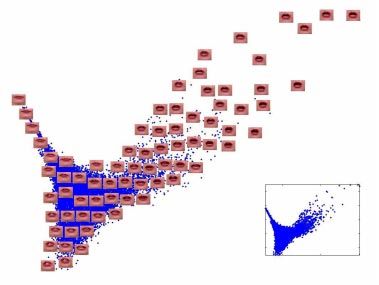
(D = 65664). Figure 7 shows the first two components of these images discovered by LLE with
K =24 nearest neighbors. These components appear to capture highly nonlinear degrees of freedom
associated with opening the mouth, pursing the lips, and clenching the teeth. Figure 8 shows how
one particular neighborhood of lip images is embedded in this two dimensional space. Dimension-
ality reduction of these images is useful for faster and more efficient animation. In particular, the
low dimensional outputs of LLE can be used to index the original collection of high dimensional
images. Fast and accurate indexing is an essential component of example-based video synthesis
from a large library of stored frames.
The data set of lip images is the largest data set to which we have applied LLE. LLE scales
relatively well to large data sets because it generates sparse intermediate results and eigenproblems.
Figure 9 shows the sparsity pattern of a large sub-block of the weight matrix Wi j for the data set of
lip images. Computing the twenty bottom eigenvectors (d = 20) for this embedding took only about
2.5 hours on a high end workstation, using specialized routines for finding eigenvectors of sparse,
symmetric matrices (Fokkema et al., 1998).
4. Implementation
The algorithm, as described in Figure 2, consists of three steps: nearest neighbor search (to identify
the nonzero elements of the weight matrix), constrained least squares fits (to compute the values
of these weights), and singular value decomposition (to perform the embedding). We now discuss
each of these steps in more detail.
126U NSUPERVISED LEARNING OF LOW DIMENSIONAL MANIFOLDS
Figure 5: Successful recovery of a manifold of known structure. Shown are the results of PCA
(top) and LLE (bottom), applied to N = 961 grayscale images of a single face translated
across a two dimensional background of noise. Such images lie on an intrinsically two
dimensional manifold, but have an extrinsic dimensionality equal to the number of pixels
in each image (D = 3009). Note how LLE (using K = 4 nearest neighbors) maps the
images with corner faces to the corners of its two dimensional embedding (d = 2), while
PCA fails to preserve the neighborhood structure of nearby images.
127S AUL AND ROWEIS
Figure 6: Images of faces mapped into the embedding space described by the first two coordinates
of LLE, using K = 12 nearest neighbors. Representative faces are shown next to circled
points at different points of the space. The bottom images correspond to points along the
top-right path, illustrating one particular mode of variability in pose and expression. The
data set had a total of N = 1965 grayscale images at 20×28 resolution (D = 560).
4.1 Step 1: Neighborhood Search
The first step of LLE is to identify the neighborhood of each data point. In the simplest formulation
of the algorithm, one identifies a fixed number of nearest neighbors, K, per data point, as measured
128U NSUPERVISED LEARNING OF LOW DIMENSIONAL MANIFOLDS
Figure 7: High resolution (D=65664) images of lips, mapped into the embedding space discovered
by the first two coordinates of LLE, using K = 24 nearest neighbors. Representative lips
are shown at different points in the space. The inset shows the first two LLE coordinates
for the entire data set (N = 15960) without any corresponding images.
Figure 8: A typical neighborhood of K =24 lip images mapped into the embedding space described
by the first two coordinates of LLE. The rectangle in the left plot locates the neighborhood
shown on the right in the overall space of lip images.
129S AUL AND ROWEIS
Figure 9: Sparsity pattern of the weight matrix Wi j for the data set of lip images. (Only a 1000×
1000 sub-block of the matrix is shown to reduce blurring of zero and nonzero elements
during printing.) Positive weights are indicated in blue; negative weights, in red. Roughly
99.85% of the elements are zero, although the ink density of the image above does not
reflect this accurately.
by Euclidean distance. Other criteria, however, can also be used to choose neighbors. For example,
one can identify neighbors by choosing all points within a ball of fixed radius. One can also use
locally derived distance metrics (based on a priori knowledge, estimated curvature, pairwise dis-
tances, or nonparametric techniques such as box counting) that deviate significantly from a globally
Euclidean norm. The number of neighbors does not have to be the same for each data point. In
fact, neighborhood selection can be quite sophisticated. For example, we can take all points within
a certain radius up to some maximum number, or we can take up to a certain number of neighbors
but none outside a maximum radius. In general, specifying the neighborhoods in LLE presents the
practitioner with an opportunity to incorporate a priori knowledge about the problem domain.
The results of LLE are typically stable over a range of neighborhood sizes. The size of that range
depends on various features of the data, such as the sampling density and the manifold geometry.
Several criteria should be kept in mind when choosing the number of neighbors per data point. First,
the algorithm can only be expected to recover embeddings whose dimensionality, d, is strictly less2
2. The K neighbors span a space of dimensionality at most K−1.
130U NSUPERVISED LEARNING OF LOW DIMENSIONAL MANIFOLDS
than the number of neighbors, K, and we have observed that some margin between d and K is gen-
erally necessary to obtain a topology-preserving embedding. (The exact relation between K and the
faithfulness of the resulting embedding remains an important open question.) Second, the algorithm
is based on the assumption that a data point and its nearest neighbors can be modeled as locally
linear; for curved data sets, choosing K too large will in general violate this assumption. Finally
in the unusual case where K > D (indicating that the original data is itself low dimensional), each
data point can be reconstructed perfectly from its neighbors, and the local reconstruction weights
are no longer uniquely defined. In this case, some further regularization must be added to break
the degeneracy.3 Figure 10 shows a range of embeddings discovered by the algorithm, all on the
same data set but using different numbers of nearest neighbors, K. The results are stable over a wide
range of values but do break down as K becomes too small or large.
The nearest neighbor step in LLE is simple to implement, though it can be time consuming for
large data sets (N ≥ 104 ) if performed without any optimizations. Computing nearest neighbors
scales in the worst case as O(DN 2 ), or linearly in the input dimensionality, D, and quadratically in
the number of data points, N. For many distributions of data, however—and especially for those
concentrated on a thin submanifold of the input space—constructions such as K-D trees or ball trees
can be used to compute the neighbors in O(N log N) time (Friedman et al., 1977; Gray and Moore,
2001; Moore et al., 2000; Omohundro, 1989, 1991). Recent work by Karger and Ruhl (2002)
specifically addresses the problem of computing nearest neighbors for data on low dimensional
manifolds. Efficient but approximate methods are also possible, some of which come with various
guarantees as to their accuracy (Indyk, 2000).
An implementation of LLE also needs to check that the graph formed by linking each data point
to its neighbors is connected. Efficient algorithms (Tarjan, 1972, 1983) exist for this purpose. If the
graph is disconnected (or weakly connected), then LLE should be applied separately to the data in
each of the graph’s (strongly) connected components; or else the neighborhood selection rule should
be refined to give a more strongly connected graph. In the disconnected or weakly connected case,
data from different connected components should be interpreted as lying on distinct data manifolds.
In theory, such situations could be detected after the fact by zeros in the eigenvalue spectrum (Perona
and Polito, 2002) of LLE.4 In practice, though, it seems much more straightforward to first compute
connected components and then apply LLE separately to each component. This not only reduces
the computational complexity of the algorithm, but also avoids any possible confounding of results
from different components.
4.2 Step 2: Constrained Least Squares Fits
The second step of LLE is to reconstruct each data point from its nearest neighbors. The optimal
reconstruction weights can be computed in closed form. Consider a particular data point ~x with K
nearest neighbors ~η j and reconstruction weights w j that sum to one. We can write the reconstruction
error as:
2 2
ε = ~x − ∑ j w j~η j = ∑ j w j (~x −~η j ) = ∑ jk w j wk G jk , (3)
3. A simple regularizer is to penalize the sum of the squares of the weights ∑ j Wi2j , which favors weights that are
uniformly distributed in magnitude. This is discussed further in Section 4.2.
4. The corresponding eigenvectors have constant values within each connected component, but different values in dif-
ferent components. This yields a zero embedding cost in Equation (2).
131S AUL AND ROWEIS
K=5 K=6 K=8 K = 10
K = 12 K = 14 K = 16 K = 18
K = 20 K = 30 K = 40 K = 60
Figure 10: Effect of neighborhood size on LLE. Embeddings of the two dimensional S-manifold
in the top panels of Figure 1, computed for different choices of the number of nearest
neighbors, K. A reliable embedding from D = 3 to d = 2 dimensions is obtained over a
wide range of values. If K is too small (top left) or too large (bottom right), however,
LLE does not succeed in unraveling the manifold and recovering the two underlying
degrees of freedom.
where in the first identity, we have exploited the fact that the weights sum to one, and in the second
identity, we have introduced the “local” Gram matrix,
G jk = (~x −~η j ) · (~x −~ηk ). (4)
By construction, this Gram matrix is symmetric and semipositive definite. The reconstruction error
can be minimized analytically using a Lagrange multiplier to enforce the constraint that ∑ j w j = 1.
In terms of the inverse Gram matrix, the optimal weights are given by:
∑k G−1
jk
wj = . (5)
∑lm G−1
lm
The solution, as written in Equation (5), appears to require an explicit inversion of the Gram matrix.
In practice, a more efficient and numerically stable way to minimize the error (which yields the
132U NSUPERVISED LEARNING OF LOW DIMENSIONAL MANIFOLDS
0.25 0 0.5
0.25 0.5 0
0.25 0.5 0
0.25 0 0.5
Figure 11: Degeneracy of reconstruction weights. If there are more neighbors (K) than input di-
mensions (D), then the weights which minimize the reconstruction error in Equation (1)
do not have a unique solution. Consider, for example, a two dimensional data point
whose four neighbors lie at the corners of a diamond. In this case, many different set-
tings of the weights lead to zero reconstruction error. Three possible settings are shown
above. Adding a regularizer that penalizes the squared magnitude of the weights favors
the left solution over all others. Note that while this example has particular symmetries
(chosen for ease of visualization), the degeneracy arises whenever K >D, even for points
in general position.
same result as above) is simply to solve the linear system of equations, ∑k G jk wk = 1, and then to
rescale the weights so that they sum to one.
In unusual cases, it can arise that the Gram matrix in Equation (4) is singular or nearly singular—
for example, for example, when there are more neighbors than input dimensions (K > D), or when
the data points are not in general position. In this case, the least squares problem for finding the
weights does not have a unique solution (see Figure 11), and the Gram matrix must be conditioned
(before solving the linear system) by adding a small multiple of the identity matrix,
∆2
G jk ← G jk + δ jk Tr(G),
K
where δ jk is 1 if j = k and 0 otherwise, Tr(G) denotes the trace of G, and ∆2
1. This amounts to
adding a regularization term to the reconstruction cost that measures the summed squared magnitude
of the weights. (One can also consider the effect of this term in the limit ∆ → 0.)
The regularization term acts to penalize large weights that exploit correlations beyond some
level of precision in the data sampling process. It may also introduce some robustness to noise
and outliers. This form of regularization (with ∆ = 0.1) was used, for example, to compute all
the embeddings in Figure 1. For these synthetic manifolds, the regularization is essential because
there are more neighbors (K = 8) than input dimensions (D = 3). (For most real data sets requiring
dimensionality reduction, however, D is much larger than K.)
Computing the reconstruction weights Wi j is typically the least expensive step of the LLE algo-
rithm. The computation scales as O(DNK 3 ); this is the number of operations required to solve a
K×K set of linear equations for each data point. It is linear in both the number of data points and the
number of input dimensions. The weight matrix can be stored as a sparse matrix with NK nonzero
133S AUL AND ROWEIS
elements. The inputs ~Xi do not all need to be in memory at once for this step because the algorithm
fills in the weights based on a purely local computation.
4.3 Step 3: Eigenvalue Problem
The final step of LLE is to compute a low dimensional embedding based on the reconstruc-
tion weights Wi j of the high dimensional inputs ~Xi . Note that only information captured by the
weights Wi j is used to construct an embedding; the actual inputs ~Xi do not appear anywhere in the
final step of the algorithm (and hence do not need to remain in memory once the weights are com-
puted). The low dimensional outputs ~Yi are found by minimizing the cost function, Equation (2),
for fixed weights Wi j . This cost function is minimized when the outputs ~Yi are reconstructed (or
nearly reconstructed) by the same weighted linear combinations of neighbors as computed for the
inputs. Note that the assignment of neighbors is always based on the locations of the inputs ~Xi ; the
algorithm does not dynamically recompute neighbors based on the locations of the outputs ~Yi .
To optimize the embedding cost function in Equation (2), we rewrite it as the quadratic form:
Φ(Y ) = ∑ Mi j (~Yi ·~Y j ), (6)
ij
involving inner products of the outputs ~Yi . The square N ×N matrix M that appears in Equation (6)
is given by:
Mi j = δi j −Wi j −W ji + ∑ WkiWk j . (7)
k
The matrix M is sparse, symmetric, and semipositive definite.
The optimization of Equation (6) is performed subject to constraints that make the problem well
posed. Note that we can translate the outputs ~Yi by a constant displacement without affecting the
cost, Φ(Y ), in Equation (2). We remove this translational degree of freedom by requiring the outputs
to be centered on the origin:
∑~Yi = ~0. (8)
i
We can also rotate the outputs ~Yi without affecting the cost, Φ(Y ), in Equation (2). To remove this
rotational degree of freedom—and to fix the scale—we constrain the ~Yi to have unit covariance, with
outer products that satisfy
1 ~~>
N∑
YiYi = I, (9)
i
where I is the d×d identity matrix. This constraint that the output covariance be equal to the identity
matrix embodies three assumptions: first, that the different coordinates in the embedding space
should be uncorrelated to second-order; second, that reconstruction errors for these coordinates
should be measured on the same scale; and third, that this scale should be of order unity. (Note
that these assumptions are rather mild. Since we are free to rotate and homogeneously rescale
the outputs, we can always make the covariance of ~Y to be diagonal and of order unity. Further
restricting the covariance to be the identity matrix only introduces the additional assumption that all
the embedding coordinates should be of the same scale.)
Under these restrictions, the optimal embedding—up to a trivial global rotation of the embed-
ding space—is found by minimizing Equation (2) subject to the constraints in Equations (8–9). This
can be done in many ways, but the most straightforward is to find the bottom d+1 eigenvectors of
134U NSUPERVISED LEARNING OF LOW DIMENSIONAL MANIFOLDS
the cost matrix, M. (The “bottom” or “top” eigenvectors are those corresponding to the smallest or
largest eigenvalues.) This equivalence between the optimization of a normalized quadratic form and
the computation of largest or smallest eigenvectors is a version of the Rayleitz-Ritz theorem (Horn
and Johnson, 1990). The optimization is performed by introducing Lagrange multipliers to enforce
the constraints in Equations (8–9). Setting the gradients with respect to the vectors ~Yi to zero leads to
a symmetric eigenvalue problem, exactly as in derivations of principal component analysis (Bishop,
1996). The eigenvector computation in LLE also has the same form as the eigenvector computation
for image segmentation by normalized cuts (Shi and Malik, 2000). The bottom eigenvector of the
matrix, M, which we discard, is the unit vector with all equal components; it represents the free
translation mode of eigenvalue zero. Discarding this eigenvector enforces the constraint in Equa-
tion (8) that the outputs have zero mean, since the components of other eigenvectors must sum to
zero, by virtue of orthogonality with the bottom one. The remaining d eigenvectors constitute the
d embedding coordinates found by LLE.
Note that the bottom d+1 eigenvectors of the sparse, symmetric matrix M can be found without
performing a full matrix diagonalization (Bai et al., 2000). Operations involving M can also exploit
its representation as the product of two sparse matrices,
M = (I −W )> (I −W ),
giving substantial computational savings for large values of N. In particular, left multiplication
by M (the subroutine required by most sparse eigensolvers) can be performed as:
M~v = (~v −W~v) −W > (~v −W~v),
requiring just one multiplication by W and one multiplication by W > . Thus, the matrix M never
needs to be explicitly created or stored; it is sufficient just to store and multiply by the (even sparser)
matrix W . An efficient implementation of the multiplication ~v ← M~v can be achieved using the
update ~v ←~v −W~v followed by the update ~v ←~v −W >~v.
The final step of LLE is typically the most computationally expensive. Without special opti-
mizations, computing the bottom eigenvectors scales as O(dN 2 ), linearly in the number of embed-
ding dimensions, d, and quadratically in the number of data points, N. Specialized methods for
sparse, symmetric eigenproblems (Bai et al., 2000; Fokkema et al., 1998), however, can be used to
reduce the complexity to subquadratic in N. For very large problems, one can consider alternative
methods for optimizing the embedding cost function, such as direct descent by conjugate gradi-
ent methods (Press et al., 1993), iterative partial minimizations, Lanczos iterations, or stochastic
gradient descent (LeCun et al., 1998).
Note that the dth coordinate output by LLE always corresponds to the (d + 1)st smallest eigen-
vector of the matrix M, regardless of the total number of outputs computed or the order in which
they are calculated. Thus, for efficiency or convenience, we can compute the bottom eigenvectors of
Equation (7) one at a time, yielding a “nested” set of embeddings in successively higher dimensions.
5. Extensions
In this section, we describe several useful extensions to the basic LLE algorithm, including the
handling of input in the form of pairwise distances, the use of convex reconstructions, and the
estimation of a manifold’s underlying dimensionality.
135S AUL AND ROWEIS
5.1 LLE from Pairwise Distances
The LLE algorithm, as described in Figure 2, takes as input the N high dimensional vectors, ~Xi . In
many settings, however, the user may not have access to data of this form, but only to measurements
of dissimilarity or distance between data points. A simple variation of LLE can be applied to input
of this form. In this way, matrices of pairwise distances can be analyzed by LLE just as easily as by
MDS (Cox and Cox, 1994) or other distance-based approaches to dimensionality reduction (Tenen-
baum et al., 2000).
To derive the reconstruction weights for each data point, we need to compute the Gram matrix
G jk between its nearest neighbors, as defined by Equation (4). This matrix can be found by inferring
dot products from pairwise distances in exactly the same manner as MDS. In particular, consider
a point ~x and its K neighbors ηi , and let Si j denote the symmetric square matrix, of size (K +1)×
(K+1), that records pairwise squared distances between these points. (In a slight abuse of notation,
here we will allow the indices to range from i, j = 0, 1, . . . , K, where positive values refer to the K
neighbors of ~x and the zero index refers to the point ~x itself.) For the purpose of computing the
Gram matrix G in Equation (4), we can assume without loss of generality that these K+1 points are
centered on the origin. In this case, their dot products ρi j are given exactly in terms of their pairwise
squared distances Si j by:
" K 2 K #
1 1 1
ρi j =
2 K+1 k=0 ∑ (Sik + Sk j ) − K+1 ∑ Sk` − Si j .
k,`=0
In terms of our earlier notation, the elements in this matrix store the dot products ρ00 = |~x|2 , ρ0 j =
~x · ~η j (for j > 0), and ρi j = ~ηi · ~η j (for i, j > 0). The elements of the “local” Gram matrix Gi j are
given in terms of these dot products ρi j by:
Gi j = (~x −~ηi) · (~x −~η j ) = ρ00 − ρi0 − ρ0 j + ρi j .
Note that Gi j is a K ×K square matrix, whereas ρi j is one dimension larger. In terms of the Gram
matrix Gi j , the reconstruction weights for each data point are given by Equation (5). The rest of the
algorithm proceeds as usual.
Note that this variant of LLE does not in fact require the complete N ×N matrix of pairwise
distances. Instead, for each data point, the user needs only to specify the nearest neighbors, the
distances to neighbors, and the pairwise distances between neighbors. This information can be
conveniently stored in a sparse matrix. The first step of the algorithm remains to identify nearest
neighbors; these can be identified, for example, by the K smallest non-missing elements of each
row in the given distance matrix.
It is natural to wonder if this variant of LLE could succeed with the user specifying even
fewer elements in the matrix of pairwise distances. Figure 12 shows that just preserving the
pairwise distances between nearest neighbors is not in general sufficient to recover an underlying
manifold. Consider the three dimensional data set whose points have integer coordinates satisfy-
ing x + y + z = 0; that is, they lie at the sites of a planar square lattice. Suppose that points with even
x-coordinates are colored black and those with odd x-coordinates are colored white. The degenerate
“two point” embedding that maps all black points to the origin and all white points one unit away
exactly preserves the distance between each point and its four nearest neighbors. Nevertheless, this
embedding completely fails to preserve the structure of the underlying manifold.
136U NSUPERVISED LEARNING OF LOW DIMENSIONAL MANIFOLDS
Figure 12: Preserving just the distances to nearest neighbors is not sufficient to recover the under-
lying manifold. Shown above is a trivial “two-point” embedding that exactly preserves
the distances between each point and its four nearest neighbors without revealing the
two dimensional structure of the data.
5.2 Convex Reconstructions
The rows of the weight matrix Wi j computed by the second step of LLE are constrained to sum to
one but may be either positive or negative. In simple geometric terms, this constraint forces the
reconstruction of each data point to lie in the subspace spanned by its nearest neighbors; the optimal
weights compute the projection of the data point into this subspace. One can additionally constrain
these weights to be nonnegative, thus forcing the reconstruction of each data point to lie within
the convex hull of its neighbors. It is more expensive to compute the least squares solution with
nonnegativity constraints, but the additional cost is usually negligible compared to the other two
steps of LLE.5 In conjunction with the sum-to-one constraint, the constraint of nonnegativity limits
the weights strictly to the range [0,1]. Such a constraint has both advantages and disadvantages.
On one hand, it tends to increase the robustness of linear fits to outliers. On the other hand, it can
degrade the reconstruction of data points that lie on the boundary of a manifold and outside the
convex hull of their neighbors. For such points, negative weights may be helpful.
A general prescription for using convex versus linear reconstructions does not exist to cover all
applications of LLE. In certain applications, it may be straightforward to certify that neighborhoods
are free of outliers, thus minimizing the dangers of unbounded weights; in others, it may be sim-
pler to choose K nearest neighbors everywhere and and require convex reconstructions. A useful
heuristic is to inspect a histogram of the reconstruction weights obtained without nonnegativity con-
straints. If certain data points have very large (positive or negative) reconstruction weights, it may
be wise to re-assign their neighbors or to constrain their linear reconstructions to be convex. In our
5. In particular, one must solve a problem in quadratic programming: minimize ∑ jk w j wk G jk from Equation (3) subject
to ∑ j w j =1 and w j ≥0. The required optimization is convex, with solutions that often lie on the edge of the constraint
region (Judge and Takayama, 1966).
137S AUL AND ROWEIS
applications of LLE to images and other data sets, these warning signals did not arise. Thus, in our
general experience, we have not found the extra constraint of convexity to be especially necessary
for well-sampled data.
5.3 Estimating the Intrinsic Dimensionality, d
Given data sampled from an underlying manifold, it is naturally of interest to estimate the mani-
fold’s intrinsic dimensionality, d. Recall how PCA solves this problem for linear subspaces: the
dimensionality is estimated by the number of eigenvalues of the sample covariance matrix compa-
rable in magnitude to the largest eigenvalue. An analogous strategy for LLE (Perona and Polito,
2002) immediately suggests itself—that is, to estimate d by the number of eigenvalues compara-
ble in magnitude to the smallest nonzero eigenvalue of the cost matrix, M, from Equation (7). In
practice, however, we have found this procedure to work only for contrived examples, such as data
that lies on an essentially linear manifold, or data that has been sampled in an especially uniform
way (so that the lowest nonzero eigenvalues are equal or nearly equal due to symmetry). More
generally, we have not found it to be reliable. Figure 13 plots the eigenvalue spectrum of the cost
matrix in Equation (7) for several data sets of intrinsic dimensionality d = 2. The eigenvalues reveal
a distinguishing signature at d = 2 in some of these plots, but not in others.
We have found it more useful to rely on classical methods (Pettis et al., 1979) for estimating
the intrinsic dimensionality d of a data set. One way to estimate this dimensionality is by examin-
ing the eigenvalue spectra of local covariance matrices. Performing in essence a local PCA in the
neighborhood of each data point, we can then ask whether these analyses yield a consistent estimate
of the intrinsic dimensionality. Yet another estimate can be obtained by box-counting. Suppose we
consider two points to be neighbors if they lie within a distance, ε. If the data are uniformly sam-
pled over the manifold, then the number of neighbors should scale for small ε as Kε ∝ εd , where d
is the intrinsic dimensionality. Recently, robust variations on this basic idea have been developed
to estimate the intrinsic dimensionality of finite data sets with noise and several degrees of free-
dom (Brand, 2003; Kegl, 2003). Both these methods can be used prior to the final step of LLE to
set the number of embedding coordinates computed by the algorithm.
5.4 Enforcing the Intrinsic Dimensionality, d
LLE normally computes an ordered set of embedding coordinates without assuming the particular
number that will be used. In some applications, however, a manifold’s intrinsic dimensionality
may be known a priori, or the user may wish to bias the results of LLE toward an embedding
of a particular dimensionality (such as d = 2, which is easily visualized). In these circumstances,
the second step of LLE can be modified in a simple way to suppress spurious or noisy degrees of
freedom and force a desired intrinsic dimensionality, d. For each data point, the idea is to project
its neighbors into their d-dimensional subspace of maximal variance before performing the least
squares reconstruction. The subspace is computed from the d dominant eigenvectors of the Gram
matrix G in Equation (4). The effect of this projection is to limit the rank of G before solving for the
reconstruction weights. (Note that this is a far better way to limit the rank of the Gram matrix than
simply reducing the number of nearest neighbors.) The reconstruction weights are then computed
as before, but from the rank-limited Gram matrix (and using the minimum norm solution to the least
squares problem).
138U NSUPERVISED LEARNING OF LOW DIMENSIONAL MANIFOLDS
-1 -3
10 10
-3 -4
10 10
λ
n
-5 -5
10 10
-7 -6
10 10
1 2 3 4 5 6 1 2 3 4 5 6
n n
-5 -5
10 10
-6
10
-7
10
λ
n
-8
10
-9
10
-10 -10
10 10
1 2 3 4 5 6 1 2 3 4 5 6
n n
Figure 13: Eigenvalues from the third step of LLE are not reliable indicators of intrinsic dimen-
sionality. Plots show the smallest nonzero eigenvalues λn of the embedding cost matrix
in Equation (7) for several data sets. The gap between the n = 2 and n = 3 eigenvalues
reveals the true dimensionality (d = 2) of regularly sampled data in the plane and on the
sphere. There is no similar signature, however, for the randomly sampled data on the
two bottom manifolds.
As an example of this method, Figure 14 shows the results of applying LLE to scanned images
of handwritten digits from the USPS data set (Hull, 1994). The digits (ZERO through NINE) were
taken from zip codes on Buffalo postal envelopes. The images were preprocessed by downsampling
to 16×16 resolution (D = 256) and quantizing the grayscale intensity to 256 levels. The inputs ~Xi to
LLE were the raw pixel values. For the results in Figure 14, neighbors were projected into an eight
139S AUL AND ROWEIS
9 7
4
2
y2
y2
y2
0 3 6 5
8
1
y1 y1 y1
8
8
5
y5
y7
y7
5
5 8
y3 y3 y1
Figure 14: Embeddings of N = 11000 handwritten digits from K = 18 nearest neighbors per digit.
The inputs ~Xi were grayscale images of handwritten numerals (ZERO through NINE)
taken from the USPS data set (Hull, 1994) at 16×16 resolution (D = 256) A maximum
manifold dimensionality of d = 8 was enforced by singular value decomposition of the
local Gram matrices, as described in Section 5.4. The top panels show the first two
coordinates discovered by LLE. Many digit classes (labelled) are well clustered in just
these two dimensions. Classes that overlap in the first two dimensions are typically
separated in others, as the bottom panels show for FIVES versus EIGHTS in the third,
fifth and seventh LLE coordinates.
dimensional subspace (d = 8) before performing the least squares reconstructions and computing
the weights Wi j . Interestingly, the resulting embedding provides a low dimensional clustering of the
handwritten digits, even though LLE did not itself make use of the labels distinguishing different
digits. Note that digit classes confounded in certain projections are often separated in others. En-
forcing the dimensionality of d = 8 is not essential for this effect; it is interesting to see, however,
that this number does yield an accurate clustering, with the higher-order coordinates discovered by
LLE playing as important a role as the first and second.
140U NSUPERVISED LEARNING OF LOW DIMENSIONAL MANIFOLDS
6. From embeddings to mappings
LLE provides an embedding for the fixed set of training data to which the algorithm is applied.
Often, however, we need to generalize the results of LLE to new locations in the input space. For
example, suppose that we are asked to compute the output ~y corresponding to a new input ~x. In
principle, we could rerun the entire LLE algorithm with the original data set augmented by the new
input. For large data sets of high dimensionality, however, this approach is prohibitively expensive.
For the purposes of generalization, it is therefore useful to derive an explicit mapping between the
high and low dimensional spaces of LLE that does not require an expensive eigenvector calculation
for each query. A natural question is how to construct such a mapping given the results of LLE
from a previous run of the algorithm. In this section, we describe two possible solutions—one
non-parametric, one parametric—to this problem.
6.1 Non-parametric Model
The non-parametric solution relies on a natural mapping between the low and high dimensional
spaces of LLE. In particular, to compute the output ~y for a new input ~x, we can do the following: (i)
identify the K nearest neighbors of ~x among the training inputs; (ii) compute the linear weights w j
that best reconstruct ~x from its neighbors, subject to the sum-to-one constraint, ∑ j w j = 1; (iii)
output ~y = ∑ j w j~Y j , where the sum is over the outputs corresponding to the neighbors of ~x. A
non-parametric mapping from the embedding space to the input space can be derived in the same
manner: to compute the input ~x for a new output ~y, identify the nearest neighbors of ~y among the
training outputs, compute the analogous reconstruction weights, and output ~x = ∑ j w j ~X j . (Note that
in this direction, moreover, there does not exist the option of rerunning LLE on an augmented data
set.)
To evaluate the usefulness of this non-parametric mapping, we investigated LLE as a front
end for statistical pattern recognition. Dimensionality reduction is often used as a form of feature
extraction to simplify or accelerate other algorithms in machine learning. We compared the features
produced by LLE to those of PCA for a benchmark problem in handwritten digit recognition. The
raw data were images of handwritten digits from the USPS database, as described in Section 5.4.
Half the images (5500 examples, 550 per digit) was used for training, and the other half for testing.
On test images, LLE features were computed by nearest-neighbor interpolation from the training
images (as described above), while PCA features were computed by subtracting the mean of the
training images then projecting onto their principal components.
Two simple classifiers were implemented: a K-nearest-neighbor classifier—with K chosen to
optimize leave-one-out performance on the training set—and a log-linear classifier obtained from
multiclass logistic regression (or softmax regression) (Bishop, 1996). The parameters of the softmax
regression were set to maximize the conditional log likelihood of the training set. As features for
these classifiers, we used either the first d coordinates discovered by LLE on the entire (unlabeled)
training set of 5500 images, or else the projection onto the first d principal components of the
training data, as computed by running PCA on the training set (i.e. subtracting the sample mean
and finding the leading eigenvectors of the sample covariance matrix). LLE was run using K = 18
nearest neighbors per data point to compute the reconstruction weights.
Figure 15 shows the results of these experiments. For small numbers of features, LLE leads
to significantly lower error rates than PCA on both the training and test sets (though only the test
error rates are shown in the figure). These results suggest that nearest-neighbor interpolation is an
141You can also read