DeepMerge II: Building Robust Deep Learning Algorithms for Merging Galaxy Identification Across Domains

MNRAS 000, 1–17 (2021) Preprint 3 March 2021 Compiled using MNRAS LATEX style file v3.0

 DeepMerge II: Building Robust Deep Learning Algorithms for Merging
 Galaxy Identification Across Domains
 A. Ćiprijanović,1★ D. Kafkes,1 K. Downey,2 S. Jenkins,2 G. N. Perdue,1 S. Madireddy,3 T. Johnston,4
 G. F. Snyder,5 B. Nord1,2,6
 1 Fermi National Accelerator Laboratory, P.O. Box 500, Batavia, IL 60510, USA
 2 Department of Astronomy and Astrophysics, University of Chicago, IL 60637, USA
 3 Argonne National Laboratory, 9700 S Cass Ave, Lemont, IL 60439, USA
 4 Oak Ridge National Laboratory, 1 Bethel Valley Rd, Oak Ridge, TN 37830, USA
arXiv:2103.01373v1 [astro-ph.IM] 2 Mar 2021

 5 Space Telescope Science Institute, 3700 San Martin Drive, Baltimore, MD 21218, USA
 6 Kavli Institute for Cosmological Physics, University of Chicago, Chicago, IL 60637, USA

 Accepted XXX. Received YYY; in original form ZZZ

 ABSTRACT
 In astronomy, neural networks are often trained on simulation data with the prospect of being used on telescope observations.
 Unfortunately, training a model on simulation data and then applying it to instrument data leads to a substantial and potentially
 even detrimental decrease in model accuracy on the new target dataset. Simulated and instrument data represent different data
 domains, and for an algorithm to work in both, domain-invariant learning is necessary. Here we employ domain adaptation
 techniques— Maximum Mean Discrepancy (MMD) as an additional transfer loss and Domain Adversarial Neural Networks
 (DANNs)— and demonstrate their viability to extract domain-invariant features within the astronomical context of classifying
 merging and non-merging galaxies. Additionally, we explore the use of Fisher loss and entropy minimization to enforce better
 in-domain class discriminability. We show that the addition of each domain adaptation technique improves the performance
 of a classifier when compared to conventional deep learning algorithms. We demonstrate this on two examples: between two
 Illustris-1 simulated datasets of distant merging galaxies, and between Illustris-1 simulated data of nearby merging galaxies and
 observed data from the Sloan Digital Sky Survey. The use of domain adaptation techniques in our experiments leads to an increase
 of target domain classification accuracy of up to ∼20%. With further development, these techniques will allow astronomers to
 successfully implement neural network models trained on simulation data to efficiently detect and study astrophysical objects in
 current and future large-scale astronomical surveys.
 Key words: galaxies: interactions, methods: data analysis, methods: statistical, techniques: image processing

 1 INTRODUCTION vance the study of merging galaxies (Ackermann et al. 2018; Snyder
 et al. 2019; Pearson et al. 2019; Ćiprijanović et al. 2020), improving
 Studies of galaxy mergers are crucial for understanding the evolution
 both the quality of the results and the speed of working with big
 of galaxies as astronomical objects, their star formation rates, chem-
 datasets. Studies of merging galaxies using machine learning can
 istry, particle acceleration and other properties. Moreover, they are
 greatly benefit from models trained on simulated data, which can
 equally important for cosmology, understanding structure formation
 then be successfully applied to newly observed images from present
 and the study of evolution of matter in the universe. Being able to
 and future large-scale surveys.
 leverage large samples of merging galaxies and to connect the knowl-
 Simulated and observed images have different origins and repre-
 edge obtained from large-scale simulations and astronomical surveys
 sent different data domains. In this case, labeled simulation images
 will play an important role in these studies.
 represent the source domain we are starting from, while observed
 Standard methods for classifying merging galaxies using visual in-
 data (often unlabeled) is the target domain. While images produced
 spection (Lin et al. 2004) or extraction of parametric measurements
 by simulations are made to mimic real observations from a particular
 of structure such as the Sérsic index (Sérsic 1963), Gini coefficient,
 telescope, unavoidable small differences can cause the model trained
 M20 – the second-order moment of the brightest 20% percent of
 on simulated images to perform substantially worse when applied
 the galaxy’s flux (Lotz et al. 2004), CAS – Concentration, Asymme-
 to real data. This substandard performance has been demonstrated
 try, Clumpiness (Conselice et al. 2003) etc., can be time consuming,
 directly in the case of merging galaxies by Ćiprijanović et al. (2020).
 prone to biases, or require the use of high-quality images. Due to these
 The authors show that even when the only difference between the two
 limitations, it has been shown that machine learning can greatly ad-
 merging galaxy datasets is the inclusion of noise, convolutional neu-
 ral networks (CNNs) trained on one dataset cannot classify the other
 ★
 dataset at all. In the paper the classification accuracy of in-domain
 E-mail: aleksand@fnal.gov

 © 2021 The Authors

2 A. Ćiprijanović et al.
images was 79%, while the accuracy for out-of-domain images was (source) and with (target) the addition of random sky shot noise to
around 50%, equivalent to random guessing. Additionally, Pearson mimic observations from the Hubble Space Telescope.
et al. (2019) use a dataset from the EAGLE simulation (Schaye et al. Additionally, we test these methods on a harder and more realistic
2015), which is made to mimic Sloan Digital Sky Survey (SDSS) application example, where the source domain includes simulated
observations, and real SDSS images (Lintott et al. 2008; Darg et al. galaxies at = 0 from the Illustris-1 simulation (Vogelsberger et al.
2010). Their work provides further evidence that the performance of 2014) made to mimic SDSS observations and real SDSS images of
the classifier trained on one dataset has much lower accuracy when merging galaxies (Lintott et al. 2008; Darg et al. 2010). These two do-
classifying the other dataset. They achieve out-of-domain accuracies mains exhibit a much larger discrepancy, and simply applying MMD
between 53 − 65%, with the classifier trained on real SDSS im- and adversarial training does not perform well. We demonstrate that
ages classifying EAGLE simulation images performing particularly combining MMD with transfer learning from the model trained on
poorly. These two examples are indicative of a great need for more the first dataset of distant merging galaxies can be used to solve this
sophisticated deep learning methods to be applied to cross-domain harder domain adaptation problem.
studies in astrophysical contexts. With the use of domain adaptation techniques mentioned above,
 An important area of deep learning research includes the develop- we manage to increase the target domain classification accuracy up to
ment of Domain Adaptation (DA) techniques (Csurka 2017; Wang ∼20% in our experiments, which allowed the model to be successfully
& Deng 2018; Wilson & Cook 2020). They allow the model to used in both domains. It is our hope that the use and continued devel-
learn the invariant features shared between the domains and align opment of these techniques will allow astronomers and cosmologists
the extracted latent feature distributions. This allows the model to to develop deep learning algorithms that can combine information
successfully find the decision boundary that distinguishes between from either simulations and real data, or to combine observations
different classes in multiple domains at the same time. One group of from different telescopes.
divergence-based DA methods includes finding and minimizing some The remainder of the paper is structured as follows: In Section 2,
divergence criterion between the source and target data distributions. we introduce and explain the domain adaptation methods used in this
Some of the most well known methods include Maximum Mean paper. We explain the neural network architectures we use in Sec-
Discrepancy (MMD; Gretton et al. (2012b)), Correlation Alignment tion 3. In Section 4, we give details about the images we use in our
(CORAL; Sun & Saenko (2016); Sun et al. (2016)), Contrastive Do- experiments and talk more about the experimental setup in Section 5.
main Discrepancy (CDD; Kang et al. (2019)), and the Wasserstein Finally, our results are given in Section 6, followed by a discussion
metric (Shen et al. 2018). On the other hand, adversarial-based DA in Section 7.
methods use either generative models (Liu & Tuzel 2016) to create
synthetic target data related to the source domain or more simple
models that utilize domain-confusion loss (Ganin et al. 2016), which 2 METHODS
measures how well the model distinguishes between different data
domains. Deep learning is already bringing advances in astronomy and survey
 In this paper we employ two different domain adaptation science, as in other academic fields and industry. Many astronomi-
techniques— Maximum Mean Discrepancy (MMD) and domain ad- cal applications often require these models to perform well on new
versarial training with a domain-confusion loss— to improve cross- datasets, requiring the applicability of features learned from simu-
domain applications of deep learning models to the problem of dis- lations to data that the model was not initially trained on, including
tinguishing between merging and non-merging galaxies. Maximum newly available observed data and cross-telescope applications. Since
Mean Discrepancy works by minimizing a distance measure of the labelling new data is slow and prone to errors, retraining these neu-
mean embeddings of the two domain distributions in latent feature ral networks on new datasets in order to maintain high performance
space (Gretton et al. 2012b). It is applied to standard classifica- is often impractical. In these situations, a discriminative model that
tion networks as a transfer loss. Domain adversarial neural networks is able to transfer knowledge between training (source domain) and
(DANNs; Ganin et al. (2016)), use adversarial training between a la- new data (target domain) is necessary. This can be achieved by using
bel classifier— which distinguishes mergers from non-mergers— and domain adaptation techniques, which extract invariant features be-
a domain classifier— which classifies the source and target domain of tween two domains, so that a neural network classifier trained on the
images. This kind of training employs a gradient reversal layer within source domain can also be applied successfully on a target domain.
the domain classifier, thereby maximizing the loss in this branch and As previously underscored, this functionality is very useful in situa-
leading to the extraction of domain-invariant features from both sets tions often found in astronomy, where the target domain is comprised
of images. Following methods from Zhang et al. (2020a), we also add of new observational data that has very few identified objects or is
Fisher loss and entropy minimization (Grandvalet & Bengio 2005), completely unlabeled. Here we will test several DA techniques that
which can be used as additional losses for both MMD or domain can be effective in the situation where the target domain is unlabeled.
adversarial training, to improve the overall performance of the clas- These techniques include adding transfer loss to the widely-adopted
sifier. Both of these loss functions enforce additional discriminability cross-entropy loss used for standard classification of images.
between the classes in source (Fisher loss) and target (entropy mini- Cross-entropy loss is given as:
mization) domains, by producing more compact classes in the latent M
 ∑︁
feature space. LCL = − log ( ), (1)
 We test two networks for a comparison of technique results across =1
architectures: DeepMerge, a simple convolutional network for clas- where is a particular class and the total number of classes is M.
sification of galaxies presented in Ćiprijanović et al. (2020), as well The true label for class is given as , and ( ) is the neural
as the more complex and well-known ResNet18 (He et al. 2015). We network assigned score, i.e. the output prediction from the last layer,
demonstrate both methods on a dataset similar to the one from Ćipri- for a given class . Minimizing cross-entropy loss leads to output
janović et al. (2020), using simulated distant merging galaxies from predictions approaching real label values, which results in an increase
Illustris-1 (Vogelsberger et al. 2014) at redshift z = 2, both without in classification accuracy.

MNRAS 000, 1–17 (2021)

DeepMerge II: Building Robust Deep Learning Algorithms for Merging Galaxy Identification Across Domains 3
 The inclusion of transfer loss allows DA techniques to impact t are random variables drawn from Ps and Pt respectively, function
the way the network learns via backpropagation. We explore two class F closely resembles the set of CDF functions in vector space
different transfer losses in this paper: Maximum Mean Discrepancy with total variance less than one operating on the domain (−∞, IR]
(MMD; Gretton et al. (2012a)) and using the loss of the discriminator and the supremum is the least element in F greater than or equal to the
from a Domain Adversarial Neural Network (DANN; Ganin et al. chosen , i.e. the max of the subset. By this definition, if Ps = Pt , then
(2016)). Additionally, we explore adding Fisher loss (Zhang et al. (Ps , Pt , F ) = 0 (Gretton et al. 2012a; Pan et al. 2011). If Ps ≠ Pt ,
2020a), which enforces feature discriminability between classes in then there must exist some such that the distance between the
the source domain, and entropy minimization, which forces a target two means is maximized. This becomes an optimization problem in
sample to move toward one of the compacted and separated source which the criterion aims to maximize the discrepancy by separating
classes (Grandvalet & Bengio 2005), leading to better class separa- the two distributions as far as possible in some high-dimensional
bility in the target domain. feature space. Kernel methods are well suited to this task since they
 The resultant total classifier loss (Zhang et al. 2020a) has multiple are able to map means into higher-dimensional Reproducing Kernel
components: Hilbert Spaces (RKHSs). Furthermore, this embedding linearizes the
 metric by mapping the input space into a feature vector space.
LTOT = LCL + FL LFL + EM LEM + TL LTL , (2)
 RKHSs possess several properties that facilitate the calculation
where we define LTOT , LCL , LFL , LEM , LTL as total loss, classi- of , including a property of norms that rescale the output of a
fier loss, Fisher loss, entropy minimization, and transfer loss, respec- function to fit within a unit ball— which greatly restricts the many
tively. The contribution of these additional losses can be weighted possibilities of function class F — and a reproducing property that
using weights FL , EM and TL . Further details about the different reduces calculations to the inner product of the output of functions.
losses used are given below. For example, h , ( , ·)i = ( ), where ( , ·) is a kernel that has one
 argument fixed at , and the second free. Performing this calculation
 in an RKHS means there is no need to explicitly calculate the mapping
2.1 Transfer Loss function ( ) that maps s and t into an RKHS feature space due to
The transfer loss LTL is calculated from the DA technique, whose equivalence between ( ) and ( , ·) : h ( ), ( 0 )i = h ( , 0 )i =
goal is to decrease discrimination between the source and the target h ( , ·), ( 0 , ·)i. Therefore, Eq. 3 can be re-expressed as two inner
domains. This involves the representation of data from both domains products with kernels mean embeddings in an RKHS:
in a higher-dimensional latent feature space. In this paper, we explore
 (Ps , Pt , F ) := sup E Ps [h ( s ), i] − sup E Pt [h ( t ), i]
the use of both MMD and domain adversarial training as transfer cri- | | | | ≤1 | | | | ≤1
teria. MMD frames the domain problem in terms of high-dimensional (4)
statistics and involves calculating the distance between the mean em-
beddings of the source and target domain distributions. In the case = sup h s , i − sup h t , i = sup h s − t , i,
of adversarial training, the domain discrepancy problem is addressed
by adopting DANN, a neural network that seeks to find the common where s and t are the source and target distribution’s mean embed-
feature space between the source and target distributions by jointly dings and is still bounded by the unit ball of the RKHS. Clearly,
minimizing the training loss in the source domain while maximizing the inner product is maximized for the identity h , i = 1. Therefore,
the loss of the domain classifier. to maximize the mean discrepancy we need = s - t , leaving us
 We will denote the source and target domains as Ds and Dt re- with the final formula:
spectively. Source domain images are labeled, so we have s pairs
 (Ps , Pt , F ) := E Ps [ ( s , s0 )] − 2E Ps,t [ ( s , t )] + E Pt [ ( t , t0 )],
of images and labels {xs , ys }, while in the case of the target domain
we have t unlabeled images xt . Images from both domains are as- (5)
sociated with domain labels ds for source domain and dt for target where all kernel functions come from the simplification of the inner
domain. product h ( , ·), ( 0 , ·)i, following the logic of the equivalence be-
 tween the mapping function and the kernel established previously.
 Here it is clear that the distance is expressed as the difference be-
2.1.1 Maximum Mean Discrepancy (MMD)
 tween the self-similarities of source and target domains and their
Maximum Mean Discrepancy (MMD) is a statistical technique that cross-similarity.
calculates a nonparametric distance between mean embeddings of In practice, this is discretized to give the the unbiased estimator
the source and target probability distributions from the ∞ norm. :
Following Smola et al. (2007) and Gretton et al. (2012b), we
designate the source probability distribution as Ps and the target 1 ∑︁
probability distribution as Pt . = ( s ( ), s ( )) − ( s ( ), t ( ))− (6)
 ( − 1)
 != 
 It is possible to estimate densities of Ps and Pt from the observed
source and target data using kernel methods, but this estimation, ( t ( ), s ( )) + ( t ( ), t ( )),
which is often computationally expensive and introduces bias, is un-
necessary in practice (Pan et al. 2011). Instead, we use kernel methods where is the sample number of s and t . While in practice, 
to determine their means for subtraction instead of estimating the full can be considered a general kernel, we follow Zhang et al. (2020a)
distributions: and substitute with , where is a linear combination of multiple
 Gaussian Radial Basis Function (RBF) kernels to extend across a
 range of mean embeddings. Gaussian RBF kernel can be written as:
 (Ps , Pt , F ) := sup E Ps [ ( s )] − sup E Pt [ ( t )], (3)
 ∈F ∈F
 0 2
 − || − 2||
where denotes the kernel distance as a proxy for discrepancy, s and ( , 0 ) = 2 , (7)

 MNRAS 000, 1–17 (2021)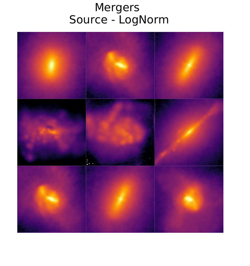

4 A. Ćiprijanović et al.
where || − 0 || is the Euclidean distance norm (where can be s between-class separability in the latent feature space, which makes
or t depending on the domain), and is the free parameter which the distinction between classes easier in the source domain. Fisher
determines the width of the kernel. loss produces a centroid for each class and effectively pushes la-
 Finally, we use MMD as our transfer loss: LTL,mmd = , effec- beled classes toward their respective centroids, thereby creating more
tively drawing the source and target distributions together in latent tightly clustered classes further apart from each other. It can be de-
space as the network aims to minimize the loss via backpropagation. fined as a function :
 LFL = (tr(Sw ), tr(Sb ))). (10)
2.1.2 Domain Adversarial Training ÍM Í m T
 Here, Sw = =1 =1 (h −c )(h −c ) captures the intra-
Domain adversarial training employs a Domain Adversarial Neural class dispersion of samples within each class, where h is the latent
Network (DANN) to distinguish between the source and target do- feature of the -th sample of the -th class (with M being the total
 number of classes). On the other hand, Sb = M T
 Í
mains (Ganin et al. 2016). DANNs are comprised of three parts: a =1 (c − c) (c − c)
feature extractor ( F ), label predictor ( L ), and domain classifier describes the distances of all class centroids c to the global center
 c= M 1 ÍM c . This global center, c, is meant to be optimized such
( D ). The first two parts can be found in any Convolutional Neural =1 
Network (CNN)— the feature extractor is built from convolutional that the centroids of the classes are pushed as far away as possible.
layers which extract features from images, while the label predictor Traces are used in the computation of the Fisher loss since they are
usually has fully-connected (dense) layers which output the class la- computationally efficient.
bel. The last part, the domain classifier, is unique to DANNs. It is To achieve the intended result of intra-class compactness and inter-
built from dense layers and optimized to predict the domain labels. class separability, Eq. 10 must be monotonically increasing with
This domain classifier is added after the feature extractor as a paral- respect to the trace of the intra-class matrix Sw and monotonically
lel branch to the label predictor. It includes a gradient reversal layer decreasing with respect to the trace of the inter-class matrix Sb . Thus,
which maximizes the loss for this branch of the neural network, thus as the loss is minimized via backpropagation, the distances within
achieving the adversarial objective of confusing the discriminator. classes will grow smaller and the distances between classes will
When the domain classifier fails to distinguish latent features from grow larger. There are two simple ways one can construct a Fisher
the two domains, the domain invariant features, i.e. the shared feature loss function obeying these constraints: Fisher trace ratio LFL =
space, is found. tr(Sw )/tr(Sb )) or Fisher trace difference LFL = tr(Sw ) − tr(Sb )). In
 Compared to regular CNNs which can learn the best features for this paper, we have chosen to use the Fisher trace ratio as our Fisher
classification, training DANNs can lead to a slight drop in classi- loss.
fication accuracy for the source domain because only the domain- As we mentioned in Eq. 2 for total loss, we can control the con-
invariant features are used. However, this will also lead to an increase tribution of all additional losses using the weight parameter . In the
in the classification accuracy in the new target domain which is our case of Fisher loss, we can separately weight the importance of the
objective. The total loss for a DANN is LDANN = Lclass − Ld , two matrices using w and b . Since we have chosen to use the trace
where Lclass is the loss for the image class label predictor L , while ratio Fisher loss LFL = w tr(Sw )/ b tr(Sb ), this gives FL = w / b .
Ld is the loss from the domain classifier D . Fine-tuning the trade-off
between these two quantities during the learning process is done with
 2.3 Entropy Minimization
the regularization parameter . Domain classifier loss is calculated
as: Fisher loss can only be used in the source domain since it requires
 1 ∑︁ 1 ∑︁ ground-truth labels to calculate intra-class centroids and the between
Ld = ( D ( F (xs )), s ) + ( D ( F (xt )), t ), class global center. However, Fisher loss can aid the discrimination
 s t
 xs ∈ Ds xt ∈ Dt between classes within the unlabeled target domain as well through
 (8) entropy minimization loss. Entropy minimization loss pushes exam-
 ples from the target domain toward source domain class centroids.
where ( D ( F (xs )), s ) and ( D ( F (xt )), t ) are the output Therefore, entropy minimization ensures better generalization of the
scores for the source domain and target domain labels, respectively. decision boundary between optimally discriminative and compact
Similarly to the class label predictor, the output scores for domain source domain classes to the target domain as well (Grandvalet &
labels are also calculated using cross-entropy loss on domain labels. Bengio 2005).
Finally, we can use domain classifier loss as our transfer loss: Entropy minimization loss is defined as:
LTL,adv = max{−Ld }. (9) M
 m ∑︁
 ∑︁
 LEM = − ( |h ) log ( |h ), (11)
 =1 =1
2.2 Fisher Loss
 where ( |h ) is the classifier output and the true label is not
The addition of Fisher loss to the classification and transfer losses needed. The above formula is based on Shannon’s entropy (Shannon
was demonstrated to further improve classification performance for 1948), which for a discrete probability distribution can be written as
source domain images in Zhang et al. (2020a). This improvement ( ) = − N
 Í
 =1 log2 .
in source classification can aid the performance of both MMD and
domain adversarial training transfer criteria. It is more generally
applicable than Scatter Component Analysis (Ghifary et al. 2017),
 3 NEURAL NETWORK ARCHITECTURES
which also results in class compactness, but can only be used in
conjunction with MMD and would not be practical for use with We present the performance of domain adaptation using the afore-
adversarial training methods (Zhang et al. 2020a). mentioned techniques in two neural networks— the simpler Deep-
 Minimizing Fisher loss leads to within-class compactness and Merge architecture with 174,626 trainable parameters (Ćiprijanović

MNRAS 000, 1–17 (2021)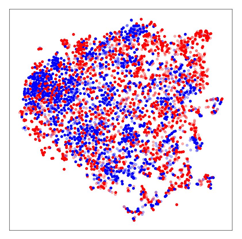

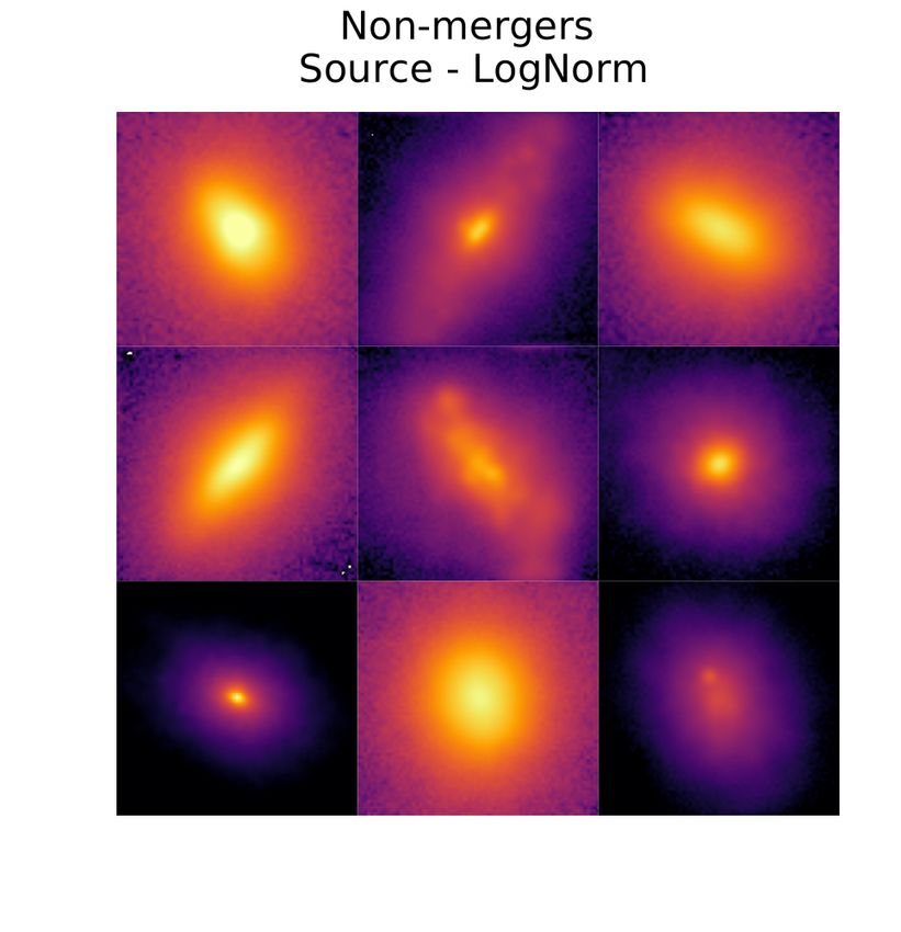
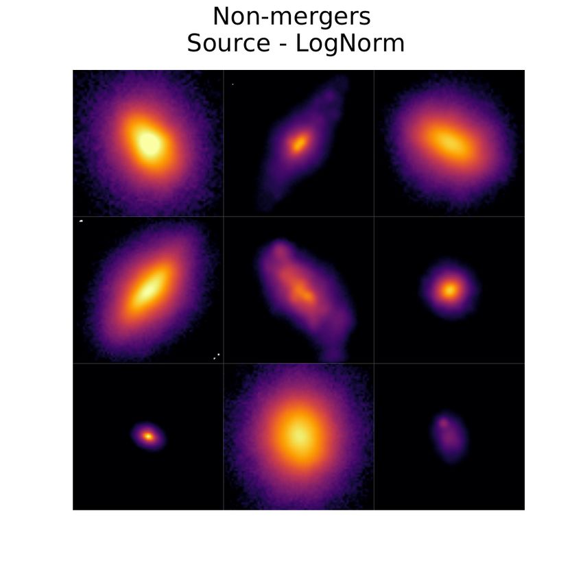
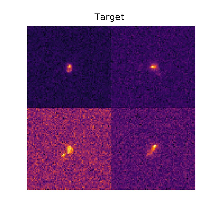
DeepMerge II: Building Robust Deep Learning Algorithms for Merging Galaxy Identification Across Domains 5
et al. 2020) and the more complex and well known network ResNet18
with 22,484,866 trainable parameters (He et al. 2015)— to compare
results across architectures. We decided to use the smallest standard
ResNet architecture, in order to more easily tackle possible overfitting
of the model, due to small sizes of merging galaxies datasets.
 The DeepMerge network, first introduced by Ćiprijanović et al.
(2020), is a simple CNN comprised of three convolutional layers
followed by batch normalization, max pooling, and dropout, and three
dense layers. In this paper, the dropout layers have been removed
such that the only regularization happens via L2 regularization of
the weight decay parameter in the optimizer. Additionally, the last
layer of the original DeepMerge network was updated to include
two neurons rather than one. For more details about the architecture
check Table A1 in the Appendix.
 ResNets were first proposed in the seminal paper He et al. (2015)
and have become one of the most widely-used network architectures
for image recognition. They are comprised of residual blocks; in the
case of ResNet18, blocks of two 3x3 convolutional layers are followed
by a ReLU nonlinearity. The chaining of these residual blocks enables
the network to retain high training accuracy performance even with
increasing network depth.
 The domain classifier used in adversarial domain training to cal-
culate transfer loss comprises of three dense layers, the first of which
is the same dimension of the extracted features in the base network
(either DeepMerge or ResNet18), such that these features form the
input into the domain classifier. The second layer has 1024 neurons,
followed by ReLU activation and dropout of 0.5, and the third has
one output neuron followed by Sigmoid activation, conveying the
domain chosen by the network.
 Details about training the networks can be found in Appendix A.
We also list all hyperparameters used for training in different exper-
iments in Table A2 and Table A3. Our parameter choice for each
experiment was informed by running hyperparameter searches using
DeepHyper (Balaprakash et al. 2018; Balaprakash et al. 2019). Figure 1. Galaxy images from Illustris-1 simulation at = 2. The left column
 shows merging galaxies and the right column shows non-mergers. The same
 objects are repeated across rows, with the top showing the source domain,
4 DATA the middle showing the target domain, and the bottom displaying the source
 objects with logarithmic color map normalization for enhanced visibility.
Here we present two dataset pairs for classifying distant merging
galaxies ( = 2) and nearby merging galaxies ( < 0.1).
 images are convolved with the PSF, with added random sky shot
 noise. This sky shot noise produces a 5 limiting surface brightness
4.1 Simulation-to-Simulation: Distant Merging Galaxies from of 25 magnitudes per square arc-second. More details about the
 Illustris dataset can be found in Ćiprijanović et al. (2020) and Snyder et al.
 (2019). The source and target domains contain 8120 mergers and
It is often very difficult to obtain real-sky observational data of la-
 7306 non-mergers, respectively. Each image is 75 × 75 pixels. We
beled mergers for deep learning models, especially at higher redshifts.
 divide these datasets into training, validation, and testing samples:
Therefore, both the source and target domain of our distant merging
 70% : 10% : 20%.
galaxy dataset are simulated.
 See Figure 1 for example images from this Illustris dataset: mergers
 We use the same dataset as in Ćiprijanović et al. (2020), where the
 are shown in the left column and non-mergers in the right column.
authors extract galaxies at redshift = 2 from Illustris-1 cosmologi-
 The top row shows images from the source domain, while the middle
cal simulation (Vogelsberger et al. 2014). The objects in this dataset
 row shows the target galaxies with the added noise. The bottom row
are labeled as mergers if they underwent a major merger (stellar mass
 shows the same group of top-row source images with logarithmic
ratios of 10 : 1) in a time window of 0.5 Gyr around when the Illus-
 color mapping in order to make the galaxies more visible to the
tris snapshot was taken. This means our merger sample includes both
 human eye.
past (happened before the snapshot) and future mergers (happened
after the snapshot). In Ćiprijanović et al. (2020), images contain two
filters, which mimic Hubble Space Telescope (HST) observations. In
 4.2 Simulation-to-Real: Nearby Merging Galaxies from
this paper we add a third (middle) filter to produce three filter HST
 Illustris and Real SDSS Images
images (ACS F814W, NC F356W, WFC3 F160W). This allows us to
use the images even with a more complex ResNet18 architecture. To test the ability of MMD and adversarial training in the astro-
 We produce two groups of images: source "pristine" images are nomical situations where they show the most promise— training on
convolved with a point-spread function (PSF); and target "noisy" simulated data with the prospect of applying the models to real data—

 MNRAS 000, 1–17 (2021)

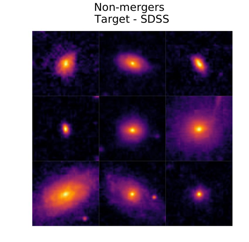
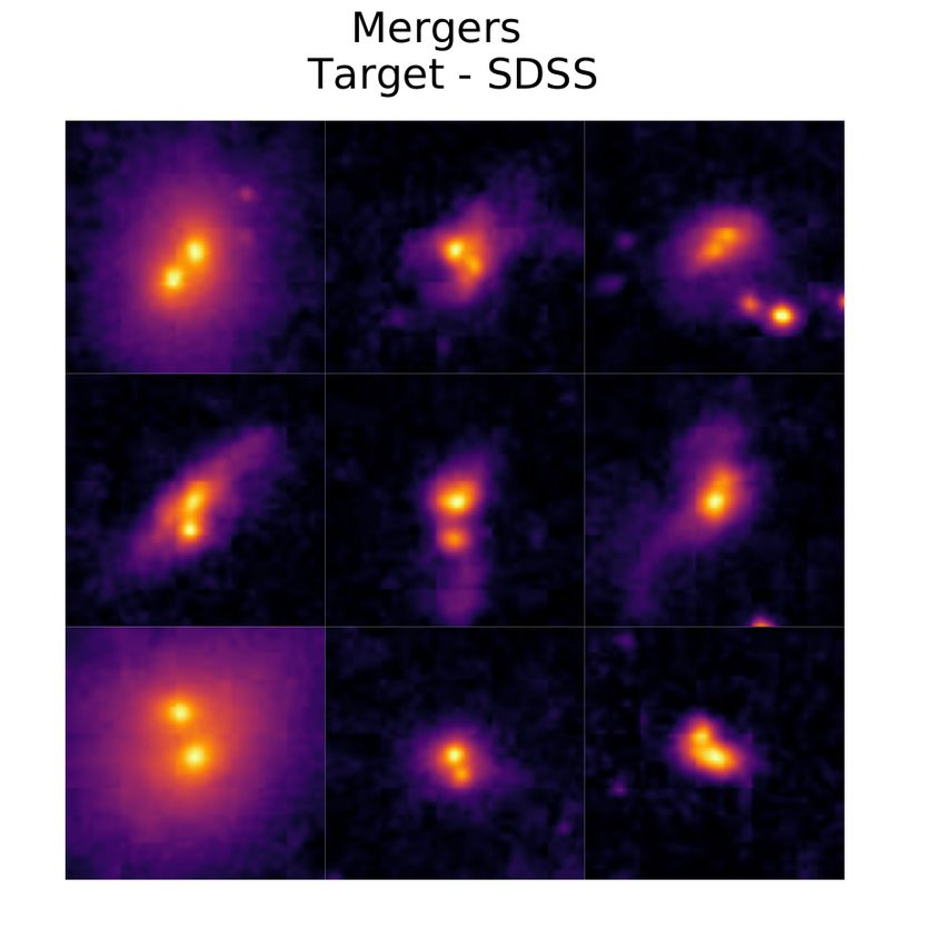
6 A. Ćiprijanović et al.
we need to use merging galaxies at lower redshifts where more real = 0 describes objects that are not merger-like and = 1
data is available. describes merger-like objects. Mergers included in Galaxy Zoo were
 also required to be between redshifts 0.005 < < 0.1.
 All available SDSS mergers also include a merger stage: separated
4.2.1 Source dataset: simulated images mergers (167 images), interacting (2523 images), post-mergers (310
 images). Since our source domain includes only post-mergers, we
In this scenario, attempting to make simulated images resemble real restrict our target dataset to only include the post-merger subclass
observations from a particular telescope is an important step for from SDSS. To obtain 3000 mergers, we augment the SDSS post-
domain adaptation techniques, since decreasing differences between merger images using the same techniques used in the source domain.
domains will make domain adaptation easier. Here our source data is To complete our target dataset, another 3000 non-merger galaxies in
comprised of simulated merging galaxies (major mergers) from the the 0.005 < < 0.1 redshift range were randomly selected from the
final snapshot at = 0 of Illustris-1, in a time window of 0.25 Gyr Galaxy Zoo project’s entire dataset by requiring < 0.2.
before the time the snapshot was taken. The fact that we use the
 We resize images from both domains to the same size as in
final snapshot of the simulation is an extremely important difference
 simulation-to-simulation example (75 × 75 pixels), and use the same
between this source domain dataset and the one described earlier: this
 split into training, validation and testing samples: 70% : 10% : 20%.
means that only past mergers (also called post-mergers) are included
 In Figure 2 we plot images from both domains. In the top row, we plot
instead of both past and future mergers. Since the simulation was
 post-mergers (left) and non-mergers (right) from Illustris simulation
stopped after this snapshot, images of future mergers that would
 at = 0, while in the bottom row we plot post-mergers (left) and
have merged during 0.25 Gyr after the snapshot are not available.
 non-mergers (right) from SDSS.
 This dataset was originally produced in Snyder et al. (2015). Here,
 Images from the target domain were visually classified, and most
images also include effects of dust implemented as a slab model
 of the target post-mergers clearly exhibit two bright galaxy cores,
based on the gas and metal density along the line of sight to each
 while images from the source domain display a greater variety of
pixel, similar to models by Nelson et al. (2018), De Lucia & Blaizot
 characteristics. Consequently, the two domains are extremely dis-
(2007), and Kitzbichler & White (2007). Images have three SDSS
 similar relative to the two domains in the simulation-to-simulation
filters ( , , ) and are also convolved with a Gaussian PSF (FWHM =
 example. The choices we detail above— using only post-mergers in
1 kpc) and re-binned to a constant pixel scale of 0.24 kpc. This scale
 both domains; including observational and dust effects and choosing
corresponds to 1 arcsec seeing for an object observed by SDSS at
 a small time window to avoid the inclusion of very relaxed merger
 = 0.05. Finally, random sky shot noise was added to these images
 systems in the source domain— were made in an attempt to make
by independently drawing from a Gaussian distribution for each pixel,
 the two domains as similar as possible. Still, the fact that the number
which produces average signal-to-noise ratio of 25.
 of individual mergers in both domains is very small, paired with the
 The simulated galaxies in this dataset contain a lower number of
 fact that their appearance can be quite different makes any domain
mergers compared to the = 2 snapshot used in our simulation-to-
 adaptation efforts quite challenging.
simulation experiments. Observational evidence shows that merger
rates today are much lower compared to the merger rate peak during
the "cosmic high noon" at ∼ 2 − 3 (Madau & Dickinson 2014),
which is where our galaxies from the previous example are located. 5 EXPERIMENTS
Our source domain dataset contains only 44 post-mergers and 5625
 CNNs outperform other machine learning methods for classification
non-mergers. We employ data augmentation in order to make a larger
 of merging galaxies (Snyder et al. 2019; Ćiprijanović et al. 2020).
source dataset, particularly focusing on mergers to make the classes
 However, in both Ćiprijanović et al. (2020) and Pearson et al. (2019),
balanced. We first augment mergers by using mirroring (vertical
 it was shown that, even though training and evaluating a CNN on
and horizontal), and rotation by 90◦ and 180◦ (which produces 220
 images from the same domain gives very good results, a simple model
images). Finally, these images are additionally augmented by random
 trained in one domain cannot perform classification in a different
angle rotation or zooming in/out. The final source dataset we use
 domain with high accuracy. To increase the performance of deep
contains 3000 : 3000 post-mergers and non-mergers (we truncate
 learning classifiers on a target dataset, we use the DA techniques
non-mergers to make the classes balanced).
 described in Section 2.
 We first train neural networks without the implementation of any
 DA techniques to determine the base performance for source and
4.2.2 Target dataset: observed images
 target images for each pair of datasets: simulated-to-simulated (Il-
Our target dataset is composed of observational SDSS images. We lustris = 2 with and without noise) and simulated-to-real (Illustris
follow dataset selection from Ackermann et al. (2018) and use the = 0 and SDSS). While we possess labels for both the source and
SDSS online image cutout server to get RGB (red, green, blue) target domain in both scenarios, this training is performed using la-
JPEG images of both merging and non-merging galaxies. These RGB beled source images exclusively. We only use the target image labels
images correspond to ( , , ) SDSS filters, as opposed to ( , , ) in in the testing phase to asses accuracy. We seek these performance
our source domain. We later align the order of filters in our source accuracies as the metric to improve upon through domain adaptation.
domain to correspond to this filter order. All of the galaxies selected We then run several domain adaptation experiments— using MMD
are from the Galaxy Zoo project (Lintott et al. 2008, 2010), which as transfer loss, adversarial training with DANN domain discrimi-
used crowd-sourcing to generate labels for 900,000 galaxies. We use nator loss as transfer loss, MMD as transfer loss with Fisher loss
the 3003 mergers identified in the Darg et al. (2010) catalogue; three and entropy minimization, and finally DANN adversarial training
of these mergers were unable to be retrieved due to faulty weblinks. with Fisher loss and entropy minimization— with both DeepMerge
This catalogue identified mergers through the weighted-merger-vote and ResNet18 architectures on the simulation-to-simulation dataset.
fraction, , which describes the confidence in the crowd-sourced Training with domain adaptation is performed using labeled source
label. Mergers were defined as galaxies with an > 0.4, where data and unlabeled target data. In the case of adversarial training, an

MNRAS 000, 1–17 (2021)

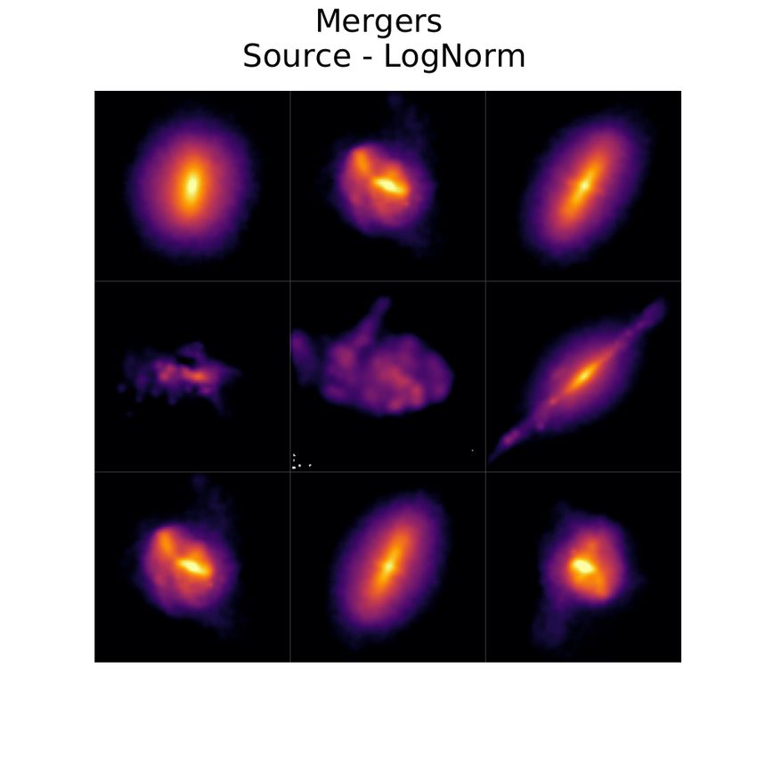
DeepMerge II: Building Robust Deep Learning Algorithms for Merging Galaxy Identification Across Domains 7
 6 RESULTS
 Throughout this paper we consider mergers the positive class (la-
 bel 1), and non-mergers the negative class (label 0). Consequently,
 correctly/incorrectly classified merger are true positives (TP)/false
 negatives (FN), while correctly/incorrectly classified non-mergers
 are true negatives (TN)/false positives (FP).
 We report classification accuracy, precision or purity: TP/(TP
 + FP), recall or completeness: TP/(TP + FN), and F1 score =
 2 Precision×Recall
 Precision+Recall . We also report the Area Under the Curve (AUC)
 score— the area under the Receiver Operating Characteristic (ROC)
 curve, which conveys the trade-off between true-positive rate and
 false-positive rate. Finally, we provide Brier score values, which
 measure the mean squared error between the predicted scores and
 the true labels; a perfect classifier would have a Brier score of zero.

 6.1 Simulation-to-Simulation Experiments
 Results of training the two classifiers without domain adaptation are
 given in the first row of Table 1. Training was performed on the
 source domain images, and test accuracy on source images is high
 for both networks in the base case without DA: 85% for DeepMerge
 and 81% for ResNet18. As was expected, without any domain adap-
 tation both classifiers are almost unable to classify target domain
Figure 2. Galaxy images from Illustris simulation at = 0 mimicking SDSS images; test accuracy for this domain are only 58% (DeepMerge)
observations (top row) and real SDSS images (bottom row). The left col- and 60% (ResNet18). Additionally, as expected, we noticed that the
umn shows post-merger galaxies, while the right column shows non-mergers.
 more complex ResNet18 was much more prone to overfitting ear-
Source domain images in the top row were plotted with a logarithmic color
map to make features more visible. Even when we select only post-mergers
 lier in the training than DeepMerge. We therefore implemented early
from SDSS we can still see that the merger class is different across the two stopping in our training in all experiments, as well as saving of the
domains. While the source domain contains more relaxed systems, the target best model before the training stops due to substantial overfitting.
contains galaxies near each other, with two bright clearly visible cores. We then trained DeepMerge and ResNet18 with both domain adap-
 tation techniques, each with and without Fisher loss and entropy
 minimization. Results from these DA experiments are also given in
 Table 1. We conclude that it is difficult to determine a single best
 technique across architectures. Additionally, inclusion of the Fisher
 loss and entropy minimization, implemented for within class com-
additional domain classifier branch is added to receive an input of pactness in both the source and target domains, does not always help.
features from base network. The parameters used for training both This might be due to the fact that multiple losses interact differ-
DeepMerge and ResNet18 for all simulation-to-simulation experi- ently depending on the network architecture and complexity of the
ments are given in the Appendix in Table A2. feature space. In short, simple hyperparameter grid searches, which
 Since larger networks are prone to overfitting, given the limited informed our parameter choices, are not a perfect solution to find
size of both source and target datasets in our simulation-to-real ex- the optimal hyperparameters for different experiments (a non-trivial
periments, we decided to only test it with the the smaller Deep- task that we leave for future studies). Despite our imperfect hyper-
Merge network. Similar to the experiments described above for the paramter choices, we assert that the results presented here convey
simulation-to-simulation dataset, we first train DeepMerge without an overall demonstration of the performance and improvements of
any domain adaptation in order to determine the base performance. domain adaptation techniques for cross-domain studies.
We then tried to improve target domain accuracy by training us- Next we take a closer look at experiments that were most success-
ing MMD and adversarial training, both with and without Fisher ful for DeepMerge and ResNet18. The best-performing DeepMerge
loss and entropy minimization. However, despite performing hyper- network experiments— MMD, adversarial training, and adversar-
parameter searches, domain adaptation was not successful, i.e. the ial training with Fisher loss and entropy minimization— reached
target domain accuracy was no better than random guessing. We then source domain accuracies of 87%. The accuracy in the target do-
turned our trials to combining MMD and adversarial training with main was largest with adversarial training at 79%, while with MMD
transfer learning from models successfully trained in simulation-to- it reached 77%. Consequently, the highest increase in target domain
simulation experiments. Hyperparameters used in training the model accuracy was 21% compared to the classifier without domain adapta-
in the simulation-to-real experiments are given in the Appendix in tion. Again, we assert that each experiment’s results could potentially
Table A3. be further improved with a different set of hyperparameters.
 To ensure reproducibility of our results prior to training, we fix the For ResNet18, we see a slightly smaller increase in target domain
random seeds used for image shuffling (before division into training, accuracies compared to improvements by DeepMerge. Because it is
validation and testing samples), as well as for random weight initial- a more complex network, it is harder to stop ResNet18 from learning
ization of our neural networks. The same images were used across more intricate details that are only found in the source domain. Target
experiments for training, as well as for testing afterwards to produce domain accuracies increase from 60% without domain adaptation to
the reported results. In Section 6 we report results for a fixed seed=1. 75% in the best performing experiment, which was MMD with ad-

 MNRAS 000, 1–17 (2021)

8 A. Ćiprijanović et al.

Table 1. Performance metrics of the DeepMerge and ResNet18 CNNs, on source and target domain test sets, without domain adaptation (first row) and when
domain adaptation techniques are used during training (all other rows). The table shows AUC, Accuracy, Precision, Recall, F1 score, and Brier score.
 Simulated-to-Simulated
 Source Target
 Loss Metric
 DeepMerge ResNet18 DeepMerge ResNet18
 AUC 0.92 0.88 0.74 0.73
 Accuracy 0.85 0.81 0.58 0.60
 No Domain Adaptation Precision 0.88 0.82 0.99 0.82
 Recall 0.83 0.83 0.08 0.31
 F1 score 0.86 0.83 0.14 0.45
 Brier score 0.11 0.14 0.47 0.23
 AUC 0.93 0.96 0.85 0.80
 Accuracy 0.87 0.90 0.77 0.74
 MMD Precision 0.88 0.93 0.81 0.75
 Recall 0.87 0.90 0.72 0.74
 F1 score 0.88 0.91 0.76 0.75
 Brier score 0.10 0.08 0.17 0.21
 AUC 0.92 0.94 0.86 0.81
 Accuracy 0.84 0.89 0.77 0.75
 MMD + Fisher + Entropy Precision 0.87 0.90 0.79 0.75
 Recall 0.84 0.90 0.75 0.78
 F1 score 0.86 0.86 0.77 0.77
 Brier score 0.11 0.09 0.16 0.19
 AUC 0.94 0.97 0.87 0.78
 Accuracy 0.87 0.92 0.79 0.72
 Adversarial Precision 0.88 0.93 0.79 0.74
 Recall 0.89 0.93 0.81 0.71
 F1 score 0.87 0.93 0.80 0.72
 Brier score 0.09 0.06 0.16 0.25
 AUC 0.94 0.94 0.82 0.75
 Accuracy 0.87 0.87 0.74 0.70
 Adv. + Fisher + Entropy Precision 0.90 0.92 0.78 0.83
 Recall 0.86 0.85 0.68 0.54
 F1 score 0.88 0.88 0.73 0.65
 Brier score 0.10 0.09 0.21 0.24

ditional Fisher loss and entropy minimization. and lines show values for the target domain while the dashed bars
 In experiments without DA, we allow the network to learn from all and lines show source domain performance.
available features that can be extracted rather than restricting to the See Appendix B for additional performance comparison between
set of domain-invariant features. It follows that, in training without training with and without domain adaptation for both networks on
DA, a perfectly optimized network should be able to reach its highest the simulation-to-simulation dataset.
source accuracy when not being forced to learn domain-invariant fea-
tures. In contrast to this expectation, we observe that the addition of
transfer and other losses slightly increases source domain accuracies 6.2 Simulation-to-Real Experiments
in almost all of the experiments we ran. We posit that this is first and
foremost the consequence of not finding the best set of hyperparame- We also evaluated the performance of these DA methods in the situ-
ters and that the additional transfer loss serves as a good regularizer, ation where the classifier is trained on simulated source domain im-
enabling longer training without overfitting. This is more prominent ages and tested on a target domain of observational telescope images.
in case of ResNet18, where source domain accuracies increase from Examples like this are much more complex than our simulation-to-
81% for no domain adaptation case to the highest value of 92% in simulation experiments due to the larger discrepancy between do-
the case of adversarial training. mains, as discussed at length in Subsection 4.2.
 For easier comparison, in Figure 3 we plot the performance val- Due to the perils of training a large network on such a small dataset,
ues from Table 1 for our test set of images. The top row of plots we decided to test domain adaptation techniques with only the smaller
shows results for the DeepMerge network, while the bottom row DeepMerge network. Without DA, DeepMerge reached an accuracy
is for ResNet18. Bar plots on the left show all performance met- of 92% in the source domain and 50% in the target domain in the
rics (accuracy, precision, recall, F1 score, Brier score, and AUC) testing phase. This was our baseline we try to improve upon in the
for our simulated-to-simulated experiments: no domain adaptation simulation-to-real DA experiments. Due to the extreme discrepancy
(navy blue), MMD (purple), MMD with Fisher and entropy mini- between domains, we also tested trained the DeepMerge network on
mization (dark purple), adversarial training (yellow), and adversarial the target domain directly, which resulted in an accuracy of 96% on
training with Fisher and entropy (pink). The two right panels show the target domain images. This is higher than for the source domain
ROC curves for all DeepMerge and ResNet18 experiments, with the of simulation images, confirming that the target domain is easier to
same color coding as in the bar plots. In all four panels, the solid bars train on since it is comprised of visually more apparent merging fea-
 tures.
 We then tried running hyperparameter grid searches with MMD

MNRAS 000, 1–17 (2021)

DeepMerge II: Building Robust Deep Learning Algorithms for Merging Galaxy Identification Across Domains 9
 DeepMerge

 ResNet18

Figure 3. The top panel shows classification results for DeepMerge network and the bottom panel for ResNet18. Left: Performance metrics for no domain
adaptation experiment (labeled "noDA") in navy blue, MMD in purple, MMD wih Fisher loss and entropy minimization (labeled "MMD+F") in dark purple,
adversarial training (labeled "ADA") in yellow and adversarial training with Fisher loss and entropy minimization (labeled "ADA+F") in pink. We plot values
for accuracy, precision, recall, F1 score, Brier score, and AUC. Dashed bars show results for the source domain and solid colored bars for the target domain.
Right: ROC curves with the same color and line style scheme. In the legend we also give AUC values for all five experiments.

and adversarial training, but were unable to successfully use do- on images of everyday objects from ImageNet (Deng et al. 2009).
main adaptation to improve target domain accuracies. This led us to They successfully trained the model on observed images of merging
conclude that problems with the size of our dataset, as well as the galaxies from SDSS and report classification precision, recall, and
difference between domains, was preventing the successful learning F1 score of 0.97, 0.96, 0.97. Similarly, in Wang et al. (2020), authors
of domain-invariant features. In the top row of Table 2, we report all use a VGG network (Simonyan & Zisserman 2015) pre-trained on
performance metrics for no domain adaptation case and in the mid- ImageNet to train on simulated images from the IllustrisTNG simu-
dle row we report results of using MMD only as transfer loss. Since lation at = 0.15 (Springel et al. 2018; Pillepich et al. 2018). They
no other method was successful, we omit reporting numbers for all report classification accuracy of 72% on simulated images, and then
other DA setups tested in the simulation-to-real experiments. Larger use the simulation-trained model to detect major mergers in KiDS (de
simulated training samples, more sophisticated domain adaptation Jong et al. 2013) and GAMA (Driver et al. 2009) observations.
methods that allow for better domain overlap of discrepant feature We decided to test if our simulated-to-real DA setup would benefit
distributions, or a combination of the two will advance the study of from transfer learning from a more similar dataset than ImageNet.
merging galaxies across the simulated-to-real domain in the future. Rather than proceeding with random weight initialization, we load
 the weights from our successfully trained DeepMerge networks in
 our simulated-to-simulated experiments. This way we can utilize ex-
6.2.1 Transfer Learning tracted features that relate to distant merging galaxies, which are
 much more similar to nearby merging galaxies, than features ex-
The approach we took to overcome our small dataset limitation was tracted from everyday objects.
to use transfer learning, where the weights from a neural network We tried training without freezing layers (allowing all weights in
pre-trained on different data are loaded before training the classifier the network to fine-tune to the new datasets), and freezing of con-
on the data of interest. volutional and batch normalization layers. The training performed
 Transfer learning has been used in previous studies of merging much better when all weights of the model were allowed to train
galaxies. For example, in Ackermann et al. (2018), authors use from their loaded checkpoint. This may be due to both the smaller
Xception (Chollet 2016), a large deep learning model, pre-trained

 MNRAS 000, 1–17 (2021)

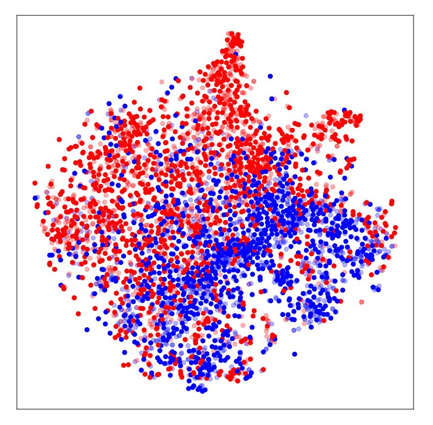
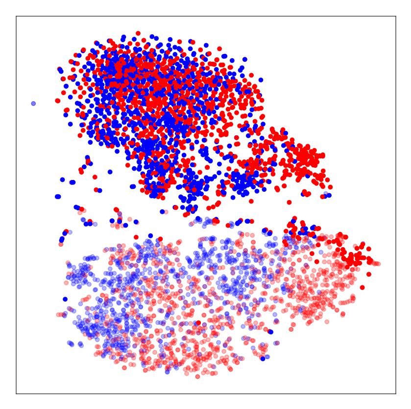
10 A. Ćiprijanović et al.

 DeepMerge

Figure 4. Left: Performance metrics for DeepMerge network for no domain adaptation experiment (labeled "noDA") in navy blue, MMD in purple, MMD with
transfer learning (labeled "MMD+TL") in yellow. We plot values for accuracy, precision, recall, F1 score, Brier score, and AUC. Dashed bars show results for
the source domain and solid colored bars for the target domain. Right: ROC curves with same color and line style scheme. In legend we also give AUC values
for all three experiments.

Table 2. Performance metrics of DeepMerge, on source simulated data and MMD and transfer learning. However, and most significantly, we
target observational data in the testing phase: without domain adaptation were able to achieve 69% in the target domain during the testing
(first row), MMD only (middle row), and MMD with tranfer learning (bottom phase of MMD with transfer learning— an increase of 19% com-
row). The table shows AUC, accuracy, precision, recall, F1 score, and Brier pared to noDA. In the bottom row of Table 2, we report performance
score. metrics for this transfer learning case.
 Simulated-to-Real For ease of comparison, we also plot performance metric values
 DeepMerge in the testing phase in Figure 4. Bar plots on the left show all perfor-
 Loss Metric
 Source Target mance metrics (accuracy, precision, recall, F1 score, Brier score, and
 AUC 0.97 0.58 AUC) for our simulated-to-real experiments— no domain adaptation
 Accuracy 0.92 0.50 (navy blue), MMD (purple), MMD with transfer learning (yellow).
 No Domain Adaptation Precision 0.91 0.50 ROC curves for these experiments are presented on the right, with
 Recall 0.92 0.80 the same color coding as in the bar plots. In both panels, the solid
 F1 score 0.92 0.62
 bars and lines show values for the target domain while the dashed
 Brier score 0.06 0.49
 bars and lines show source domain performance.
 AUC 0.98 0.60
 Accuracy 0.94 0.53 This experiment demonstrates that domain adaptation techniques
 MMD Precision 0.92 0.53 are very powerful. However, to be useful in a scientific context, we
 Recall 0.95 0.63 conclude that very careful data preprocessing to reduce domain dis-
 F1 score 0.94 0.58 crepancies and/or transfer learning to mitigate the problem of small
 Brier score 0.05 0.40 datasets is necessary. It is our hope that the introduction of these
 AUC 0.90 0.76 techniques to the astronomy community will spur innovation and
 Accuracy 0.83 0.69 encourage the use of more sophisticated DA methods that optimize
 Transfer Learning + MMD Precision 0.89 0.68 domain alignment for this sort of difficult astronomical tasks.
 Recall 0.74 0.74
 F1 score 0.80 0.71
 Brier score 0.13 0.23

 7 DISCUSSION
size of the DeepMerge network as well as the possible differences
in the appearance of galaxies in our experiments, with a particular We have demonstrated how MMD and domain adversarial train-
emphasis on the very different appearance of real SDSS mergers ing substantially increase the performance of simulated-to-simulated
compared to simulated ones. This probably led to the necessity of learning in the context of galaxy merger classification. For Deep-
the network finding better-suited domain invariant features when real Merge, the average accuracy benefit of these techniques was 18.75%
data is included, which can be more easily found when convolutional in the target domain; for ResNet18, the average benefit was 12.75%.
layers are allowed to train. While unable to show positive results with adversarial domain adap-
 We also performed a hyperparameter search for both MMD and tation training on our simulated-to-real dataset, pairing MMD with
adversarial domain adaptation with transfer learning, and were able transfer learning achieved a substantial increase in target domain ac-
to find a configuration for successful DA with MMD. Since the do- curacy of 19% with DeepMerge.
main discrepancy in the case of simulated-to-real images was large, We believe that both techniques show great promise for use in
successfully learning common features led to the reduction of source astronomy. Here we discuss their interpretability with the aid of t-
domain accuracy from 92% without domain adaptation to 83% with Distributed Stochastic Neighbor Embeddings (t-SNEs) and Gradient-

MNRAS 000, 1–17 (2021)

DeepMerge II: Building Robust Deep Learning Algorithms for Merging Galaxy Identification Across Domains 11
Class Activation Mappings (Grad-CAMs); and provide an outlook which differently trained models identify as the most salient informa-
on their potential for use within the scientific community. tion in the image. This method calculates class -specific gradients
 
 of the output score with respect to the activation maps
 
7.1 Model Interpretability: Understanding the Extracted (i.e. feature maps) of the last convolutional layer in the network.
 Features with t-SNEs Here activation map dimensions are × = pixels and lists the
 number of feature maps. These gradients are global-average-pooled
To better understand the effect of domain adaptation, we visu- to calculate the importance weights for a particular class :
alize the distribution of the extracted features with t-Distributed
Stochastic Neighbor Embeddings (t-SNE) plots by projecting the 1 ∑︁ ∑︁ 
 = . (12)
high-dimensional feature space to a more familiar two-dimensional 
 
plane (van der Maaten & Hinton 2008). This method calculates the
probability distribution over data point pairs, assigning a higher prob- Grad-CAMs are then produced by applying a ReLU function (to
ability to similar objects and a lower probability to dissimilar pairs, extract positive activation regions for the particular class ) to the
in both the latent feature space and in the two-dimensional mapping. weighted combination of feature maps in the last convolutional
By minimizing the Kullback–Leibler (KL) divergence (Kullback & layer:
Leibler 1951) between the two distributions, the t-SNE method en- ∑︁
 !
sures the similarity between the actual distribution and the projection. Grad−CAM, = ReLU 
 . (13)
Despite its usefulness, we emphasize that t-SNE is a non-linear algo- 
rithm and adapts to data by performing different transformations in
 In Figure 6, we plot the last convolutional layer Grad-CAMs for
each region. This can lead to clumps with highly-concentrated points
 simulation-to-simulation experiments with the DeepMerge network.
appearing as very large groups, i.e. it is difficult to compare relative
 We display plots for DeepMerge instead of ResNet18 due to the
sizes of clusters in t-SNE plot renderings. Additionally, the outputted
 fact that the dimension of the last convolutional layer in ResNet18 is
two-dimensional embeddings are entirely dependent on several user-
 smaller, resulting in low-resolution Grad-CAMs that are much harder
defined parameters. For more details on t-SNE best practices, see
 to interpret. The first column shows an example of a merging galaxy
Wattenberg et al. (2016).
 from the source domain at the top and from the target domain at the
 We implemented an option to plot t-SNEs in our training method
 bottom; recall that these two domains differ only by the inclusion of
to demonstrate the changes in extracted features from the source and
 noise. The second, third, and fourth columns show Grad-CAMs for
target domain across a series of epochs. In Figure 5 we plot t-SNE
 the images in question for classification into a merger class, when
plots for DeepMerge before the start of the training in the first panel,
 training without DA, with MMD, and with MMD, Fisher loss, and
and t-SNE plots after some training— when no domain adaptation
 entropy minimization, respectively.
is implemented in the second panel, when MMD as transfer loss is
 In the case of training without domain adaptation in the second
used in the third panel, when MMD with Fisher loss and entropy
 column, the network is focusing on the periphery of the galaxy in
minimization is used in the fourth panel. We confirm that domain ad-
 the source domain, exactly where a lot of interesting asymmetric and
versarial training t-SNEs are virtually indistinguishable from MMD
 clumpy features are expected to appear in the case of mergers. These
plots, so we omit the repeat here. On all t-SNE plots, red and blue
 features are faint, and a lot of this information is lost in the target
colored dots represent the two classes— mergers and non-mergers,
 domain due to the inclusion of mimicked observational noise. As ex-
respectively— and transparent dots represent the source domain,
 pected, the classifier does not work in the target domain: we can see
while opaque dots represent the target domain.
 that the network focuses on the noise instead. When domain adapta-
 Before the start of training, classes are completely mixed together
 tion is introduced— MMD in the third row and MMD with Fisher
and domains are separated (first panel). With no domain adaptation,
 loss and entropy minimization in the fourth column— the network
we see that even after some training, domains remain separated (sec-
 learns to focus on the central brightest regions of the galaxy, which
ond panel). With domain adaptation but no Fisher loss or entropy
 are visible in both domains, and successfully performs classification
minimization (third panel), we see that features from both domains
 in both cases.
completely overlap. We can see that both classes exhibit some clump-
 Likewise, we plot Grad-CAMs for the simulated-to-real exper-
ing but the structure of both classes is quite complex. Finally, in the
 iments with the DeepMerge network in Figure 7. Here we show
fourth panel, we also include Fisher loss and entropy minimization
 multiple true merger images from the source and target domains in
which helps the two classes separate more in both domains.
 the top left and right columns, respectively. The second and third
 row show Grad-CAMs for these images when training without do-
 main adaptation to highlight what the network focuses on for both
7.2 Model Interpretability: Visualizing Salient Regions in
 merger and non-merger classes. Finally, the fourth and fifth rows
 Input Images with Grad-CAMs
 show merger class and non-merger class Grad-CAMs for training
Another way of probing deep neural network models is by identi- with MMD with transfer learning.
fying regions in the input images that proved most important for In the source domain Grad-CAMs— where the classifier works
classification as a particular class. Domain adaptation should lead to with and without domain adaptation— the neural network searches
differences in these important regions. In particular, without domain the periphery when classifying an example as a merger, while it fo-
adaptation, the neural network can often identify incorrect or spu- cuses at the bright center when classifying non-mergers. This is to be
rious regions in images it was not trained on in the target domain, expected, since mergers often have a lot of useful information on the
while the classifier that works correctly should focus on regions that periphery, while non-mergers are often very compact and only have
contain useful information for the given classification task. a bright center in the middle of the image. On the other hand, the
 Here we will use the Gradient-weighted Class Activation Mapping Grad-CAMs for the target domain without domain adaptation, i.e. for
(Grad-CAM) method (Selvaraju et al. 2020) to visualize the regions the unsuccessful classifier, demonstrate the network’s focus on the

 MNRAS 000, 1–17 (2021)