The education chasing labor rush in China identified by a heterogeneous migration network game - Nature
←
→
Page content transcription
If your browser does not render page correctly, please read the page content below
www.nature.com/scientificreports
OPEN The education‑chasing labor
rush in China identified
by a heterogeneous
migration‑network game
Xiaoqi Zhang1,7, Yanqiao Zheng2,7*, Zhijun Zhao3, Xinyue Ye4, Peng Zhang3, Yougui Wang5 &
Zhan Chen6
Despite persistent efforts in understanding the motives and patterns of human migration behaviors,
little is known about the microscopic mechanism that drives migration and its association with
migrant types. To fill the gap, we develop a population game model in which migrants are allowed
to be heterogeneous and decide interactively on their destination, the resulting migration network
emerges naturally as an Nash equilibrium and depends continuously on migrant features. We apply
the model to Chinese labor migration data at the current and expected stages, aiming to quantify
migration behavior and decision mode for different migrant groups and at different stages. We find
the type-specific migration network differs significantly for migrants with different age, income
and education level, and also differs from the aggregated network at both stages. However, a
deep analysis on model performance suggests a different picture, stability exists for the decision
mechanism behind the “as-if” unstable migration behavior, which also explains the relative
invariance of low migration efficiency in different settings. Finally, by a classification of cities from the
estimated game, we find the richness of education resources is the most critical determinant of city
attractiveness for migrants, which gives hint to city managers in migration policy design.
Uncovering the mechanisms that govern the inter-regional migration behavior of human beings is critical for
understanding and managing a wide range of issues that interest both social scientists and policy makers, from
analyzing the motives and welfare change of migrants to the design of migration p olicies1–8. The increased
availability of large migration data sets that capture details of migration activities creates an unprecedented
opportunity to explore the motivations, consequences and patterns of migration. The early works in this field
aim at identifying the overall network patterns provided the occurrence of migration1,9–11, modelling the human
interaction dynamics that drive migration to happen1,12–22, and quantifying the casual relationship between
various social-economic factors and migration d ecision1–6,23–27. Apart from those topics, there is a recent wave
of studies focusing on unifying the migration decision-making, human interactions and the migration pattern
recognition together, so as to better understand the complexity of migration. It has been shown that the classical
estinations12–21 can be derived from a destination choice model (DCM)
gravity law of migration across multiple d
for a variety of migrants coming from different starting locations. A more recent work28 shows that interactions
among migrants can be added into the DCM framework, by which the DCM becomes the destination choice
game (DCG) that include DCM as a special case . The so-called “route congestion” e ffect11,28–30 can be formally
studied within the DCG framework, which merges the heterogeneity of migrants on their starting locations and
their interactions together, helping DCG generate better fitting to the observed migration trend.
1
National School of Development, Southeast University, Nanjing 210000, China. 2School of Finance, Zhejiang
University of Finance and Economics, Hangzhou 310018, China. 3Institute of Economics, Chinese Academy of
Social Science, Beijing 100836, China. 4Department of Landscape Architecture and Urban Planning, Texas A&M
University, College Station, TX 77840, USA. 5School of Systems Science, Beijing Normal University, Beijing 100875,
China. 6School of Statistics, Capital University of Economics and Business, Beijing 100070, China. 7These authors
contributed equally: Xiaoqi Zhang and Yanqiao Zheng. *email: zhengyanqiao@hotmail.com
Scientific Reports | (2020) 10:12917 | https://doi.org/10.1038/s41598-020-68913-3 1
Vol.:(0123456789)www.nature.com/scientificreports/
In addition to the heterogeneity for the starting locations and the interactions among migrants, the other
fundamental driving force of migration is the benefits that migration can bring to migrants. The benefits of
migration could depend on a variety of migrant-level social-economic factors in a complex w ay1–6,23–27. Econo-
mists and sociologists have made persistent effort in both qualitatively and quantitatively understanding the
relationship between migration decision and the social-economic factors, such as the education, age, income,
family wealth, gender difference and social c apital1,3,4,27,31–34. It is shown that migration is profitable for young and
poor migrants as it grants them and their later generations with the chance to chase well-paid job opportunity,
better education and/or healthcare s ervices8,31,35–37. On the ohter hand, migration is costly and hard to afford for
the migrants with limited family wealth, low education level and lacking of social connection in the potential
destinations3,4,33,38–40. Therefore, migration is essentially the consequence of a trade off between the benefit and
cost, the social-economic factors are important as they shape the way to calculate the benefit and cost for differ-
ent types of migrant. On that basis, a natural question is arisen, which factor is most influential for migration
decision, is migration for chasing better education, healthcare services, job opportunity and/or the others? The
other related question is whether the relationship between the social-economic factors and migration decisions
can change over time or is stationary for a long period. This question is critical for multi-stage migrations, but
due to the limitation in both the data and the empirical methodology, it is rarely studied in the literature. It turns
out that including the migrant-level social-economic features into the migration decision process is indispensa-
ble for answering above questions, but by now only the location-level heterogeneity are formally studied in the
framework of DCM/DCG, the variation of the migrant-level features has not yet been included. So, we ask: how
to incorporate the migrant-level social-economic features into the DCM/DCG framework to study the migra-
tion behavior? Can the inclusion of migrant-level features help generate better forecast for the real destination
selection? Will they give hint to the deep motives of inter-regional migration behavior and its dynamics?
It is not trivial to extend the location-level heterogeneity to the migrant-level heterogeneity in the DCG framework.
So, in order to address above questions, we propose a population game to model the interactive migration decision in
which the migrant-level features are added through a continuum feature space. With the help of adding migrant-level
features, many meaningful mechanisms, other than the classical congestion effect, route congestion effect and the
migration cost e ffect28,39, can be well represented in our model, such as the “subjective congestion effect”, capturing
the interpersonal difference in evaluating the congestion and its dependence on migrant types. To our best knowledge,
these mechanisms have not yet been formally studied in the existing literature within the context of migration, despite
their usefulness in classifying and identifying the attractiveness of destinations, measuring migration efficiency and so
forth. Our new model is fittable by real data through a mild modification of the game-econometric technique41–45. The
numeric analysis of the model is based on a resume data set extracted from one most famous online job platform in
China. The data supports the analysis of two-stage migrations, by which some dynamic facets of the migration pattern
can be studied. We identify and compare the two-stage labor migration networks, the forecast accuracy and migration
(in)efficiency are also analyzed as by-products of the model, which grant us the chance to identify the stationary nature
of the migration decision pattern over time. Finally, we highlight that although the analysis in this paper is mainly
based on Chinese labor migration data, our method is general and not restricted to labor force migration in China, it
can be applied to analyzing human migration behavior in a wide range of settings, such as the patient transfer behavior
among hospitals, international immigration behavior and the vehicle route selection issues.
The remaining sections of the paper is organized as the following. In the result section, an brief overview and
visualization to the migration dataset studied in the paper are provided, followed by a formal description on
the migration game model and the equilibria migration network, inefficiency index network derived from the
model. On the basis of model fitting, we discuss the stationary nature of the hidden migration decision pattern
behind the two-stage migration, and sketch how the migrant-level heterogeneity affects the migration patterns
and the migration efficiency. In the end, we introduce a classification criterion for cities according to the inef-
ficiency level of migration flows and briefly discuss the implication of applying the classification to our data. In
discussion section, we discuss the further implication of our game model and data analysis. "Method" section
introduces the technical details of the set-up of migration game model and its training procedure.
Results
Data description and the network structure of aggregated migration flows. We study the labor
force migration of Chinese online job-seekers by a large resume dataset. The resume data is collected from Zhao-
pin.com that is one leading online platform for job seeking in China and has a resume database consisting of
tens of million resumes filled by real job-seekers when they registered on this platform. Since the filled resumes
have high probability to be viewed by HRs from the intended recruiters, the information filled by job-seekers is
believed to reflect their truth and is updated in time. The questions mandatory to be answered include the gen-
der, age, marriage status, education experience, past working experience (most job seekers on zhaopin.com has
at least one job before), the previous working industries and so on, from which 77 migrant-level feature variables
can be extracted (a complete statistic description of these variables in our sample can be found in the supplemen-
tary to the paper). The resume also contains the information of migrant’s hukou place, the current working place,
the expected working places. Since the hukou place of job seekers can be identified as the place where they come
from, the resume data set provides a two-stage OD trajectory data set for the labor force migration in China that
are the stage (1): hukou place → current working place and stage (2): current → expected working place.
The data that we have the access is a purely random subsample of the full resume database which consists of
resumes from 80,000 job-seekers (after dropping the records with missing values, 75,616 records are remained),
the most recent update time of the resumes in this sample is by Jun. 2017. The included hukou places, working
places and expected working places cover 400+ cities in China which include all the 286 prefecture-level cities
and a set of lower-level cities of China, therefore we believe the subsample presents a good representative for the
Scientific Reports | (2020) 10:12917 | https://doi.org/10.1038/s41598-020-68913-3 2
Vol:.(1234567890)www.nature.com/scientificreports/
Figure 1. Overall migration network for the two-stage migrations (a,b) sketch the aggregated migration network
formed by the mean conditional migration probability from the origin city (group) to the destination city (group).
To simplify network structure, only the 178 cities included in the officially declared 21 major city clusters are
plotted with their exact geographic locations (longitude v.s. latitude). All the cities out of the 21 city clusters are
clapsed into one point labeled with “other cities”, the location of this point does not have any geographic sense
and only the arrows linking this point with the others are meaningful. The central cities in the 21 city clusters are
highlighted with their name labeled. The bold arrows between city pairs always point toward the destination city,
the size, darkness and opacity of the arrow represent the value of the aggregated mean migration probability. For
the simplicity of representation, the aggregated mean migration probability is calculated only for central cities of
the 21 city clusters and the “other cities” through summing up the mean migration probability between all city
pairs in the origin and destination city clusters, therefore all bold arrows are always link two central cities (or the
“other cities”). The migration flows within each of the 21 city clusters are kept and represented as the slim arrows,
their size, darkness and opacity represent the absolute value of the migration probability from the origin to the
destination. (c,d) present the to-degree of every city cluster from the other city clusters and the total link weight
within every city cluster (the sum of migration probabilities between all city pairs within a city cluster) for the
migration network of stage (1) and (2), respectively. The to-degree reflect the attractiveness of a city cluster and
the total link weight charaterize the tightness of inner-connection within each of the city clusters.
city-level labor force migration trend at least for the sub-population who seek job online. To avoid over-fitting,
we group all the destination cities into 22 city clusters among which the first 21 city clusters are officially declared
in the Chinese Statistical Yearbook (2015), the last one consists the cities that are not contained in any of the
officially declared city clusters.
From the data, the aggregated migration network for the two stages can be calculated simply by counting the
number of sampled migrants who migrate between every city pair. We can discuss the structural features of the
migration network and its structural changes for the two migration stages. The two-stage networks are presented
in Fig. 1a,b, where to generate clean plots, we only display the migration arrows across the 22 city clusters and the
migration arrows within every city cluster. Comparing the two plots, the decentralization or multi-centralization
trend is observed, and this trend can also be verified through comparing Fig. 1c,d where the blue line represents
the total to-degree of every city cluster. From Fig. 1a,c, during the first stage, Beijing is the unique global flow-
in center of all migrants, attracting migrants from both the other major cities (city clusters) in China, such as
Shanghai, Guangzhou, and the lower-level periphery cities (grouped within “Other cities”). Although there do
exist a couple of local flow-in centers such as Changchun in the north China and Shanghai in the East China,
while their attractiveness is not comparable to Beijing at all. In contrast, during stage (2), multiple global flow-
in centers emerge and they are detectible from comparing Fig. 1b,d. The local centers, such as Guangzhou,
Zhengzhou and Xi’an, are upgrade to global centers and their attractiveness becomes in line with Beijing, which
impedes the leading position of Beijing. The attractiveness of Beijing is even reduced in the absolute sense that
the strong migration flows from the local centers, such as Shanghai, Fuzhou, Guangzhou and Shenyang, in stage
(2), are significantly weakened or even disappears during stage (2). Finally, during stage (2), many tier-2 cities,
such as Zhengzhou, Changsha and Xi’an, starts to be attractive for migrants who come from periphery cities. If
we focus on the within-cluster migration trend, the difference between the stage (1) and (2) migration is also
Scientific Reports | (2020) 10:12917 | https://doi.org/10.1038/s41598-020-68913-3 3
Vol.:(0123456789)www.nature.com/scientificreports/
remarkable and coincides with the trend of decentralization. In fact, by the comparison between Fig. 1c,d, the
internal migration intensity is strengthened significantly for two city clusters in the stage (2) that are the set
of other cities and city cluster centered at Beijing. The former implies an increasing trend of the out-of-center
migration46, while the later implies the decline of Beijing in terms of absorbing local migrants which reinforces
the finding that the attractiveness of Beijing is reduced in the absolute sense.
The observed decentralization trend is highly consistent with the divergence in city development planning
and migrant-related policies since 2016 between the capital city Beijing and the other major cities in the middle
and western area of China. Since 2016, Beijing started to control its population scale, issue unfriendly residential
policies that expel the so-called “low-end” migrants who are the low-educated, low-skilled, low-income and
elderly contractor workers without registration in local hukou system. In the mean time, many tier-2 cities in the
middle and western area of China, such as Xi’an, Chongqing, Chengdu, Wuhan, and cities in the Yangtze river
delta area, such as Hangzhou and Nanjing, and cities in the Pearl river delta area, such as Shenzhen and Guang-
zhou, became migrant-friendly and relaxed the hukou restriction to attract young migrants with relatively high
education level. Since the second-stage migration in our dataset only refers to the expected migration which has
not yet happened in reality, the expectation of migrant workers reacts much more quickly to the policy change
than their real migration decision, the structural change of the migration network between the two stages is by
and large attributable to the non-homogeneous change of migration policy in different cities.
Although the overall migration network is informative, it is not complete. In reality, the migration network
often varies along with migrant types, such as the education, income and a ge3,34,38,47, while the aggregated net-
work fails to detect the difference. In addition, there are complicated interactions among migrants which also
contribute to the formation of migration network28 but are not reflected in the aggregated network. To this end,
we shall develop an empirically-fittible population game model for further investigation.
A family of large migration game. For simplicity we focus on the origin-destination (OD) type of migra-
tion trajectories, but the framework can be easily extended to more general situations. To formulate the interac-
tions among migrants, a large population game is established where the player set is viewed as a large random
sample drawn from a continuum feature space and all the strategies that players can select are identified as the
set of destination locations. The continuum feature space assumption is designed to capture the heterogeneity of
players and the fact that there are always enormous players involved in the migration analysis. For short, we shall
call this game model as migration game throughout the paper.
Formally, consider a family of normal-form games defined through the following four components and
represented as the tuple G(XN ⊂ P := C × Rp , C, µ, U):
A1. Pure strategies: denote C = {c1 , . . . , cn } as the pure strategy set which consists of all possible destination
locations for players.
A2. Players: denote Rp as the p-dimensional feature space, every x ∈ Rp represents a personal feature profile
that associates with a given player (type). Augmenting Rp with the origin place C forms the full set of
potential players characterized by both their personal and location features, denoted as P = C × Rp .
The set of N players XN is randomly drawn from P, according to a known distribution µ, which can be
interpreted as the population distribution.
A3. Mixed strategy: players are allowed to take mixed strategy, the mixed strategy set is represented as the set of
|C|−1
vector-valued function P = {P : XN → SC } where SC = {(p0 , . . . , p|C|−1 ) ∈ Rc : pi ≥ 0, i=0 pi = 1}
is the |C| − 1 dimensional simplex, |C| is the cardinality of C . Then, for every destination j ∈ C , the jth
coordinate projection Pj (i, x) will be the probability that a player (i, x) ∈ XN selects to migrate to j under
the mixed strategy P. Without loss of generality, we assume P ∈ P is smooth up to a certain order with
respect to x ∈ P, i.e. P is the restriction of a smooth function onto XN , which implies that two players
who are similar to each other in both of origin and features should make similar choice of strategies to
some extent.
A4. Utility: denote up as the pure strategy utility function of players, it takes the following form for a given
player x+ = (i, x) ∈ XN and a pure strategy profile s = {sx+′ ∈ C : x+ ′ ∈ X }:
N
1 �
′
up (x+ , j, s−x+ ) = F (1)
� �
I(sx+′ = j)T(x+ , x+ ) − g x+ , j
N −1 ′
x + � =x +
where s−x+ is a pure strategy combination executed by players other than the decision player x+, I is the indica-
tor function. F is a continuous function; T is a pairing weight function valued in the unit interval [0, 1] which,
for a given player x+, describes which group of competitors, namely {x+ ′ ∈ X : T(x , x ′ ) > 0}, will be taken
N + +
into account and how influential, measured by the value of function T(x+ , ·), the competitors are for x+; g is
interpreted as the ideal population ratio that the destination location should have, which is a kind of private
information for every player and the features of every player can affect this quantity in a certain way. The util-
ity for mixed strategy is calculated from Eq. (1) by the standard von-Neumann–Morgenstern expected utility
theory, denoted as UvNM .
For every pure strategy j, Eq. (1) postulates that the utility it brings for every decision player depends on the
difference between the actual population ratio [represented as the partial sum term in Eq. (1)] and the ideal
population ratio [represented as the value of function g in Eq. (1)]. This difference can be interpreted as a measure
for the degree of congestion in the destination city. As both the ways to count the actual population ratio and
the ideal population ratio in Eq. (1) are allowed to vary from player to player, the congestion effect studied in
Scientific Reports | (2020) 10:12917 | https://doi.org/10.1038/s41598-020-68913-3 4
Vol:.(1234567890)www.nature.com/scientificreports/
this paper is essentially the subjective congestion effect, which gives full respect to the migrant-level heteroge-
neity, and is more flexible, including the widely studied congestion effect and the route congestion e ffect11,28–30
as special cases. For the actual population ratio of a given decision player, only those players within the target
group are counted, while which player is in the target group is completely determined by the pairing function
T(x+ , ·) evaluated at the feature type of the decision player. Hence, the pairing function T encodes the relationship
among players, it can be interpreted as the continuous-version adjacency matrix of a player-to-player network.
This player-to-player network is closely related to the concept of “social capital” in the studies of social network,
including it into the utility function helps establish a quantitative connection between the adjacency matrix
of the social network among migrants and that of the migration network among r egions22. This connection is
important to understand the formation of migration trajectories. To our best knowledge, our work is the first
attempt to connect the two networks together at the adjacency-matrix level.
The ideal population ratio is also conditional on the feature of every player. This is because different players
often disagree with each other, the disagreement can come from both the difference in personal characteristics
(represented through their feature vector x) and the different original c ities1,28. For instance, local residents with
higher education level are more likely to survive in expensive meta-cities than those migrants with lower edu-
cation level, consequently, the former group of people tend to evaluate a greater g for big cities, while the later
group would assign a greater g to small and cheap cities when all others equal.
Throughout the application of the current paper, we simply assume F(x) = −x 2 , and g is parametrized
through the logistic form
1
g(i, x, j|θg ) = ⊤ · x − θ⊤ · x − θ⊤ · x )
, (2)
1 + exp(−θg,1 i g,2 g,3 j
where x is the person-level feature vector for a given player, xi and xj are the city-level feature vectors associated
with the origin city i and destination city j, respectively. θg (:= (θg,1 , θg,2 , θg,3 )) consists of the three coefficient
vectors associated with the feature xi , x and xj . Under this specification, we assume that every job-seeker obtain
utility from migration to city j through comparing the difference between his/her subjective optimal population
ratio of city j measured by g(i, x, j) and the actual ratio of job seekers that select to migrate into j. Using quadratic
functional form for F(x) captures that the utility is maximized if and only if the actual population ratio is just the
ideal ratio, both overwhelming and unsaturatedness would lower down the attractiveness of a destination (notice
that the quadratic form of F can be generalized to any functional form preserving the preference order that would
have no impact on the current analytic and numerical results, for instance the quadratic form can be replaced
by another function that has unique peak value and is symmetric with respect to the peak). This specification
captures the dynamics of migration in many real world settings (e.g. the labor force migration game, the vehicle
route selection game), similar utility functions are also used in the l iterature39.
For the pairing function and T, we consider two
alternatives that are the constant function T ≡ 1 and the
binary({0, 1})-valued function with T (i, x), (i′ , x ′ ) = 1 if and only if i = i′ . The later option describes the peer
effect behind migration by which migrants only take their “peers”, the migrants who come from the same ori-
gin, into account. A preliminary analysis shows that the constant function dominates the “peer-effect” pairing
function in forecast accuracy for migration decision at both migration stages, therefore, we would only focus on
the simpler setting T ≡ 1 in the following sections. One reason for the relative disadvantage of the peer-effect T
might be that the destination locations in our data are the city-level locations which are too-large to allow the
peer effect to work.
Finally, note that under the adjacency matrix interpretation of T, the constant pairing T ≡ 1 is equivalent to
that the social network that drive the formation of migration network is essentially a fully-connected network.
In the other words, every job-seeker in the game will put equal weight to the decision of all the other players.
This assumption is a bit weird as in reality job seekers is not possible to know all their competitors. But on the
other hand, this assumption is equivalent to ask the job-seekers read the officially published population data of
every city, which is not that unrealistic any more. It is definitely possible to set a more subtle form of the pairing
function T so as to better reflect the impact of social networks among job seekers, but that is beyond the scope
of both the data and the current study, we leave it for future studies.
Equilibrium, migration network and efficiency. The actual migration should happen in the way that every
migrant in the system can only move to the destination that maximizes their utility given the choice of the oth-
ers, which can be perfectly captured by the Nash equilibrium of the migration game. In fact, we can assume the
following without loss of generality.
Assumption 1 Given n randomly sampled migrants {x+,i : i = 1, . . . , n}, there exists an Nash equilibrium mixed
strategy {PE∗ (x+,i , ·) : i = 1, . . . , n} such that the observed n OD trajectories {ODi : i = 1, . . . , n} are independent
random samples with each ODi drawn from the law of PE∗ (x+,i , ·).
This assumption sets the actual migration trajectory as a random consequence with the randomness governed
by a set of probability laws that are derived as a latent mixed-strategy Nash equilibrium of a proper migration
game. The randomness set-up is to capture the impact of individual heterogeneities that are unobservable and
beyond the scope of the observed feature x. We show in the method section that under Assumption 1 the pro-
posed migration game can be fitted by real OD-trajectory data through a constrained maximum likelihood
procedure, and a fast algorithm is provided to generate consistent inference for both the equilibria migration
probability and the underlying game that migrants actually play.
Scientific Reports | (2020) 10:12917 | https://doi.org/10.1038/s41598-020-68913-3 5
Vol.:(0123456789)www.nature.com/scientificreports/
Figure 2. Heterogeneity degree of migration networks. The figures sketch the variation trend of P values at both
migration stages for the null-hypothesis that the overall and type-specific migration networks are identical to
each other for a series of migrant types. (a) Presents the P values variation along with the increasing of migrant’s
education level, (b) with the increasing of monthly salary, and (c) with the increasing of migrant’s age.
For an Nash equilibrium, PE , of the migration game G(XN , C, µ, U) that generates the observed trajectory
data, we can always construct the equilibria migration network which is representable as the following directed
weighted adjacency matrix:
Mx = {PE (i, x, j)}i,j∈C , x ∈ P. (3)
The ijth entry of Mx is the probability that a player would like to migrate from his/her origin to the given desti-
nation, which can be interpreted as the migration intensity for a certain type of migrants x. The dependence of
Mx on player’s feature x reflects the heterogeneity of migration networks across different types of player, which
is of the great interest in this study.
Apart from the adjacency matrix, a set of quantitative indices can be constructed from combining both of
the game structural information and the equilibria migration probabilities. For instance, the following index
is constructed as an analogue to the measure of energy conservation in physics, which is the product of two
deviation quantities and presents a quantitative measure for the inefficiency degree of the migration dynamics
governed by the equilibria migration networks (3):
1 2
DEx = DEx,ij · DEx,ij
i,j∈C
, x∈P (4)
where
1 ′ ′ ′ ′ ′ ′
DEx,ij = PE (i, x, j) − PE (i , x , j)T (i, x), (i , x ) dµ(i , x ) (5)
C×P/{(i,x)}
2
PE (i′ , x ′ , j)T (i, x), (i′ , x ′ ) dµ(i′ , x ′ ) − g(i, x, j)
DEx,ij = (6)
C×P/{(i,x)}
In fact, under the set-up F(x) = −x 2, a great positive DEx,ij implies two situations: (1) the location j has been
overwhelming (positive DEx,ij1 ) in the view of the player with type x coming from i, but the player is still highly
2 ); and (2) the location j has the potential to grow up (negative DE 1 ) in the view
likely to move in (positive DEx,ij x,ij
of the player while he/she is less likely to move in (negative DEx,ij
2 ). Therefore, the positive DE s would polar-
x,ij
ize the population distribution across cities, which would induce the coexistence of resource overuse and over
in-flow, and cause the migration inefficiency. In contrast, negative DEx,ij implies an equalization potential for
the population dynamics which we think as the representative for migration efficiency.
Heterogeneity of migration networks cross migrant types. The proposed game model is applied to
infer the type-specific migration networks for a variety of migrant types. In practice, it is needed a set of migrant-
level features and city-level features to fit the migration game model and derive the equilibria migration net-
works. In our case, there are 77 migrant-level features and 21 dummy variables accounting for the heterogeneity
induced by the 22 city clusters. To avoid the multicolinarity for migrant-level features, we adopt the principal
component analysis (PCA) method to generate a few principal features that covers 99% of total variance of the
migrant-level variables. The number of the remained PCA features is 15. We will run the estimation based on
the 36 (= 15 + 21) feature variables for the two-stage migration data. The result is presented in Fig. 2. by which
Scientific Reports | (2020) 10:12917 | https://doi.org/10.1038/s41598-020-68913-3 6
Vol:.(1234567890)www.nature.com/scientificreports/
we discuss the structural change of the migration network against the two migration stages and three classes of
migrant-level features, including the education level, age and income. The three classes of features are selected
according to the existing literature in which these features are most critical to migration d ecision3,34,38,47.
In Fig. 2, we first test the significance of the heterogeneity of migration networks against a variety of migrant
types. Within each migrant type, we calculate the type-specific migration network through marginal integration
of the estimated equilibria networks over the domain of migrant features provided that the given dimension
of x (education, income and age respectively) is fixed at the desired type value. To show the significance of the
heterogeneity of type-specific migration network we conduct the Z test against the null hypothesis that the given
type-specific migration network is indifferent from the overall network. Under the null hypothesis, the entry-
wise difference between the estimation of the type-specific and the overall network should be a random variable
drawn from a zero-mean distribution. In Fig. 2, we report the Z test result for all different education, income and
age types and for both stages of migration. From Fig. 2, a majority portion of migrant types are heterogeneous
at the 0.1 confidence level and around a half of types have distinct migration network at the 0.05 confidence
level. This result verifies the necessity to include migrant-level features into the analysis of migration networks.
Among the three classes of migrant types, it is found that for education types, the migrants with undergraduate
degree at stage (1) and migrants with professional school degree at stage (2) tend to deviate most significantly
from the aggregated population; for income types, the extreme high-income group (with monthly salary above
84,000 Chines yuan) at stage (1) and the middle-class (with monthly salary around 6,000 Chinese yuan) at stage
(2) deviate most; for age types, the youngest migrants (older than 10 but younger than 20) at stage (1) while
the middle-aged adults (between 30- and 40-year-old) at stage (2) deviate most. Based on these results, we can
roughly summarize such a rule that at the initial stage of migration, the migrants with some extraordinary fea-
tures (such as high education, high income and extreme low age) are more likely to behave differently, while in
the expected stage of migration, the migrants that take the most proportion within the whole population (such
as middle education, income and age class) tend to deviate significantly. This contraction is quite interesting and
deserves further explanation in the future studies.
In sum, Fig. 2 validates such a viewpoint that the migration network is not universally homogeneous for
different migrant types. The heterogeneity is rooted deeply in the social-economic background for particular
types of migrant, therefore, to understand the real mechanisms that govern the labor force migration behavior,
including the migrant-level heterogeneity is indispensable. This fact proves, once again, the usefulness of the
model proposed in this paper. Finally, note that Fig. 2 only characterizes the significance of the deviation between
type-specific and overall migration networks, it does not reveal how the deviation happens. In the supplementary,
we present more details of the deviation through plotting the difference migration network, which is formed
by entry-wisely subtracting the type-specific migration probability from the overall migration probability (see
Supplementary Figs. S1, S2 and the attached discussion).
Forecast accuracy and the stationary nature of migration dynamics. In this section, we validate
the inference made by our population game model in terms of its forecast accuracy. The accuracy is evaluated
at both migration stages by which a comparison of the decision pattern between the two stages is conducted.
We divide the full sample into a training sample which consists of 68,000 randomly picked resumes from the
full sample and a testing sample that include the remained 7,616 resumes. Due to the large size of the training
sample, we apply a bootstrap method to fulfil the estimation. We randomly partition the training sample into 10
subsamples with equal sample size and run the fast estimation algorithm (see the “Method” section) on each of
these subsamples. Based on the estimation result of each subsample, we generate a set of forecast on the test sam-
ple and calculate the accuracy, the final accuracy is aggregated through averaging over all the subsample accura-
cies. A comparison is made on the forecast accuracy for our game-based method (GBMLE), the kernel-density
forecast (see “Method” section) and the forecast by the aggregated adjacency matrix (Fig. 1a,b) that is calculated
through counting the proportion of migrants starting from every given city to all the other destination c ities9,10.
Since there are about 400 destination locations and every migrant only selects one as its destination, gener-
ating forecast in this case is a typical multi-class classification problem. Following the literature48,49, we adopt
the set-valued forecast method to generate destination forecast from the computed migration probability and
evaluating its accuracy. Given the migration probability for every destination location, we first sort all destina-
tions in the descending way by the probability values. For a given positive integer k, we consider the top k forecast
as the set of first k destinations in the sorted sequence. The top k forecast is thought to be accurate if and only if
the true destination falls into the top k set. In Fig. 3, we plot variation trends of the forecast accuracy along with
the parameter k for the migration probabilities calculated by three different methods.
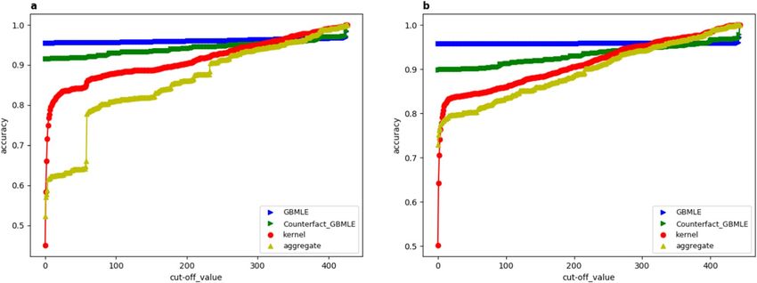
From Fig. 3a,b, the proposed GBMLE method generates the best forecast accuracy for almost all k in both the
two stages of migration, while the kernel forecast outperforms the aggregated forecast in general. This observation
verifies our theoretical prediction that the GBMLE method outperforms the kernel method by incorporating the
game structural information, while they both dominates the aggregate method because they both distinguish
the migrant-level heterogeneity while the aggregated method does not.
In addition to the overall accuracy, it is also impressive that the GBMLE forecast accuracy can reach its maxi-
mum even when k is fairly small, while the average accuracy exceeds 95% at k = 1. In the other words, there is
at most 5% chance by which the maximum-a-posteri forecaster would mistakenly pick one destination out of
400 alternative destinations. In contrast, the maximum-a-posteri forecast by the kernel method and aggregate
method would have 50% chance of making mistakes. This difference is striking and it demonstrates the power
of adding the game structural information in increasing the forecastibility.
By the green lines in Fig. 3a,b, we make a counter-fact experiment. The purpose is to test the forecastability
of the 1st-(2nd-)stage migration trajectories by the estimated 2nd-(1st-)stage migration game model. In details,
Scientific Reports | (2020) 10:12917 | https://doi.org/10.1038/s41598-020-68913-3 7
Vol.:(0123456789)www.nature.com/scientificreports/
Figure 3. Forecast accuracy for two-stage migrations In the two figures, the horizontal axis represents the
cut-off value k for the top k forecast introduced in the main text, the vertical axis represents the accuracy
rate, therefore, each curve in the two figures presents the variation trend of out-sample forecast accuracy of
a given method along with the parameter k. (a,b) Represent the stage (1) and (2) migration, respectively. The
red and yellow lines represent the forecast accuracy generated by the kernel method and aggregated method.
The blue line is the accuracy curve generated by the proposed GBMLE method. The blue line in both (a,b) are
generated by the same set of training and testing sample, which means the trainning sample used to estimate
game parameters are drawn from the same population to the testing sample used to evaluate the accuracy. In
the other words, in (a) both the training and testing sample to generate the blue line are drawn from the stage
(1) migration data, and in (b) both the trainning and testing sample are drawn from the stage ii) migration data.
In contrast, the green lines in (a,b) sketch the accuracy of GBMLE by using counter-fact trainning and testing
sample. In (a) the game parameters are estimated from the trainning sample drawn from the stage (2) migration
while the accuracy is evaluated by the stage (1) testing sample, in (b), the opposite holds, the game parameters
are estimated from the stage (1) training sample while the accuracy is evaluated by the stage (2) testing sample.
when generating the green line in Fig. 3a, the model parameters are the same as those used in generating the blue
line in Fig. 3b which are estimated from the migration data at stage (2), rather than from the “correct” stage (1).
The relation between the green line in Fig. 3b and the blue line in Fig. 3a is the same. Compare the green with
the blue line in Fig. 3a(b), we find that although the forecast accuracy by GBMLE is a bit lower after replacing
the model parameters, it is still significantly higher than the alternative methods (they are not affected by the
parameter change). Moreover, the accuracy for the maximum-a-posterior forecast by GBMLE in the parameter-
change case can still be around 91%, which has been good enough and is not much different from the case that
“correct” parameters are used. Therefore, it can be expected that the underlying mechanisms driving the observed
migration are not significantly distinct for the two stages, and migrants’ behavior is highly consistent over time.
This finding is very striking, because according to the model set-up, this finding implies a kind of “where-they-
stand-depends-on-where-they-sit” decision pattern: given that the migrant-level features are identical for two
migrants A and B while their original cities, CA and CB, are different, if A migrated to CB during the first stage,
then the decision pattern of A in choosing the second-stage destination would be analogous to the decision
pattern of B in choosing the first-stage destination while differs from A itself during the first-stage decision. In
the other words, the labor migration dynamics revealed by our data follows a Markovian decision process, i.e.
when all others equal, only the current destination matters the migration in the future, the home town does
not. This finding presents a positive evidence for the use of markovian models in describing human migration
dynamics33,50. Finally, note that the observed “where-they-stand-depends-on-where-they-sit” decision pattern
and the markovian property relies heavily on controlling the migrant-level heterogeneity. Without including
the social-economic features of migrants, the feature-dependent migration probabilities reduce to the entries
in the aggregated migration adjacency matrix which are significantly distinct for the two migration stages by
Fig. 1, therefore, the markovian properties is not detectable unless the migrant-level heterogeneity is involved.
This fact validates the usefulness of our model.
Migration inefficiencies and polarization of migrants distribution. We ask whether the observed
migration is efficient and how the degree of efficiency (measured by Eq. 4) varies in reaction to the migrant types
and migration stages. To this end, we plot the overall inefficiency
network [calculated by entry-wisely integrating
equation (4) over all migrant-level features i.e. DEX := { |X1 | x∈X DEx,ij } with | · | representing the cardinality,
X the set of all migrants having the given feature] in Fig. 4a,b for the two migration stages from which it is visual-
ized that the spatial distribution of the positive/negative signs of the inefficiency arrows and the arrow strengths
(corresponding to the sign and absolute value of entries of the inefficiency matrix (4)) are almost identical for
both of the two migration stages. The stability of the migration inefficiency is also verified by Fig. 4c–e where
we plot the aggregated two-stage migration inefficiency against different education, income and age types. It
Scientific Reports | (2020) 10:12917 | https://doi.org/10.1038/s41598-020-68913-3 8
Vol:.(1234567890)www.nature.com/scientificreports/
Figure 4. Migration efficiency across different migrant groups (a,b) plot mean of the migration inefficiency
network (4) for the stage (1) and (2) migration, respectively, where the arrow always points toward the
destination of the migration flow, the size, darkness and opacity of the arrow represents the absolute mean
value of the inefficiency measure, and the blue-colored arrow implies negative mean inefficiency measure and
the red-colored implies positive mean inefficiency measure. The inefficiency is aggregated up to the city-cluster
level and every city cluster is represented by their central city. (c–e) Present the average of the mean inefficiency
measure over all city pairs within a variety of education, income and age groups, respectively. Within each of the
subfigures, we also decompose the ineffiency measure into the positive part and negative part, and take average
for each of these two parts. (f–h) Sketch the gap of the average inefficiency measure over all city pairs between
the migration stage (1) and (2), and the left-tail pvalues of the null hypothesis that the average inefficency
measure is indfference between stage (1) and (2), where the smaller pvalue means the greater confidence to take
the alternative hypothesis that the average inefficiency is lower for stage (2) than stage (1).
is shown that for the major portion of migrants in our sample, which are the migrants with education level no
more than undergraduate, monthly income no more than 42,000 and age older than 20 and younger than 50,
the variation trend of the overall inefficiency against the increasing of education, age and income are parallel for
the two stages, while the 2nd-stage overall efficiency are systematically higher than the 1st-stage by a constant
which reflects as the aggregated inefficiency measure (Eq. 4) in Fig. 4c–e is lower in stage (2). In order to measure
the significance of the difference, we conduct the left-tail Z test and the result in Fig. 4f–h shows that at the 5%
confidential level, the inefficiency measure in stage (2) is significantly lower than that in stage (1) for the major-
ity portion of migrants. In addition, we apply ANOVA to test the significance of the parallel difference trend, it
shows that within the same range of education levels as above, we cannot reject that the 2nd-stage inefficiency
Scientific Reports | (2020) 10:12917 | https://doi.org/10.1038/s41598-020-68913-3 9
Vol.:(0123456789)www.nature.com/scientificreports/
curve in Fig. 4c differs from the 1st-stage inefficiency curve by a constant even at the 20% confidential level, the
same holds for age and income as well which provide positive evidence for the parallel trend.
The increasing migration efficiency is quite intuitive and consistent with the job searching theory51 since the
first-stage migration helps accumulate more information of the potential destinations that facilitates migrants to
make rational decision. The relative invariance of migration efficiency against the variation of multiple migrant-
level features is quite surprising. One possible explanation for this observation is the invariance of the migration
game which is supported by Fig. 3, because the identical game set-up implies the same functional form of g which
defines the ideal population ratio of each destination and also consists of a key component of the inefficiency
measure (4). Hence, the invariance of g provides a stablizer for the two-stage migration inefficiency.
Finally, it is observed from Fig. 4c,d a decreasing trend of migration inefficiency along with the increasing
of education and income at least for the majority population (education level less than the master’s degree and
monthly salary less than 42,000). This observation implies that high-educated and well-paid migrants tend to
make more rational decision in selecting destination which agrees with the l iterature52 that high education can
increase the decision rationality and the fact that the high income are often the consequence of high education.
Classification of destinations and education‑chasing behind migration dynamics. From Fig. 4,
it is clear that in both of the two migration stages, the overall efficiency is poor (reflected as the inefficiency meas-
ure is significantly positive for both stages). Then it is natural to ask what causes the inefficient migration. To
answer that question, we notice that there are two sources leading to the positive inefficiency measure by defini-
tion equation (4): (1) a migrant is more likely to migrate to a destination than the average even if the given desti-
nation is already over-sized in his/her view; (2) a migrant is less likely to migrate to a destination than the aver-
age while the destination can better off if more migrants can come in. Similarly, the negativity of the inefficiency
measure also arises from two sources that are exactly opposite to the two above. Given that, all destination cities
can be partitioned into four classes: (I) the np cities that consist of the unsaturated cities (with i DEx,ij 2 < 0)
with positive aggregated flow-ins ( i DEx,ij 1 > 0); (II) the nn cities that consist of the unsaturated cities (with
i DEx,ij < 0) with negative aggregated flow-ins ( i DEx,ij < 0); (III) the pn cities that consist of the oversized
2 1
cities (with i DEx,ij > 0) with negative aggregated flow-ins ( i DEx,ij
2 1 < 0); and (IV) the pp cities that consist
of the oversized cities (with i DEx,ij 2 > 0) with positive aggregated flow-ins (
i DEx,ij > 0).
1
We ask what is the major feature of the four classes of city, how do they differ from each other and how is
the difference related to the inefficient migration pattern? To this end, we consider the seven city-level features:
population, GDP, foreign direct investment (FDI), total road length, city building area, the total number of
teachers in all primary and middle schools and the total number of beds in all hospitals. The seven features are
devoted to capture the social-economic development level of a city, among which the number of teachers and
beds are proxies to the education and healthcare resources, which are two most important public goods and very
influential to migration decision35–37,53. The city-level feature data is collected from Chinese Statistical Yearbook
(2015) which are only available for the 178 cities in the 21 city clusters, so the aggregation is also taken on that
basis. Fig. 5a–c present the mean of the seven features within each city class where the city classification and
mean features are calculated for the overall inefficiency measure (integrating DEx,ij 1 , DE 1 with respect to all i
x,ij
and x) and for both migration stages.
Since the inefficiency measure (Eq. 4) is defined on the level of migration flow between city pair, the four
classes of cities can even be extended to the set of all migration flows, which becomes four classes of ordered city
pairs. For each of the city-pair classes, we compute the OD ratio of the seven features which are ratios formed by
dividing the value of the origin city at a certain feature dimension by that of the destination city. The OD ratios
convey more information than the absolute value of city-level features because they encode the comparison
between the origin and the destination cities. The mean OD ratio for the four city-pair classes and its variation
along with education, age and income are plotted in Fig. 5d–f (in Supplementary Fig. S10, we plot the radial
graph for the mean features and OD ratios for the per capita value of the six features other than population,
which is the quotient by letting the feature value divide the population, which shows a qualitatively identical
pattern to the Fig. 5).
The geometric shape of the feature area within each of the radial plots in Fig. 5 are quite identical for both
migration stage (1) and (2), this observation supports, once again, the invariance of the migration game. For the
mean features and OD ratios of the city classes, some remarkable properties can be concluded. First, compared
to the unsaturated cities (the nn and np class in Fig. 5a,c), the oversized cities (the pn class in Fig. 5b) are signifi-
cantly greater in both migration stages and in all of the seven city-level features. This finding is not trivial because
except for the 22 city-cluster dummy variables, no city-level social-economic feature is included when fitting
the migration game. In the other words, the classification by the migration data can have a perfect match to the
real social-economic gap between the “large” and “small” cities even though the social-economic data of cities
are missing from the classification process. This result establishes a natural link between the migration behavior
and the city “size” which suggests a novel way to describe the “largeness” or “smallness” of a city.
Second, the np class differs from the nn class mainly in the stock of education resources measured by the num-
ber of teachers in primary and middle school and the np class of cities tend to own better education resources.
This fact is robust for both migration stages, and can even be reinforced through comparing Fig. 5d,f where the
relative advantage on the teacher’s number is much more significant for those np city pairs. The right-tail Z test
is conducted to measure the significance of the finding for a variety of migrant types, the result shows that the
teacher’s number is always significantly higher in the np class at the 0.05 confidential level for almost all situations
(see Suplementary Fig. S3). In contrast, the other features, such as the healthcare resources measured by the bed
number, do not differ much between the nn and np classes (see Supplementary Figs. S4–S9). The extraordinary
Scientific Reports | (2020) 10:12917 | https://doi.org/10.1038/s41598-020-68913-3 10
Vol:.(1234567890)www.nature.com/scientificreports/
Figure 5. Features of four city classes (a–c) present the radial plot for the means of the seven city-level features
for the nn, pn and np class of cities respectively for both stages of migration; (d–f) present the radial plot for the
mean OD ratios of the seven city-level features for the nn, pn and np class of city pairs respectively for the two
stages of migration. Because the pp class contains no city nor city pair for both stage (1) and (2) migration, the
relevant radial plots are missing. During the classification, to avoid the data noise, we trimed those very small
valued DEx,ij
1 and DE 2 in the sense of setting DE 1 (DE 2 ) as 0 when their absolute value is less than 0.001,
x,ij x,ij x,ij
then the resulting city pair ij is discarded as noisy point and will not be rendered into any of the four classes.
role played by education resources in attracting migrants results deeply from the fact that the education resources
are immobile which makes migration the only way to chase better education54. Although the healthcare resources
have the similarly immobile nature, it cannot impact the migration as much as the education resources because
living temporally is fully feasible to take use of the healthcare services in a different city, there is no need to induce
observable migration flow. In contrast, schools will not provide service unless migration really happens. In that
sense, the education resources are more immobile than the healthcare resources, therefore offering better edu-
cation services could form a long-lasting comparative advantage of a city in attracting migrants, this advantage
will not leak out and be “freely” used by non-migrants.
Finally, the comparative disadvantage of nn class in education resources also provides an explanation to the
overall inefficient migration pattern. In fact, around 4/5 of all ordered city pairs are contained in the nn class,
which dominates all the other three classes and constitutes the main portion of the inefficient migration arrows in
Fig. 4a,b As the nn class of city (pairs) are caused by the relative shortage of education resources in the destination
cities, it is reasonable to claim that the imbalanced spatial distribution of education resources is a major driving
force of the overall inefficient migration. This finding is consistent with the existing studies on the relationship
between Chinese labor migration and the education s ystem40, and provides positive evidence for the argument
that the distortion on education induces the distortion of population migration.
Discussion
To summarize, we study a large migration game model that can be fitted with real data through a constrained
maximum likelihood procedure. From the game model, the conditional migration probability among the set of
destinations can be naturally identified with a mixed-strategy Nash equilibrium of the game. The migrant-level
heterogeneity is easily embedded into the game via the feature space of migrants, as a consequence, the resulting
equilibria migration behavior is represented as a family of type-specific migration networks. Through applying
the model to a two-stage Chinese labor-force migration dataset, we find that although the network structures
are significantly distinct for two migration stages, the underlying migration game is essentially unchanged.
Given the stationary game set-up, even if a migrant can select different destinations at different stages, the
difference can only be induced by the different starting cities, which implies a “where-they-stand-depends-on-
where-they-sit” decision pattern. In the macro view, this decision pattern suggests the shuffling of migrants’
distribution be the main source of the network structural change for the 2nd-stage migration in relative to the
1st-stage one. The staionarity of the game set-up also helps stablize the migration inefficiency measure whose
distributions along with the spatial coordinate and the major migrant features turn out invariant qualitatively
for the two migration stages. In addition, we test the heterogeneity of migration network against a variety of
education, age and income types. The result shows that the migrant types can significantly alter the structure of
migration networks. This result is quite robust, indicating the necessity of incorporating migrant-level feature
Scientific Reports | (2020) 10:12917 | https://doi.org/10.1038/s41598-020-68913-3 11
Vol.:(0123456789)You can also read