Unveiling the rarest morphologies of the LOFAR Two-metre Sky Survey radio source population with self-organised maps
←
→
Page content transcription
If your browser does not render page correctly, please read the page content below
A&A 645, A89 (2021)
https://doi.org/10.1051/0004-6361/202038500                                                                            Astronomy
c ESO 2021                                                                                                              &
                                                                                                                       Astrophysics

   Unveiling the rarest morphologies of the LOFAR Two-metre Sky
     Survey radio source population with self-organised maps
      Rafaël I. J. Mostert1,2 , Kenneth J. Duncan1,3 , Huub J. A. Röttgering1 , Kai L. Polsterer4 , Philip N. Best3 ,
 Marisa Brienza5,6 , Marcus Brüggen7 , Martin J. Hardcastle8 , Nika Jurlin2,9 , Beatriz Mingo10 , Raffaella Morganti2,9 ,
                                 Tim Shimwell2,1 , Dan Smith8 , and Wendy L. Williams1

       1
           Leiden Observatory, Leiden University, PO Box 9513, 2300 RA Leiden, The Netherlands
           e-mail: mostert@strw.leidenuniv.nl
       2
           ASTRON, the Netherlands Institute for Radio Astronomy, Postbus 2, 7990 AA Dwingeloo, The Netherlands
       3
           SUPA, Institute for Astronomy, Royal Observatory, Blackford Hill, Edinburgh EH9 3HJ, UK
       4
           HITS gGmbH (Heidelberg Institute for Theoretical Studies), AstroinformaticsSchloss-Wolfsbrunnenweg 35, 69118 Heidelberg,
           Germany
       5
           Dipartimento di Fisica e Astronomia, Università di Bologna, via P. Gobetti 93/2, 40129 Bologna, Italy
       6
           INAF – Istituto di Radioastronomia, Via P. Gobetti 101, 40129 Bologna, Italy
       7
           University of Hamburg, Gojenbergsweg 112, 21029 Hamburg, Germany
       8
           Centre for Astrophysics Research, University of Hertfordshire, College Lane, Hatfield AL10 9AB, UK
       9
           Kapteyn Astronomical Institute, University of Groningen, PO Box 800, 9700 AV Groningen, The Netherlands
      10
           School of Physical Sciences, The Open University, Walton Hall, Milton Keynes MK7 6AA, UK

     Received 26 May 2020 / Accepted 29 October 2020

                                                                   ABSTRACT

     Context. The Low Frequency Array (LOFAR) Two-metre Sky Survey (LoTSS) is a low-frequency radio continuum survey of the
     Northern sky at an unparalleled resolution and sensitivity.
     Aims. In order to fully exploit this huge dataset and those produced by the Square Kilometre Array in the next decade, automated
     methods in machine learning and data-mining will be increasingly essential both for morphological classifications and for identifying
     optical counterparts to the radio sources.
     Methods. Using self-organising maps (SOMs), a form of unsupervised machine learning, we created a dimensionality reduction of
     the radio morphologies for the ∼25k extended radio continuum sources in the LoTSS first data release, which is only ∼2 percent of
     the final LoTSS survey. We made use of PINK, a code which extends the SOM algorithm with rotation and flipping invariance,
     increasing its suitability and effectiveness for training on astronomical sources.
     Results. After training, the SOMs can be used for a wide range of science exploitation and we present an illustration of their potential
     by finding an arbitrary number of morphologically rare sources in our training data (424 square degrees) and subsequently in an
     area of the sky (∼5300 square degrees) outside the training data. Objects found in this way span a wide range of morphological and
     physical categories: extended jets of radio active galactic nuclei, diffuse cluster haloes and relics, and nearby spiral galaxies. Finally,
     to enable accessible, interactive, and intuitive data exploration, we showcase the LOFAR-PyBDSF Visualisation Tool, which allows
     users to explore the LoTSS dataset through the trained SOMs.
     Key words. galaxies: active – galaxies: peculiar – radio continuum: galaxies – techniques: image processing – methods: statistical –
     methods: data analysis

1. Introduction                                                             this separation and the Fanaroff-Riley class II (FRII) sources
                                                                            being systematically above it.
The morphology of a radio source is an important tool for                       A new generation of radio surveys, such as the Low Fre-
studying the nature of the source emitting the radio waves and              quency Array (LOFAR; van Haarlem et al. 2013) Two-metre
the environment or medium around the radio-emitting source                  Sky Survey (LoTSS; Shimwell et al. 2017), the Evolution-
(e.g. Miley 1980; Kempner et al. 2004). In radio astronomy,                 ary Map of the Universe (EMU; Norris et al. 2011), and the
the most time-resistant morphological classification scheme for             MeerKAT international GHz tiered extragalactic exploration
radio galaxies is the one presented by Fanaroff & Riley (1974),             (MIGHTEE; Jarvis et al. 2016) are producing ever larger sam-
which classifies radio galaxies based on their extended radio               ples of highly resolved radio sources. Furthermore, LoTSS com-
jets. The binary classification scheme is based on the location             bines high angular resolution with a high sensitivity to diffuse
of the brightest hot-spots within the lobes of an extended source.          radio emission, which has never been achieved before over large
Fanaroff & Riley (1974) used their scheme to classify a num-                area surveys, and thus it probes a different range of morpholo-
ber of sources from the revised third Cambridge catalogue of                gies (e.g. Hardcastle et al. 2019; Mandal et al. 2020. The extent
radio sources (3CR; Mackay 1971) and found a distinct separa-               to which these new radio surveys may redefine our understand-
tion in the luminosities of these sources at 2×1025 W Hz−1 sr−1 at          ing of radio morphology is illustrated by the recent results of
178 MHz, the Fanaroff-Riley class I (FRI) sources being below               Mingo et al. (2019), who find that the dichotomy between FRI

                                                        Article published by EDP Sciences                                          A89, page 1 of 22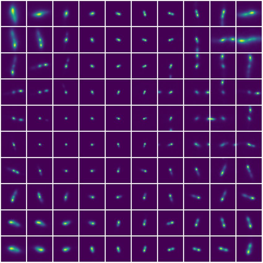
A&A 645, A89 (2021)

and FRII luminosities does not seem to hold (supporting Best           an approach that minimises our assumptions and any biases
2009) and that the radio active galactic nuclei (AGN) population       inherent within them.
might be more heterogeneous than previously assumed.                        In this paper we use a rotation and flipping invariant imple-
    Radio morphological information is also used when perform-         mentation of the self-organised maps (SOM; Kohonen 1989,
ing optical or infrared cross-identifications, providing us with       2001) dimensionality reduction algorithm (Polsterer et al. 2015)
valuable information on the nature of the radio sources. For unre-     to explore the morphologies of radio sources in the LOFAR Two-
solved radio sources, if present, a host galaxy should be located      metre Sky Survey First Data Release (Shimwell et al. 2017).
at the same location as the radio emission. For resolved radio         The dimensionality reduction will be a model that represents
AGN, we expect a host galaxy to be at the origin of its jets. This     the most frequently occurring shapes in our data, regardless of
origin is not necessarily close to the flux-weighted centre of the     whether they conform to any pre-existing morphological clas-
radio emission. In these cases, we need to use morphological           sification scheme. In addition to providing a data-driven model
information (the orientation of the jets projected onto the sky        of the representative radio morphologies within LoTSS, an SOM
plane) to find the potential host galaxy.                              can be used to select the radio objects that most diverge from this
    A classical classification of radio morphology consists of         model – these will be morphologically rare or outlier sources that
automated source detection (using a simple signal-to-noise cri-        can automatically be identified within potentially unexplored
terion), followed by a manual label process. With the LOFAR            parameter space. This method does not limit our search to many
surveys and the future surveys of the Square Kilometer Array           forms of AGN (bent, assymetric, remnant and restarted), it also
(SKA; Schilizzi 2004) and its pathfinders, it is essential to          leads us to nearby spiral galaxies and cluster emission many of
explore methods in machine learning and data-mining to deal, in        which may be previously undiscovered in radio observations.
a more automated and therefore inherently statistical way, with        We do not tackle the FRI or FRII classification of LoTSS radio
the large sample coming our way.                                       sources in this paper as this requires additional completeness
    Conveniently, in the past few years, in the field of computer      simulations.
science, significant improvements have been made in the fields              This paper is set out as follows: Sect. 2 presents the LOFAR
of data mining and machine learning in general and computer            radio continuum dataset used in this work. Section 3 introduces
vision specifically. These improvements are generally recog-           the rotation and flipping invariant SOM technique and outlines
nised to be enabled by the availability of larger datasets, increas-   its application to the LoTSS sample of radio continuum sources.
ingly powerful graphics processing unit (GPU) accelerated com-         Section 4 presents the resulting trained SOMs, including the
pute power and the development and refinement of machine               range and distribution of morphological representative images
learning algorithms (e.g. Halevy et al. 2009; Goodfellow et al.        within the LoTSS extended radio source population. We illus-
2016; Sun et al. 2017).                                                trate how the trained map can be used to automatically identify
    We can roughly divide machine learning approaches into             morphologically unique sources in new datasets. In Sect. 5 we
two categories: supervised and unsupervised learning (e.g.             discuss our research and its place within the wider picture of
Goodfellow et al. 2016). Supervised approaches are fundamen-           large survey science. Finally, Sect. 6 presents the summary and
tally limited by the requirement for a labelled training sample,       conclusions of the paper.
which can be limited in size, or by the fact that such a sample
is only available for certain surveys. Human-created labels or
human-annotated data are valuable but costly as the annotation         2. Data
process scales linearly with the number of samples in a dataset.
Unsupervised learning does not require labels for its training         The primary data used for training and optimising the SOMs
dataset and can be used for density estimations or to cluster data     in our study is taken from the first data release of the LOFAR
in groups according to patterns in the data (e.g. Goodfellow et al.    Two-metre Sky Survey (LoTSS-DR1; Shimwell et al. 2019) and
2016). The lack of labels means these techniques are not biased        consists of 58 pointings that make up a mosaic that covers 424
by preconceived human-created categories; however, they do not         square degrees in the HETDEX region of the sky (right ascen-
necessarily relate to intrinsic physical source properties.            sion 10h45m00s–15h30m00s and declination 45◦ –57◦ ). The sur-
    Unsupervised learning approaches have been applied to              vey, observed at 120–168 MHz with a median rms sensitivity of
astronomical datasets before. Baron & Poznanski (2016) took an         S 144 MHz = 71 µJy beam−1 and a resolution of 600 , will eventually
unsupervised approach to study galaxy evolution by using ran-          cover the entire Northern sky.
dom forests to find spectroscopic outliers in the Sloan Digital            The data are accompanied by a corresponding catalogue
Sky Survey (SDSS). Segal et al. (2018) used “apparent complex-         containing 352 694 source-entries, generated by the Python
ity” as a metric to describe radio morphology. In this approach,       Blob Detection and Source Finder (PyBDSF)1 application
images of radio sources are compressed using the gzip com-             (Mohan & Rafferty 2015); see Shimwell et al. (2019) for the
pression algorithm after which the size of the resulting file is       parameters used. PyBDSF builds a catalogue from emission
a course-grained measure for the morphological complexity of           islands with peak intensity values that exceed the surrounding
the source. The one-dimensional nature of the result makes it a        noise in the image by, in this case, five standard deviations. One
potentially useful addition to a catalogue where it can serve as       or more Gaussians are fit to these islands. If these Gaussians
input to supervised learning methods. On its own, the metric is        overlap2 , they will enter the catalogue as a single entry. The
not so valuable, as the degeneracies are numerous and no infor-        RA and Dec of the entry is set to the centroid of its Gaussians,
mation about the shape, size or number of components of the            which is determined using moment analysis. 93% of the cata-
source is retained.                                                    logue entries correspond to unresolved sources. As these contain
    Our ultimate aim is to robustly classify the radio sources in      no morphological information beyond an upper limit on their
new generations of wide and deep radio surveys according to
their morphology. Given the new parameter space being probed           1
                                                                         https://github.com/lofar-astron/PyBDSF
by these surveys and the potential new morphological regime            2
                                                                         Grouping of Gaussians into sources: http://www.astron.nl/
they reveal (Mingo et al. 2019), unsupervised clustering offers        citt/pybdsf/algorithms.html#grouping

A89, page 2 of 22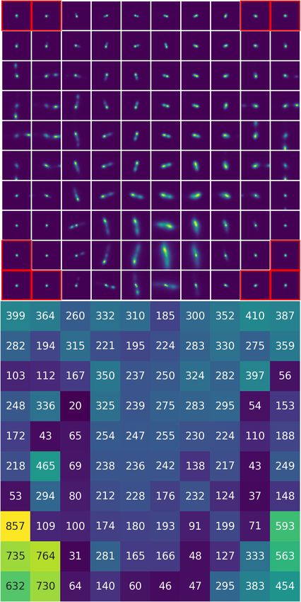
R. I. J. Mostert et al.: Unveiling radio morphology using self-organising maps

angular size, we only train on the 24 601 objects composed of             while the hyper-parameters are set (and may be updated) by the
multiple Gaussians3 .                                                     user. The pixel-values of the representative images are model
    In Sect. 4.4, we make use of additional LoTSS data consisting         parameters, the dimensions of the SOM lattice and the dimen-
of 841 pointings that make up a mosaic that covers 5720 square            sions of the cutouts are hyper-parameters.
degrees, fully overlapping with the 424 square degrees of the                 For a full outline of the SOM algorithm and its basic imple-
HETDEX region of the sky. This dataset, constitutes the second            mentation, we refer the reader to Kohonen (2001). In the next
LoTSS data release (LoTSS-DR2; Tasse et al. 2020) and contains            section we describe the rotation and flipping-invariant SOM
4 395 448 PyBDSF-generated source-entries. We use the part of             algorithm employed in this work and subsequently its hyper-
this larger dataset that is outside our initial dataset to show that an   parameters.
SOM trained with sources on a small patch of the sky can be used
to cluster and find outliers in sources from a different part of the
                                                                          3.1. Rotation invariant SOM
sky without retraining.
                                                                          The classification of radio source morphologies should not
                                                                          depend on the orientation of the source on the sky. Hence, the
3. Method: Rotation invariant self-organised maps                         classification should be invariant to rotation and flipping. Even
A self-organising map (SOM; Kohonen 1989, 2001), also known               so, most algorithms, supervised or unsupervised, are not fully
as a Kohonen self-organising map, Kohonen map or Kohonen                  rotation and flipping invariant. For supervised convolutional neu-
network, is an unsupervised artificial neural network used to             ral networks this problem is often handled by simplified approx-
reduce high-dimensional data to a low-dimensional (usually two            imation by inserting (many) rotated copies of each source in
or three) representation (known as the “map” or the “lattice”).           the training dataset (e.g. Dieleman et al. 2015; Aniyan & Thorat
An SOM belongs to the family of dimensionality reduction tech-            2017; Alhassan et al. 2018; Dai & Tong 2018; Lukic et al. 2018,
                                                                          2019).
niques and is an especially useful starting point for visualisa-
tion and clustering and hence data-exploration. An SOM aims                   Polsterer et al. (2015) proposed a rotation and flipping
to capture the properties of the elements of a dataset by creat-          invariant SOM algorithm:
                                                                              1. Initialise the pixel-values of the images in the adopted lat-
ing a small number of representative elements on a fixed lattice.
                                                                          tice to some arbitrary value. In our case we initialise with zeros.
One key property of SOMs that makes them particularly use-
ful for morphological studies is that they are coherent; similar              2. For each image in the training dataset:
representative images should be close to each other on the lattice            (a) Create rotated and flipped copies.
while dissimilar representative images should be further apart on             (b) For each representative image Rep, calculate the
the lattice.                                                              Euclidean norm to each of the copied images Imcopy in the SOM,
     Our dataset consists of cutouts from Stokes-I LOFAR                  where the Euclidean norm is defined as:
images, with each cutout centred on a radio source that has                                     sX
been detected in the associated PyBDSF source catalogue (see              kImcopy − Repk2 =           (Imcopyi − Repi )2 ,                 (1)
Sect. 3.2 for details). Thus our SOM should capture the overall                                    i
properties of the images in our dataset by creating a small num-
ber of representative images on a fixed lattice. Formally, an SOM
consists of a lattice of “neurons” and each neuron has weights            and the summation is over all the pixels i of the images.
(pixels of the representative image). By iteratively training these            (c) For each representative image, find the image copy
weights (the pixels of the representative images will be itera-           Imcopy,best to which it has the smallest Euclidean norm. If mul-
tively adjusted), the aim is to maximise the similarity between           tiple image copies produce the same norm, randomly select one
the neurons (images) and the training dataset.                            of those image copies.
     The metric we use for determining the similarity between a                (d) From the set of image copies to each representative image
representative image and an image from the training dataset is            found in 2c, find the single combination of representative image
the Euclidean norm, meaning that we subtract the representa-              and copied image Imcopy,best that have the smallest Euclidean
tive image from the image in the training dataset and take the            norm to each other. We refer to this representative image as
square root of the squared sums of the pixel values in the resid-         Repbest . If multiple combinations produce the same norm, ran-
ual image. By minimising the value of the norm of each image in           domly select one of those combinations. Repbest,loc denotes the
the training dataset to its corresponding most similar representa-        (x, y) location of Repbest on the SOM lattice.
tive image, we ensure that the representative images of the SOM                (e) Update the pixels of each representative image Rep such
are a good representation of the images in the training set.              that they are more like their respective Imcopy,best :
     For determining the coherence we count the number of
images in our training dataset for which the second best match-           Repnew = Rep + α · θ kRepbest − Reploc k2

ing representative image is not located directly next to the best                  · (Imcopy,best − Rep),                                 (2)
matching representative image on the lattice. By minimising this
number we ensure that the SOM is coherent.
     In machine learning, the distinction is made between model           where Repnew is the updated representative image, α is a scalar
                                                                          known as the learning constraint and θ kRepbest − Reploc k2 is a

parameters and model hyper-parameters. Model parameters are
initialised by the user and updated by the training algorithm,            function known as the neighbourhood-function. We note that α
                                                                          regulates to what degree all representative images should adapt
3
  That is, entries with PyBDSF S_Code = “M” or “C”. See http://           to Imcopy,best ; θ is a function of the Euclidean norm between the
astron.nl/citt/pybdsf/write_catalog.html#write-catalog                    location of the considered representative image on the lattice
and http://astron.nl/citt/pybdsf/algorithms.html#gauss                    Reploc and Repbest,loc . It causes representative images that are
ian-fitting                                                               farther apart from Repbest,loc on the lattice to adapt less to their
                                                                                                                            A89, page 3 of 22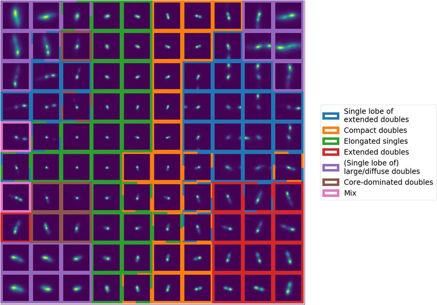
A&A 645, A89 (2021)
respective Imcopy,best . We chose the boundaries of the SOM to be representing slightly bent extended doubles. For this paper we
periodic4 . adopt a 10 × 10 lattice. SOMs can be trained on a lattice with
3. Repeat step 2 (except for 2a) a fixed number of times (or more than two dimensions, but in this study we make use of only
“epochs”) or until a user-defined stopping condition is met. two-dimensional SOMs, as higher dimensional SOMs are harder
4. Now that the SOM is trained, optionally repeat step 2b to visualise on a 2D surface.
and 2c once. Then for each image, return the smallest Euclidean For the neighbourhood-function PINK adopts a commonly
norm of each representative image to their Imcopy,best . used 2D-symmetric Gaussian of the form
Polsterer et al. (2015) developed PINK5 , a GPU-optimised
code for step 1, 2 and 4 of this algorithm. In this study we 1
θ(σ, Repbest , Reploc ) = √
build on the core PINK algorithm to appropriately preprocess σ 2π
LOFAR data for PINK version 0.23 and enable automated and !2
1 kRepbest − Reploc k2
flexible implementation of step 3 such that θ and α are scalar · exp − , (4)
functions that also depend on the number of completed epochs. 2 σ
For SOMs, tuning hyper-parameters comes down to a trade-
off between compute-time, how similar the images in our dataset where σ is known as the neighbourhood radius. Generally a
are to the representative images in the (trained) SOM and the larger neighbourhood radius will result in a lower TE and higher
coherency across the SOM. Good coherence implies that the AQE. We can intuitively understand this, as a larger neighbour-
similarity between the representative images decreases gradually hood radius will cause each training image to leave its imprint
as a function of distance on the lattice between them. on a larger part of the SOM lattice and as a result, represen-
To quantify the coherency of the SOM and how similar the tative images will be more similar across the lattice: creating
images of our dataset are to the representative images in the better coherence but with the representative image set encom-
(trained) SOM, we used two metrics. The Average Quantisation passing less well the variety of images in the dataset. As stated
Error (AQE), as described by Kohonen (2001), is defined as the by Kohonen (2001), by decreasing the neighbourhood radius
average summed Euclidean norm from each image in our dataset with each training epoch, updates to the lattice will at first be
to its corresponding best matching representative image: global (ensuring coherence) and then become ever more local
|D| , (ensuring a good representation of the individual images in our
X dataset). Therefore, we adopt and implement a decrease in the
AQE = kImcopy,best − Repbest k2 |D|,
(3) neighbourhood radius such that σ(t) = σ0 × σtd with t the epoch
number, σ0 the starting radius and σd the radius decrease rate.
where the summation iterates over all images in our dataset D For the value of σ0 , we adopted the rule of thumb from Kohonen
and |D| is the number of images in our dataset. A lower AQE (2001): we start with a neighbourhood radius half the size of the
equals a better representation of the data. The Topological Error largest dimension of the SOM lattice.
(TE) as described by Villmann et al. (1994), is a measure for the The size of the learning rate α determines the size of the
coherence of the SOM. It is defined as the percentage of images step we take in the model-landscape. Small steps will generally
for which the second best matching representative image is not slowly take us in the right direction but can get us stuck in a local
a direct neighbour of the best matching representative image, optimum, while big steps give faster results but might overshoot
where direct neighbour is defined as all eight neighbours for rep- the (local) optimum. The best results within a given compute-
resentative images on a rectangular lattice. A lower TE equals time is achieved by starting out with a large value for the learn-
better coherency. We note that AQE and TE are relative measures ing rate and gradually decreasing its size with every epoch. We
and can only be used to monitor progress of an SOM during adopt and implement √ a decrease in the learning rate such that
training (for example after every completed epoch) or to make a α(t) = α0 ×αtd ×σ(t) 2π with t the epoch number, α0 the starting
comparison between different SOMs that have been trained with learning rate and αd the learning rate decrease. We also use the
the same dataset and the same image and lattice dimensions. learning rate to undo the normalisation of the neighbourhood-
A dimensionality reduction technique can produce a closer function: we keep its peak constant at the value of 1. If we were
approximation of a dataset when given more model parameters to keep the 2D-Gaussian normalised, for small neighbourhood
to model this dataset. For an SOM, having more representative radii, the impact of a single training image on the representa-
images is equivalent to more model parameters. Therefore, an tive images of the SOM would be too great. For each subsequent
SOM with more representative images leads to a better repre- image, the best matching representative image would be updated
sentation of the images in the training dataset (lower AQE and to be very much like this image, thereby erasing the similarity to
TE). The size of the SOM lattice is arbitrary and we can change it previous images.
in accordance with the purpose of the dimensionality reduction. To determine reasonable values for the SOM lattice dimen-
Using hundreds of representative images for the visual inspec- sions, σd , α0 and αd , we tested the SOM algorithm and its
tion of the most common morphologies in the data is impracti- hyperparameters on the well known MNIST handwritten dig-
cal, and a small trained lattice (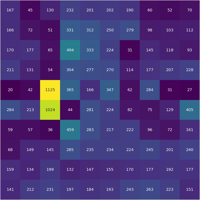
R. I. J. Mostert et al.: Unveiling radio morphology using self-organising maps

Table 1. Parameters used for the first SOM training run.

                   SOM lattice dimensions (w × h × d)                                     10 × 10 × 1
                   Number of channels or layers                                                 1
                   Representative image dimensions                     67 × 67 pixels2 , equivalent to 100 × 100 arcsec2
                   Neighbourhood radius start σ0 | decrease σd                               5 | 0.9
                   Learning rate start α0 | decrease αd                                      1 | 0.7
                   Periodic boundary conditions                                               True
                   Stopping condition                                        AQE improvement per epoch < 1%
                   Resulting number of training epochs                                         23
                   Initialisation                                                            Zeros

    At the start of the training process, we initialise the pixel-                                1.00
values of our representative images with zeros. Different initial-
isation, for example using random numbers, changes the initial                                    0.95
place on which the images leave their inprint on the SOM. As we

                                                                          Percentage of sources
train for more than 20 epochs, the initialisation – given it is of                                0.90
similar magnitude to the training images – only leads to changes
in the final location of the groups we find. It does not expose new                                                          all sources
                                                                                                  0.85                       multiple Gaussian component sources
morphological groups.
                                                                                                  0.80
3.2. Preprocessing: Creating a training dataset from LoTSS
     images                                                                                       0.75

Our training set only contains images – no labels, or catalogue                                   0.70
information, just pixel-information. We created images for our                                           0   50        100            150           200       250
                                                                                                              FWHM of major axis of source [arcsec]
training dataset by making a square cutout from the LOFAR
intensity maps for each catalogue entry. Each cut-out has a fixed        Fig. 1. Cumulative distribution function (CDF) of the full-width half
angular (or on-sky) size, centred on the source right ascension          maximum (FWHM) of the 325 694 radio-sources in the catalogue and
and declination. We proceeded by applying a circular mask,               the subset of 24 601 sources that are composed of multiple Gaussians
removed all flux below 1.5 times the local noise and rescaled            by PyBDSF. The reported FWHMs of the sources are on the low side
the remaining flux to the continuous Adelman-McCarthy (2009)             as PyBDSF breaks up large apparent objects into multiple catalogue
                                                                         entries with smaller sized objects.
range. Below we elaborate on these steps.
    Given the varying intrinsic physical sizes and redshifts of
the radio source population, the choice for the on-sky size is
thus a cause of degeneracy in our trained SOM. Sources with
similar morphology but different apparent size will best match           small enough to minimise the amount of nearby unrelated radio
different neurons on the SOM. Using different on-sky sizes for           emission. Ideally, we would remove the emission from neigh-
each source and then rescaling the dimensions of each image              bouring sources that spuriously entered our image. This is not
such that the extent of the radio emission for all resolved sources      practical due to the difficulty of correctly associating emission
spans a fixed number of pixels would avoid this issue. However,          with a single radio source. Our source might be part of a larger
this is not a trivial task for several key reasons. Firstly, a radio     structure which we risk incorrectly removing (i.e. our catalogue
source can consist of two lobes of emission that are spatially sep-      entry might be centred on a single lobe of a double-lobed radio
arated, such that automatic source extraction software is not able       source in which case we would remove the second lobe). Limi-
to recognise that the two islands of emission belong to a single         tations to the fixed image size are discussed in Sect. 5.1.
radio source. The source size reported by source extraction soft-            We informed our decision process by gathering information
ware may thus refer to a small emission structure that is part of        on the nearest-neighbour distances of all 325 694 radio-sources
a larger structure. Secondly, the precise size or extent of a radio      in the catalogue and the different sizes of all 24 601 multiple-
source has no fixed definition and will also depend on the mor-          component objects that we used for training. Figure 1 indicates that
phology itself. We refer the reader to Sect. 5.1 for more on this        a cutout size between roughly 50 and 150 arcsec is able to encom-
topic.                                                                   pass most extended sources as reported by the catalogue. Figure 2
    In the remainder of this paper, we proceed to use fixed on-sky       shows that avoiding any contamination from unrelated sources
size images to train our SOM. Using fixed on-sky size images,            is impossible; we should at least stay well below 200 arcsec
the SOM will need more neurons to represent the images in                to avoid contamination in virtually all cutouts. We adopt a fixed on-
the training dataset compared to the ideal case where the extent         sky size of 100 × 100 arcsec2 , which translates into 67 × 67 pixel2
of the emission is normalised. Nevertheless, after training, the         images as the pixel scale of our FITS-files is 1.5 × 1.5 arcsec2 .
SOM will still be a good representation of the images in the                 In the rotation procedure of the training algorithm (step 2a)
training dataset. Compared to regular sources, sources with out-         we create image copies that are flipped and rotated by incre-
lying morphologies will still have a larger Euclidean norm with          ments of 1 degree using bilinear interpolation. Including flip-
respect to the weights of their best matching neurons.                   ping we end up with 720 rotated and or flipped image copies for
    To capture most of the source morphology, the fixed on-sky           each image in our training dataset. To ensure that these images
size should be chosen big enough that most sources fit inside and        do not have empty corners, initial images of 95 × 95 pixels2

                                                                                                                                                 A89, page 5 of 22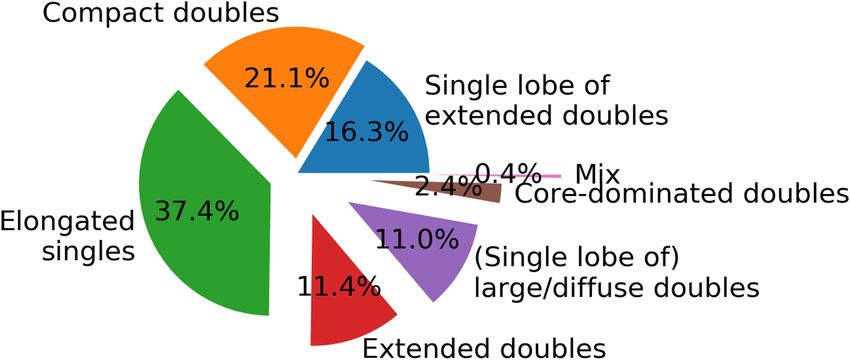
A&A 645, A89 (2021)

                        1.0                                                                              this study is to find rare morphologies across the full dynamic
                                                                                                         range of LoTSS, we therefore normalise the intensity of all
                                                                                                         sources by linearly scaling the intensity values of each image
                        0.8                                                                              in our training dataset to between 0 and 1 (after sigma-clipping).
Percentage of sources

                                                                                                         During training, because of the rotation and subsequent crop-
                        0.6                                                                              ping, only the pixels within the circle with a diameter equal to
                                                            all sources                                  the width of our image are used to compare the image to the neu-
                                                            multiple Gaussian component sources          ron weights. Therefore, we only consider these pixels during the
                        0.4                                                                              intensity rescaling and mask all pixels outside of this circle.
                                                                                                             In future research simultaneous training on multiple layers
                        0.2                                                                              will be considered: multiple instances of the same image with
                                                                                                         different scaling or clipping applied to highlight different fea-
                                                                                                         tures of each source. See Sect. 5.3 for a description of a multi-
                        0.0                                                                              layer SOM.
                                  0   100     200      300       400      500      600     700
                                        Angular distance to nearest neighbour [arcsec]
Fig. 2. CDF of the angular distance to the nearest neighbour for                                         4. Results
all 325 694 sources and for the subset of 24 601 multiple Gaussian-
component sources to all 325 694 sources.                                                                In this section we present and inspect the trained SOMs and the
                                                                                                         outlying sources that we can find using these SOMs.
                        5
                                                                                            25           4.1. Initial SOM training
                        4                                                                                We first trained the SOM with the parameters reported in Table 1,
                                                                                            20           starting with our initial sample of 24 601 multiple Gaussian-
                        3                                                                                component sources. Visually inspecting the resulting trained
                                                                                                TE [%]

                                                                                            15           map revealed that a large part of the SOM contains morpholog-
AQE

                                                                                                         ically similar looking neurons that represent a large number of
                        2                                                                                unresolved or barely resolved sources still present in our training
                                                                                            10           set (see Appendix A for more details).
                        1                                                                                     Therefore, to increase the diversity of the different neurons
                                                                                            5            of the SOM, images from our training set that best matched one
                                                                                                         of the 10 least unique neurons (10% of the total number of neu-
                        0
                              5          4           3            2              1                       rons) were removed from our training sample7 . In this way we
                                               neighbourhood radius                                      removed sources that added the least extra value to our explo-
                                                                                                         ration of the morphologies in LoTSS. Future versions of PINK
Fig. 3. Training process of the final 10 × 10 cyclic SOM. Neigh-
                                                                                                         might make this step obsolete by introducing a learning rate
bourhood radius is the radius on the SOM lattice. With each epoch
we decrease the neighbourhood radius which results in an increasingly                                    that is adaptable per representative image. This will enable us
accurate SOM (lower AQE) and higher coherency (lower TE). Eventu-                                        to lower the learning rate specifically for neurons that are often
ally we increase the accuracy at the cost of the coherency (higher TE).                                  selected as best matching neuron. As a result, often occurring
As the AQE is the average of the Euclidean norm between each cutout                                      shapes (of which unresolved or barely resolved sources are the
and its best matching neuron, the errorbars indicate the standard devia-                                 most frequent) will not be so dominant in the trained SOM.
tion of these values for our data set.                                                                        After removal of the unresolved (or marginally resolved)
                                                                                                         sources, the SOM training procedure was repeated using the
                                                                                                         same hyper-parameters (Table 1), on the reduced sample of
(142.5 × 142.5 arcsec2 ) were extracted, which were then cropped                                         19 544 images – 5057 fewer than the training set used in the
to 67 × 67 pixels2 after rotation.                                                                       first run. Figure 3 shows the SOM training progress using the
     We do not want our SOM to learn the correlated noise-                                               values of our two performance metrics, we expect both values to
patterns around our sources during training. Therefore, we tested                                        gradually decrease. We see that training with a neighbourhood
preprocessing the images in the form of clipping the data above                                          radius that decreases with every epoch results in an ever more
or below a certain brightness threshold and in the form of                                               accurate SOM (reflected in the lower AQE and the smaller stan-
non-linear rescaling of the intensity. In a supervised convo-                                            dard deviation on the AQE) but eventually this comes at the cost
lution neural network approach to classify FRIs and FRIIs,                                               of the overall coherency (higher TE). We stopped the training
Aniyan & Thorat (2017) report best results with sigma-clipping,                                          process at the point where the AQE declined less than 1% from
removing all values below 3 times the local noise. We tested                                             the last epoch. However, if coherency is deemed more impor-
a range of sigma-clip values based on the local mean of the                                              tant than training set representation one can decide to stop when
PyBDSF-generated noise map (see Shimwell et al. 2019) and                                                TE is at its local minimum. After SOM training was complete,
find that a 1.5 sigma-clip threshold results in a good balance                                           in the mapping phase (step 4 of the algorithm as described in
between noise-reduction and retaining diffuse parts of the emis-                                         Sect. 3), the 19, 544 sources used for training were compared
sion.                                                                                                    to the trained SOM to find the best-matching neuron for each
     As the similarity measure in our algorithm is the Euclidean
norm, the intensity of the images in our training dataset affects                                        7
                                                                                                            These representative images were selected based on the U-matrix of
the outcome of the trained SOM. Without rescaling the inten-                                             the SOM. The U-matrix (Ultsch 1990) is a metric that shows how sim-
sities, the SOM clustering will be dominated by the apparent                                             ilar each representative image in a trained SOM is to its neighbouring
brightness of the sources instead of by morphology. The goal of                                          representative images.

A89, page 6 of 22
R. I. J. Mostert et al.: Unveiling radio morphology using self-organising maps
Fig. 4. Final 10 × 10 cyclic SOM. Each one of the 100 representative images represents a cluster of similar morphologies present in the training
dataset. Topology across the representative images is well conserved: Similar shaped representative images are close to each other in the SOM.
We note that the SOM is cyclic, the representative images at the right border are connected to those at the left and the representative images at the
bottom are connected to the representative images at the top.
image and to calculate the smallest Euclidean norm between across the SOM is conserved. The AQE on the training set is 1.65
each image and each neuron. with a standard deviation of 1.38 and the TE is 9.94%. These val-
ues compare to an AQE of 1.4 with a standard deviation of 1.35
and TE = 5.63% for the initial SOM training run that included
4.2. Final 10 × 10 trained SOM
the marginally resolved source population. We expect the AQE
Figure 4 shows the final 10 × 10 cyclic SOM, where cyclic indi- to be higher than in the first trained SOM as a result of ejecting
cates that its boundary conditions are periodic. Each one of the 5 057 well represented (unresolved and barely resolved) sources
100 representative images represents a set of similarly shaped from our training set.
sources from our training dataset. Training took place using In Fig. 5, we see that most sources get assigned to a represen-
PINK version 0.23 on a single Tesla K80 GPU and took 4.2 and tative image that more or less matches their shape or contours.
3.5 hours for the initial SOM and the final SOM respectively. However, through degeneracies in the Euclidean norm similarity
Thus, on average, PINK processed roughly 37 radio images per measure and the small number of representative clusters that we
second. use to represent all shapes and sizes in our data, it is still possible
As expected, neurons that represent similarly shaped sources to have a range of different shapes assigned to some representa-
are close to each other in this SOM, illustrating that topology tive images. The potential number of degenerate morphologies
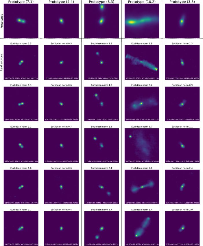
A89, page 7 of 22A&A 645, A89 (2021) Fig. 5. Closer look at five representative images with distinctly different shapes. The first row shows five hand-picked representative images from the trained SOM. The location of each representative image on the SOM is indicated by (column, row), thus the first highlighted representative image in this figure is positioned in the seventh column, second row of the SOM in Fig. 4. In each column, we show five (randomly selected) radio sources that have been mapped to the representative images in the first row. assigned to a representative image increases with the size and In Fig. 6, we label the SOM based on the category of known brightness of the representative image, as can be seen by compar- radio morphologies that each representative image most closely ing the radio sources associated with representative image (4, 4) resembles. Representative images that clearly belonged to more to those associated with representative image (10, 2): (10, 2) still than one group were assigned to multiple groups. They can be contains a variety of different morphologies whereas the sources seen to form fully connected groups (the map is cyclic) with the belonging to (4, 4) are all very similar. exception of two neurons labelled as “core-dominated doubles” A89, page 8 of 22
R. I. J. Mostert et al.: Unveiling radio morphology using self-organising maps

Fig. 6. Final 10 × 10 cyclic SOM manually labelled into seven categories. These categories describe the type of sources that are dominant or
most occurring in the set of sources that best matches each of the 100 representative images. If there are multiple dominant types of sources best
matching a representative image, the representative image is labelled using multiple categories, which is visualised by the dashed multi-coloured
edges.

and two neurons labelled as “Mix”, indicating that the topology           4.3. Morphology distribution of LoTSS extended radio
of the dataset is indeed conserved.                                            sources
    The labelling process reveals numerous distinct populations:
with “core-dominated” we indicate double-lobed AGN where                  In Fig. 7 we show the distribution of the number of best
the core has a higher peak flux than the lobes; “compact dou-             matching sources for each representative image in the SOM (a
bles” indicate compact, double-lobed AGN; “extended doubles”              “heatmap”). We can see that the most common representative
indicate double-lobed AGN where the hotspots are spatially                images are those that resemble unresolved sources or elongated
separated; “single lobe of extended doubles” indicate a (cata-            single sources while the least common represent faint sources
logue entry centred on a) single lobe of a double-lobed AGN.              with a hard-to-distinguish shape and core-dominated sources.
“elongated singles” indicate compact emission probably origi-                 After combining the heatmap with the representative image
nating from unresolved or barely resolved AGN or from strongly            labels assigned above, we get a picture of the overall morphology
beamed single AGN lobes. “(single lobe of) diffuse/large dou-             distribution of the extended sources in LoTSS DR1 (see Fig. 8).
bles” indicate either fluffy, double-lobed AGN or a single lobe           We caution however that these results serve as a first order esti-
of a large double-lobed AGN. Finally, “mix” is used for the two           mate and there will be individual sources best matching a given
SOM cells that contain a variety of sources (these often include          particular neuron that could be more accurately labelled by a
spurious emission from a neighbouring bright source).                     label not previously included.
    A distinct morphological population that is missing in these              If we count every source associated with the label “single
labels is that of bent FRI type sources. We expected that the dif-        lobe of an extended double” – disregarding the ones associated
ferent curvatures in the lobes of these sources results in them           to representative images with multiple labels and the ones asso-
ending up in various labelled groups within the SOM, not very             ciated to the label “(Single lobe of) large/diffuse doubles” – we
well represented by any of them. By mapping the NAT and WAT               can get a conservative estimate of the percentage of inadequate
collection from Mingo et al. (2019) to our SOM, we confirmed              source association by the source extraction software. As such,
that this is true. With a median value of 2.07, the Euclidean             we estimate that the percentage of inadequate source associ-
norm of the NAT and WAT sources to their representative image             ation for the 19 544 extended source entries in the catalogue
is 4% higher than that of the large non-bent FRI sources from             is about 13%. This percentage is higher than the percentage
Mingo et al. (2019) and 57% larger than the median Euclidean              of sources that were associated through visual inspection as
norm of all sources in our dataset, reinforcing our conclusion.           detailed by Williams et al. (2019): 5% of these 19 544 sources

                                                                                                                               A89, page 9 of 22
A&A 645, A89 (2021)
Euclidean norms
103 Median: 1.3
Number of radio-sources per bin
100 most Mean: 1.7
outlying objects Std. dev.: 1.4
Max.: 22.5(=17xmedian)
102
101
100
0 5 10 15 20
Euclidian norm to best matching prototype
Fig. 9. Histogram of the Euclidean norm from each radio source to its
closest representative image in the final 10 × 10 SOM, for each of the
19 544 radio sources in our final training set. Most sources have a very
small Euclidean norm to their best resembling representative image in
the SOM, which means they are morphologically similar to at least one
representative image in the SOM. We isolated the 100 most outlying
sources and show them in Appendix B.
Single lobe of
extended doubles
Compact doubles
103 Elongated
singles
Fig. 7. Heatmap of the 10 × 10 cyclic SOM, indicating the number of Extended doubles
(Single lobe of)
Number of sources
sources from our training dataset mapped to each of the representative large/diffuse doubles
images shown in Fig. 4. 102 Core-dominated doubles
Mix
101
100
0 5 10 15 20
Euclidean norm to best matching representative image
Fig. 10. Histogram of Euclidean norm from each radio source to its
closest representative image in the final 10 × 10 cyclic SOM, aggregated
by group. This shows how well each source resembles the best matching
representative image in its group. The lower the Euclidean norm, the
Fig. 8. Piechart of dominant groups in the 10 × 10 cyclic SOM, pro-
better the match. In general, a steeper declining trend indicates a better
viding a rough indication of the percentage of sources best matching a
match across sources with the same label.
neuron in each group. The number of sources best matching a neuron
that belonged to two groups was counted half for the tally in each group.
These are first-order estimates: each group will contain sources that a
human will classify differently after individual inspection. 4.4. Discovering morphologically rare sources through outlier
score
ended up combined in the value added catalogue8 . To per- The trained SOM gives us an overview of the archetypes or dom-
form this visual inspection and correct the PyBDSF catalogue inant morphologies present in the dataset. One can imagine that
Williams et al. (2019) use crowd-sourced manual component if the difference (the Euclidean norm) between a cutout and its
association through the Zooniverse platform9 . This platform best matching representative image is much larger than average,
allowed every source (LOFAR radio contours on top of a WISE see Fig. 9, this means that the cutout does not match well to
or Pan-STARRS image) to be viewed and associated by five dif- any representative image in the map. This implies that radio-
ferent astronomers. In the same process, optical and or infrared objects with this angular size and morphology are not abun-
host-galaxies were assigned to the radio emission if possible. dant in the training set: they are morphological outliers. The
Only associations agreed upon by four or five out of five peo- Euclidean norm between a cutout and its best matching repre-
ple were combined in the value added catalogue. The difference sentative image can therefore be seen as an “outlier score”.
between the number of source associations in Williams et al. Pre-processing the sources, specifically sigma-clipping or
(2019) and our estimate here shows the difficulty in distinguish- rescaling our cutouts, affects the magnitude of the Euclidean
ing between a pair of lobe-hotspots and two unrelated, unre- norm values. As we scale all our pixel values to range between
solved or barely resolved radio sources. 0 and 1, we are biased towards having large apparent objects
as outliers. For sources that are slightly different than their rep-
8
See the LoTSS-DR1 merged component catalogue: https:// resentative image, objects with a large angular size will have
lofar-surveys.org/public/LOFAR_HBA_T1_DR1_merge_ID_ a larger Euclidean norm than smaller sources. Indeed Fig. 10
v1.2.comp.fits shows that the group “(single lobe of) large/diffuse sources”
9
Web address: http://zooniverse.org shows higher Euclidean norms than all other groups. Before we
A89, page 10 of 22R. I. J. Mostert et al.: Unveiling radio morphology using self-organising maps
inspect the objects with high outlier score in our dataset, we dis-
cuss three options to reduce the bias in finding objects with large
angular size and explain why we do not use them.
The first option is scaling the pixel values such that the sum
of the pixel values add up to one in each cutout. This will steer
the bias towards sources that have bright emission concentrated
in a small area. In practice, cutouts with the highest outlier scores
will then be those compact bright doubles that enter the cat-
alogue slightly off-centre and compact objects with unrelated
neighbouring compact objects within our fixed-sized window.
A second option to reduce the bias is to look for the objects
with the highest Euclidean norm per labelled group of neurons.
As the groups represent sources of varying angular size, we can
expect to find outlying morphologies for sources with smaller
angular size. In practice, the objects with the highest Euclidean
norm in the groups – except in the “(single lobe of) large diffuse
doubles” group – are mostly artefacts and regular FRI or FRII
sources close to the noise-level. Visual inspection shows that
adopting a peak flux threshold of 0.5 mJy beam−1 and a total flux
threshold of 5 mJy, excludes most of the images containing these
artefacts. We then inspect the resulting 14 objects with the high-
est Euclidean norm per group in each of the groups except the
“(single lobe of) large diffuse doubles” group; these 84 sources
comprise 33 NAT or WAT objects, 42 non-bent FRI or FRII, and
9 sources too small or faint to clearly categorise. Many of the
non-bent FRI or FRII and a number of the other objects (31 out
of the 84 in total) received a high outlier score, not because of
their rare morphology, but because of unrelated close-by neigh-
bouring radio objects.
A third option to alleviate our bias towards finding outlier
objects with large angular size, is by including another mea-
sure in the outlier score. We experimented with an outlier score
that is the summation of the Euclidean norm and the Euclidean Fig. 11. Piechart showing the wide variety of morphologies and radio
norm times the fraction G times a tunable parameter γ. Here, G source types present in the 100 most outlying sources in the final
is the maximum sum of pixel values attained by any neuron in 10 × 10 cyclic SOM. Top panel: descriptive labels have been estab-
the SOM divided by the sum of the pixel values of the consid- lished by a manual visual inspection of each source in radio (LoTSS),
mid-infrared (WISE) and optical (SDSS9 colour). We labelled sources
ered neuron. Therefore, G will be one for the neuron with the
that fitted in more than one category as “ambiguous”. “X-type” sources
highest sum and proportionally bigger for neurons with smaller are “X-shaped” extended doubles (Rees 1978), “WATs” and “NATs”
summed values – thus proportionally bigger than one for neurons are Wide Angle Tailed and Narrow Angle Tailed sources, “WDS”
that represent sources with smaller angular sizes. By increasing are Wide Double Sources, “NEBD” are Narrow Edge Brightened
γ, we increase the outlier score for sources with smaller angu- Doubles (Miley 1980), “DDRG” are Double-Double Radio Galax-
lar sizes with respect to sources with larger angular sizes. This ies (Schoenmakers et al. 1999). An “AGN remnant candidate” is an
approach yields similar results to the previous experiment: we do extended double with such relaxed morphology that the AGN jets might
indeed find more small angular sized objects, but they are often not be active any more. As M101 is an exceptionally large apparent
positioned close to an unrelated neighbouring radio source. As object, the source detection software did not group the separate detec-
unrelated close neighbour sources do not represent physically tions of this nearby spiral, as a result it features multiple times in the cat-
alogue. Bottom panel: we grouped subtypes together to get an overview
rare objects, we do not consider this to be an optimal approach –
of the dominant types of sources in the outliers: “M101” was grouped
although ultimately the best definition to define outliers should with “nearby galaxy”; “complex” with “ambiguous”; “cluster relic”
depend on the user’s specific science goals. and “cluster halo” were grouped into “cluster emission” and “DDRG”,
In this paper, we use only the Euclidean norm as our out- “NEBD”, “NAT”, “WAT”, “WDS”, “double”, “asymmetric double” and
lier score and inspect the objects with the overall highest out- “X-type” were grouped into “AGN with jet activity”. A figure contain-
lier score. To illustrate the potential of this method, we select ing each of these one hundred most outlying sources can be found in
the 100 sources with the greatest outlier score (all sources to the Appendix B.
right of the red vertical line in Fig. 9) and present all of them in
Appendix B. To suppress the number of duplicate objects (broken
up during the automatic source-extraction) we require each table-
entry to be at a distance greater than 400 arcsec from all previ- motion through the circum galactic medium or rotation in the
ous table-entries. We visually inspected each of these 100 sources case of X-type sources (2%). Examples of outliers of each type
to investigate the nature of these outliers and provide a physical can be found in Fig. B.1 by looking at the Radio description
classification in Table B.1. In Fig. 11 we highlight the wide range in Table B.1. The sample is also diverse with respect to edge-
of different source-types and morphologies present. brightening and edge-darkening, we can see that the sample con-
We observe that 49% of the outliers are AGN with jet activ- tains 29 FRI and 25 FRII type sources. For three sources the
ity, the lobes thereof show a range of curvature – from wide FR classification is unclear and for the remaining sources it is
angle tailed (12%) to narrow angle tailed (2%) – indicating not applicable. The outliers cover multiple stages of jet-activity:
A89, page 11 of 22A&A 645, A89 (2021)
from active doubles, to “dying” AGN remnants, to restarted LoTSS-DR2 we find that 303 (30.3%) of the first 1000 outliers
Double-double radio galaxies. align with known SDSS galaxy clusters (Wen et al. 2012).
Although diverse, not all AGN that we present here can be The LoTSS-DR2 outlier source types include many AGN
regarded as radio objects with outlying morphologies. Specifi- with bent and or asymmetric jets, restarted AGN (DDRGs) and
cally, the Narrow edge brigthened sources, Wide double sources even phoenixes (revived fossil plasma in a galaxy cluster). A
and regular doubles account for 24% of the sources. These radio phoenix (source #181) features in Mandal et al. (2020); a
objects occur less frequently in the survey compared to simi- tailed AGN (source #320) features in Hardcastle et al. (2019);
lar objects of smaller angular size, but their morphologies can and a symmetric set of arcs around Abel 2626 (source #413) fea-
hardly be regarded as outlying. tures in Ignesti et al. (2017, 2018), Kadam et al. (2019), proving
Ten percent of the outliers are nearby starforming galax- that our method of finding morphological outliers is able to auto-
ies, where the radio-emission largely overlaps with the optical matically identify classes of rare sources with genuine scientific
emission in Pan-STARRS grizy bands. The synchrotron emis- importance.
sion originating from supernovas is a star-formation tracer that
is unobstructed by dust. As expected, both sharp cluster relics
like “bow shocks” and the more diffuse and amorphous cluster 5. Discussion
halos can also be found among the 100 objects with highest out- 5.1. Linear invariance and the challenge of radio source
lier scores. association
Twenty-three percent of the outliers are ambiguous or com-
plex in nature. Most ambiguous outliers (16%) are diffuse and Without correctly associated radio sources and corresponding
somewhat amorphous, raising the question whether they are correct apparent size estimates, we are not able to linearly rescale
active AGN, AGN remnants or cluster related emission. For the each radio source in size to make the SOM linearly size invari-
complex objects (7%), there seems to be additional interaction ant. This means that objects that appear to be large on the sky
with neighbouring objects. will also appear as larger shapes in the SOM.
In Fig. 12, we highlight a number of individual outliers. The Given a large enough SOM, some neurons will start to repre-
red boxes within these images show the fixed size of the cutouts sent parts of larger objects such as a single lobe of an AGN with
as they enter the SOM for training: the solid red boxes show the large angular size. In practice, these neurons may also resemble
initial 142.5 × 142.5 arcsec2 cutout and the inner (dashed) boxes the disk-shaped emission of a nearby starforming galaxy, limit-
show the 100 × 100 arcsec2 cutout after cropping as described in ing the SOM’s ability to separate intrinsically different sources.
Sect. 3.2. The figure shows that objects that fall entirely within Sources much smaller than our fixed image size of 100 arcsec
the fixed-size box, and those which extend beyond it, can both with closeby (within 50 arcsec) neighbouring sources are also
be given high outlier scores, demonstrating that the fixed cutout poorly analysed by our method. Indeed, inspection of the out-
size does not prevent us from finding morphological outliers of lying objects per group shows that many images with a high
different apparent sizes, even when relying on imperfect source Euclidean norm are often occurring morphologies like regular
extraction. compact FRII with closeby unrelated radio sources. The group
It is possible to map a dataset to an SOM that is trained on of neurons labelled as “(single lobe of) large diffuse doubles” are
a similar dataset. We can thus quickly find outliers in a newly the exception to this observation.
observed parts of the sky within the same survey. We showcase At this moment, no automatic source extraction code comes
this concept by looking for outliers in a new dataset covering close to a human ability to associate spatially separated radio
5296 (5720 − 424; LoTSS-DR2 minus the LoTSS-DR1 area) emission. However, source association performed by humans is
square degrees. To avoid distortion by the synthesised beam, we a tedious, time intensive process.
used all objects within a radius of 2.5 degree around the centre of An ongoing LOFAR Galaxy Zoo project tackles the associa-
each field. Analogous to the approach for LoTSS-DR1, we sup- tion problem for LoTSS-DR1 (Williams et al. 2019) and LoTSS-
press the number of duplicate objects by imposing a minimum DR2 and can thereafter serve as labelled training sample for
separation distance of 200 arcsec between the listed outliers. supervised learning attempts to the radio component associa-
Table 2 shows an excerpt of the table of the 1000 most out- tion problem. Dieleman et al. (2015) and Dai & Tong (2018)
lying objects in this dataset. Again, the outliers include objects were successfully able to recreate the labels assigned to galax-
that span a large range in apparent size and morphology. The ies by volunteers in the Optical and Radio Galaxy Zoo projects
apparent sizes range from less than a hundred arcsec to a degree. respectively. Wu et al. (2019) use FIRST and WISE images
The morphologies include soft-edged (diffuse) emission as well combined with Radio Galaxy Zoo crowd-sourced associations
as sharp-edged (compact) emission. Cross-matching against the (Banfield et al. 2015) to combine radio blob detection, associa-
extended source catalogue (2MASX; Jarrett et al. 2000) from the tion and classification using a promising deep learning approach.
Two Micron All Sky Survey (2MASS; Skrutskie et al. 2006), we In this paper we showed that it is possible to select morpho-
see that 93 (9.3%) of the first 1000 outliers align with a 2MASX logically rare objects in large datasets with no previous human
object (with radius >15 arcsec), indicating that the outliers con- created labels or associations. Our selection works across a range
tain numerous nearby starforming galaxies. of apparent sizes and for broken up sources. We did not find an
In Fig. 11 we see that for the 100 outliers of LoTSS-DR1, upper limit to the angular size of objects for our ability to mark
based on their radio morphology, a significant percentage can be them as having a rare morphology. However, we can conclude that
classed as cluster emission (either as relic or halo emission). Fur- our SOM approach to finding outliers is ill-suited to find sources
thermore, the movement of the AGN in the intra-cluster medium with outlying morphologies with angular sizes much smaller
is known to effect the morphology of AGN radio emission and than our fixed view window. Specifically using the Euclidean
can for example lead to long bent tails. As such, many of the norm as outlier score and a fixed view window of 100 arcsec,
WAT identified by the outlier selection will likely also be asso- we find no sources with an angular size smaller than 45 arcsec
ciated with galaxy cluster or group environments. Indeed for in our list of 100 outliers (Appendix B).
A89, page 12 of 22You can also read