Learning autonomous maritime navigation with offline reinforcement learning and marine traffic data

Åbo Akademi

 Learning autonomous maritime
navigation with offline reinforcement
 learning and marine traffic data

 Jimmy Westerlund 39053

 Master’s thesis in Computer Engineering

 Supervisors: Sebastien Lafond & Sepinoud Azimi
 Rashti

 Åbo Akademi University

 Faculty of Science and Engineering

 Information Technologies

 2021

Abstract
Autonomous shipping is a heavily researched topic, and currently, there are large amounts of
ship traffic data available but unexploited. Autonomous ships have the potential to reduce costs
and increase safety. The challenge is achieving the correct maritime navigation behavior
according to the situation reliably, which may be possible by exploiting historical ship traffic
data. This thesis explores the possibility of using offline reinforcement learning based on AIS
data to learn autonomous maritime navigation.
The hypothesis that AIS data can be used for training a reinforcement learning agent is tested
by implementing an offline reinforcement learning agent. For comparison, an online agent that
learns without data is also implemented. Both agents are trained and evaluated in a simulator,
and the goal of both agents is to learn to navigate to a destination, given a starting point.

The results suggest that offline reinforcement learning can be used for automating maritime
navigation, but a more extensive and more diverse dataset is needed to conclude its
effectiveness.

Keywords: Reinforcement learning, offline reinforcement learning, autonomous navigation,
autonomous ship, AIS

Preface
I want to say a special thanks to my supervisors Sepinoud and Sebastien, for their guidance and
motivation throughout the project. Also, thanks to Richard Nyberg for helping me get started
with the project and explaining how to use the simulator.

Table of Contents
1. Introduction ............................................................................................................................ 1

2. Reinforcement learning.......................................................................................................... 3

 2.1 History .............................................................................................................................. 3

 2.2 Markov Decision Process ................................................................................................. 5

 2.3 Elements of reinforcement learning ................................................................................. 6

 2.3.1 Agent and Environment ............................................................................................. 6

 2.3.2 Policy ......................................................................................................................... 7

 2.3.3 Reward function ........................................................................................................ 8

 2.3.4 Value functions .......................................................................................................... 9

 2.3.5 Model ....................................................................................................................... 11

 2.4 Offline reinforcement learning ....................................................................................... 11

 2.5 Algorithms...................................................................................................................... 12

 2.5.1 Q Learning ............................................................................................................... 13

 2.5.2 Deep Q-learning ...................................................................................................... 14

3. The project ........................................................................................................................... 16

 3.1 Goal ................................................................................................................................ 16

 3.2 The dataset...................................................................................................................... 17

 3.3 Ship terminologies.......................................................................................................... 18

 3.4 The ship simulator .......................................................................................................... 19

4. Implementation .................................................................................................................... 21

 4.1 Libraries ......................................................................................................................... 21

 4.1.1 TensorFlow .............................................................................................................. 21

 4.1.2 Keras and Keras-rl ................................................................................................... 22

 4.1.3 PyTorch ................................................................................................................... 22

 4.1.4 d3rlpy ....................................................................................................................... 23

 4.1.5 NumPy ..................................................................................................................... 23

4.1.6 Pandas ...................................................................................................................... 23

 4.1.7 Gym ......................................................................................................................... 24

 4.2 Setting up a scenario ...................................................................................................... 24

 4.3 Online agent design ........................................................................................................ 25

 4.4 Offline agent design ....................................................................................................... 29

 4.5 Changes during implementation..................................................................................... 33

5. Results .................................................................................................................................. 34

 5.1 Online agent ................................................................................................................... 34

 5.2 Offline agent................................................................................................................... 36

6. Discussion ............................................................................................................................ 40

7. Future work .......................................................................................................................... 42

 7.1 Online agent ................................................................................................................... 42

 7.2 Offline agent................................................................................................................... 44

 7.3 General ........................................................................................................................... 46

8. Conclusion ........................................................................................................................... 47

9. Swedish summary ................................................................................................................ 48

 9.1 Introduktion .................................................................................................................... 48

 9.2 Förstärkt inlärning .......................................................................................................... 49

 9.3 Projekt ............................................................................................................................ 50

 9.4 Implementation............................................................................................................... 50

 9.5 Resultat ........................................................................................................................... 51

 9.6 Slutsats ........................................................................................................................... 52

References ................................................................................................................................ 53

1. Introduction
Over the past decade, there has been a dramatic development in the field of autonomous
technologies. Autonomous systems are being applied in transportation systems, and with the
technological breakthrough, the reality of fully autonomous transport systems may not be so
distant. Giants like Google and Tesla are two leading developers of fully self-driving systems
for road transport, and their partially self-driving systems are already available in many new
cars [23]. For air-based transport, uncrewed aerial vehicles (UAVs) are being used for delivery
services. In Helsinki, for example, a delivery system using drones is being developed by Wing
[24]. Maritime transport is the sector responsible for the majority of all transport. Among the
leading developers of autonomous maritime systems are Rolls-Royce and Kongsberg, but no
fully autonomous vessels are used commercially yet. Autonomous maritime navigation is an
area of broad and current interest, and it is also the topic of this thesis.

A study in the report Review of Maritime Transport 2020 [25] shows that over 80 percent of
global trade by volume is carried out by cargo ships. Moreover, shipping is the only viable
option for international trade, as it is by far the most cost-effective option for transporting large
volumes of merchandise [26]. However, the shipping industry faces immense economic,
environmental, and safety challenges as traditional solutions, such as building larger and more
optimized ships, reach their limits.

It is estimated that over 75 percent of maritime accidents involve human error [27].
Furthermore, an analysis of around 15 000 maritime liability insurance claims between 2011
and 2016 was done by Allianz Global Corporate & Specialty (AGCS) and concluded that
human error was a primary factor in 75% of all cases, equivalent to 1.6 billion dollars in losses
[27].

Crewless autonomous ship systems would enable new ship designs, as the bridge and the living
spaces on vessels could be removed to improve aerodynamics and reduce fuel consumption. It
would also lower crew costs and ultimately improve safety by removing the human element.
Autonomous ships are believed to be a potential solution to the difficulties the shipping
industry faces, offering safer and more cost-effective shipping [26].

Reinforcement learning used for autonomous driving and navigation is a reasonably new
approach. Even more recent is the idea of using data-driven reinforcement learning in maritime
navigation, which is enabled by the collection of automatic identification system (AIS) data.

 1

According to Regulation 19, all cargo ships weighing over 500 tons and all passenger ships,
irrespective of size, must be fitted with AIS [28]. The AIS data contains information about the
vessel, such as the coordinates, speed, and heading. AIS data contains valuable information
that can, in theory, be used to learn autonomous maritime navigation. This thesis studies the
possibility of using offline reinforcement learning with AIS data to learn autonomous maritime
navigation.

 2

2. Reinforcement learning
Reinforcement learning (RL) is the approach of computationally automating tasks by
specifying a goal and a set of rules to follow. What sets reinforcement learning apart from other
machine learning approaches is that the RL agent interacts directly with the environment and
learns to make decisions based on direct feedback from the environment [1]. Compared to
supervised learning, the strength of reinforcement learning lies in the lack of need of data. In
supervised learning, labeled data is used to learn a specific behavior. The data contains
information about what the correct action in a particular situation would be [1]. This approach
can yield successful results in cases where large amounts of data are available. Still, in
unexplored or partially unexplored environments with limited or no data available,
reinforcement learning is more applicable. However, there are also hybrid approaches;
recently, the interest in data-based reinforcement learning, also known as offline reinforcement
learning, has grown as it has shown great potential in solving various problems [5].

Navigating a ship from a starting point to a destination can be defined as a problem with a goal,
a set of possible actions, and a set of rules that the ship must follow while maneuvering its way
to the destination. With this definition, it can be thought of as a problem that can be solved
with reinforcement learning. The problem is, of course, more complex in reality, but the
essential idea of RL can be explained through this simple example. Maritime navigation with
reinforcement learning is the core of this thesis, and the possible actions, rules, and goal of the
thesis will be discussed in greater detail in the next chapter. In contrast, this chapter will review
the general history and elements of reinforcement learning.

2.1 History
In the book Reinforcement Learning: An Introduction, Sutton and Barton explain that modern
reinforcement learning has its roots mainly in two different methods, namely learning by trial-
and-error and optimal control [1]. The methods evolved independently and eventually
intertwined in the early 1980s to form what is known as reinforcement learning today.

Learning by trial-and-error stems from psychological studies of animal learning and is
generally regarded as the earliest studies in artificial intelligence [1]. The idea dates back to the
late 1800s when the British psychologist Conway Lloyd Morgan used the term “trial-and-error
learning” to describe animal behavior. In the early 1900s, American psychologist Edward Lee
Thorndike formulated a principle about trial-and-error learning, known as the “Law of Effect”

 3

principle, which involved positive reinforcement and negative reinforcement. According to
Sutton et al., Alan Turing was among the first to approach the idea of implementing trial-and-
error learning in a computer [1]. In 1948, Turing wrote a report about a “pleasure-and-pain
system” based on Thorndike’s “Law of Effect” principle. In the report, Turing describes a
system that would take an action randomly and save the results temporarily. When a negative
reinforcement occurs, the system will discard all temporarily saved results, and when a positive
reinforcement occurs, it will save the results permanently [1].

Optimal control is a term that emerged in the 1950s and it describes the method of designing
controllers for dynamical systems [1]. Richard Bellman developed a proposed solution to
optimal control. The proposed solution uses a value function and the states of a dynamical
system to define a function that became known as the Bellman equation [1]. The methods that
solve this equation are categorized as dynamic programming.

Dynamic programming is the methodology of breaking down a complex problem into smaller
subproblems and solving them individually before combining them into a final solution [2]. A
dynamic programming algorithm saves the answers to all solved subproblems in tables [2]. The
algorithm will only have to calculate the answers to the subproblems once, as the answers can
be fetched directly from the table in case the subproblem needs to be solved again. However,
one of the most significant drawbacks with dynamic programming is that its computational
needs grow exponentially with the complexity of the problem since the number of subproblems
grows with the number of state variables [1].

In the early 1960s, the research in artificial intelligence shifted from reinforcement learning to
supervised learning, and the distinction between the two types was often confused [1].
Following the confusion, research in reinforcement learning stagnated in the 1960s and early
1970s, but in the mid-1970s, Harry Klopf recognized that the adaptive behavior in artificial
intelligence was fading due to most researchers focusing on supervised learning. Through this
realization, Klopf linked trial-and-error learning to reinforcement learning again and made a
clear distinction between reinforcement learning and supervised learning [1].

Apart from dynamic programming, two other reinforcement learning methods are commonly
used, namely Monte Carlo (MC) methods and temporal difference (TD) learning. Unlike
dynamic programming, Monte Carlo methods do not require a complete model of the
environment, but their downside is that they update the policy only after an episode has
terminated, not at every time step [1]. As stated by Sutton et al., MC methods are a way of

 4

solving RL problems by averaging sample returns, and this approach is only suitable for
episodic tasks. Lastly, TD learning methods combine the strengths found in DP and MC
methods [1]. TD methods learn from experience without a model, and they can also make
predictions mid-training, as the policy is updated at each time step.

2.2 Markov Decision Process
Before delving into the elements of reinforcement learning, it is important to first explain the
core mathematics behind reinforcement learning, namely the Markov Decision Process (MDP).
In case the state and action space of the MDP is finite, it is called a finite Markov Decision
Process (finite MDP) [1]. According to Sutton et al., finite MDP is a vital part of reinforcement
learning. They state that a large amount of modern reinforcement learning can be understood
simply by understanding MDPs.

To express a reinforcement learning task as an MDP, it must first fulfill the requirement of the
Markovian property [1]. A task is said to have the Markov property if the next state ′ at time
 + 1 only depends on the state and action , at time . A task with the Markov property is
called an MDP, and it enables the predictions of the following state and the expected next
reward, given the current state and action [1]. With a given state and action the probability
of every next state ′ and reward is expressed with the following formula [1]:

 ( ′, | , ) = Pr{ +1 = ′, +1 = | = , = }

This formula fully expresses the dynamics of a finite MDP, and it enables the computation of
other things regarding the interaction between the agent and the environment. An example is
the formula for calculating the state-transition probability, which gives the probability of
transitioning to state ′, given a state and an action [1]:

 ( ′| , ) = Pr{ +1 = ′ | = , = }

 5

An MDP is represented as a 5-tuple [1][3]: ( , , , , ) where:

 • – a finite set of states
 • – a finite set of actions
 • – a set of state-transition probabilities
 • ( , ′ ) – the immediate reward distributed by a reward function when transitioning
 from state to state ′ through action 
 • ∈ [0, 1] – the discount rate

To clarify, a set of states are values that describe the situation the agent is in, and a set of actions
describes what actions the agent performs. The discount factor is a value between 0 and 1 which
determines the current value of future rewards, as discussed further in this chapter.

2.3 Elements of reinforcement learning
According to [1], reinforcement learning is defined by the following elements: agent,
environment, policy, reward function, value function, and model. These are the building blocks
that define what reinforcement learning is, and they are explained in greater detail in the
following sections.

2.3.1 Agent and Environment
In reinforcement learning, the two first elements are the agent and the environment. The
learner, which is also the decision-maker, is called the agent [1]. What it interacts
with, containing everything outside the agent, is called the environment. State and action are
two terms used to describe what situation the agent is currently in. A state contains information
about where in the environment the agent is at a given moment, and the action describes what
action the agent takes. The agent and the environment are connected through their interactions;
the agent takes an action, and the environment reacts to the action by presenting a new state to
the agent. The interaction between the agent and the environment occurs at each time step,
where the discrete time step is a sequence [1]: = 0, 1, 2, 3, … As stated by Sutton et al., time
steps can also be continuous, though continuous time steps involve more complex calculations
compared to discrete time steps. In this thesis, only discrete time steps are considered as they
are simpler to deal with, and it applies well to ship log files, where each row in the data

 6

corresponds to 1 second. The use of discrete time steps will be more explicit in the next chapter,
where the ship log files from Aboa Mare are explained in further detail.

Figure 1 is a visualization by Sutton et al., and it is widely used to illustrate the interaction
between the agent and the environment. The agent starts in time step t and takes an action 
based on the initial state and reward . The environment responds to the action by providing
the agent with a new state +1 and a new reward +1 and the interaction continues. The
environment generates rewards that the agent tries to maximize over time. In some cases, it can
be difficult to define the boundary between agent and environment, but the general rule is that
anything that the agent cannot change is considered outside of it and thus part of its
environment. In the case of an autonomous ship, the ship is the agent, and everything else,
such as the water, the land, and the sea marks combined, make up the environment.

Figure 1: Agent and environment interaction visualized by Sutton et al. [1]

2.3.2 Policy
The policy defines the agent’s behavior in any state; in other words, the policy is the agent’s
strategy. It is a mapping from each state and action in the environment to the probability of
taking a specific action when being in a particular state [1]. The policy is an essential part of a
reinforcement learning agent, as it alone is enough to define the behavior of the agent.
Essentially, solving a reinforcement learning task is to find the policy that brings the largest
number of rewards over a long time. As stated by Sutton et al., this policy is called the optimal
policy [1].

 7

Reinforcement learning methods are usually categorized as being either on-policy or off-policy,
depending on how the agent achieves the optimal policy [1]. In on-policy methods, the agent
learns how good actions are based on a specific policy by observing the rewards generated
when following that policy. In off-policy methods, the agent learns how good actions are based
on a behavior policy 1 by observing the rewards generated when following a different policy
 2 called the target policy.

2.3.3 Reward function
A reward in reinforcement learning is a numeric value that the agent receives at each time step
of the training, and it is also what defines the goal of a reinforcement learning problem [1]. The
objective of the reinforcement learning agent is to maximize the total reward over a longer
time. The reward function defines what behavior should be rewarded and what behavior should
be punished. With a well-made reward function, the agent will thus be able to learn the desired
behavior. The reward is also a deciding factor for altering the policy since the agent will
recognize that an action followed by a low reward may not be optimal. As a result, the policy
might change to make the agent take a different action if faced with the same situation in the
future [1].

In some reinforcement learning scenarios, the interaction between the agent and the
environment naturally breaks up into segments. These segments are called episodes and what
divides one episode from another is a reset of the environment. In the example earlier described
where an agent must learn to navigate a ship from a starting point to a destination, an episode
would end if the agent reached the goal, but it would also end if the agent did not reach the
destination within a specific time limit, in case there was a time limit defined. Every episode
ends with a state called the terminal state, which is always followed by resetting the
environment to a default starting state [1].

The expected return is the total amount of rewards that the agent is expected to gather, and for
the most straightforward cases, it can be expressed as the sum of the rewards [1]:

 = +1 + +2 + +3 + ⋯ + 

 8

where is the reward in time step and is the last time step. To avoid dealing with infinite
rewards, the formula can be further developed by introducing a discount rate , a value within
the bounds of 0 ≤ ≤ 1. The discount rate tells the current value of future rewards, which
helps the agent choose between immediate and future rewards [1]. A discount rate of 0 will
result in the agent prioritizing to maximize the immediate rewards from the next time step, but
when the discount rate approaches 1, the agent will also take future rewards into account [1].
Without a discount rate, the agent is at risk of getting stuck doing the same actions repeatedly
but never reaching the goal. The discounted return is represented by [1]:

 ∞

 = +1 + +2 + +3 + ⋯ = ∑ + +1
 2

 =0

The formula says that a reward received time steps into the future is only worth −1 times
what it would be worth immediately [1].

Like several other aspects of reinforcement learning, the idea of discounting is also based on
human psychology. As presented by Leonard Green and Joel Myerson [4], an example of
human discounting is when faced with the option of receiving 100€ now or 120€ in a month,
the immediate reward might seem more appealing. However, if both rewards are shifted one
year into the future, the choice is to receive 100€ in one year or 120€ in 13 months. The larger
reward suddenly seems like the obvious choice, as the sooner reward has become discounted
because it is so far in the future.

2.3.4 Value functions
Closely related to the reward function are the value functions. While the reward function
defines what action yields the best reward in the current state, the value functions specify what
actions are best for collecting the most rewards over a longer time. The value of a state is the
total amount of rewards an agent can be expected to collect in the future, given a starting state
 and a policy . This value is calculated through the state-value function and is expressed as
[1]:

 9

∞

 ( ) = [ | = ] = [∑ + +1 | = ]
 =0

where is the expected value, is the discounted return and is any time step. Another
value function is the action-value function, which gives the value of taking an action in state
 with a policy [1]:

 ∞

 ( , ) = [ | = , = ] = [∑ + +1 | = , = ]
 =0

The value functions and are needed because states that yield low immediate rewards
might lead to states with high rewards. The reverse can also be true; states which produce high
immediate rewards might lead to states with low or even negative rewards.

The state-value function can be used to derive the formula called the Bellman equation [1]:

 ( ) = ∑ ( | ) ∑ ( ′, | , )[ + ( ′)]
 ′ , 

The Bellman equation expresses the relation between the value of a state and the value of future
states. Essentially, it is the product of the sums of two probabilities. The first, ( | ), is the
probability of taking action in state while following policy and as earlier discussed,
 ( ′, | , ) is the probability of ending up in a state ′ with reward while being in state 
and taking action . The value is calculated with the sum over the values of the actions ,
future state ′ and reward . For each , ′ , the probability ( | ) ( ′ , | , ) is calculated
and weighted by the quantity [ + ( ′)]. Finally, the expected value is given by the sum of
all possibilities [1].

 10

2.3.5 Model
The model is the sixth and final element of some, but not all, reinforcement learning systems.
As the name indicates, it is a model of the environment, and it can be used in various ways to
enhance an RL system. For example, with the input of a state and an action, the model can
predict what the next state and next reward will be [1]. A model enables planning, meaning
that we can decide what actions to take by considering future situations. Reinforcement
learning methods utilizing a model are called model-based, while the methods purely built on
trial-and-error style learning are called model-free [1].

2.4 Offline reinforcement learning
Reinforcement learning methods that utilize previously collected datasets for training without
interaction with an environment are categorized as offline reinforcement learning [5]. Offline
reinforcement learning algorithms have shown great promise in teaching optimal decision-
making based on large datasets. In this section, the main goal is to explain the core idea of
offline reinforcement learning and the benefits and drawbacks.

In traditional reinforcement learning, also known as online reinforcement learning, the agent
explores the environment and learns by trial and error. This is not an issue with small, simple
tasks that can easily be simulated, but a problem arises when dealing with large and complex
tasks with no access to a realistic simulated environment in which the online agent can be
trained. Building simulated environments for autonomous driving and healthcare tasks, for
example, can be both expensive and dangerous. The challenge lies in building accurately
simulated environments for the agents to train in, as the tasks can be complex and very different
from each other. Furthermore, there is always a risk of error when transferring an agent from
training in a simulated environment to solving real-world tasks.

In offline reinforcement learning, the agent does not have to interact with the environment, and
instead of exploring the environment, it must exploit the dataset. With a large enough dataset,
the idea is that the agent will be able to learn the optimal policy both reliably and quickly. The
algorithm is given a static dataset of transitions = {( , , +1 , )} and must try to learn the
optimal policy based on it [5]. Ultimately, the goal of offline reinforcement learning is to find
the optimal policy that performs better than the behavior observed in dataset .

 11

The great benefit of a successful offline reinforcement learning implementation is the lack of
need for a simulated environment, in addition to the possibility to learn based on previously
collected data. An added benefit is not having to address the exploration-exploitation trade-
off. This is the dilemma of choosing between exploring new actions or exploiting known actions
[1]. The agent must exploit known action to collect rewards, but it must also explore new action
to make more optimal choices in the future. When learning based on a static dataset, the agent
can only exploit the transitions found in the dataset.

However, there are a couple of issues as well that need to be considered. One of the biggest
challenges in offline reinforcement learning is the fact that the training relies solely on the
transitions in the dataset. This means that the agent will not be able to explore the environment
to learn possible high-reward regions that exist outside of the dataset [5]. Another issue is the
amount of data required to train an offline reinforcement agent. It is impossible to say an exact
amount of data required for successful training as it depends on the complexity of the problem
and the complexity of the algorithm, but generally, a larger dataset gives the potential for more
successful results. With a small dataset, there is a risk that the agent is never able to find an
optimal policy [5].

2.5 Algorithms
Essentially all reinforcement learning algorithms implement the same learning loop: the agent
interacts with the environment while following a behavior policy. The agent observes the state,
picks an action, observes the next state and the reward. This loop may repeat multiple times,
and the policy is updated using the observed transitions [5].

There are many well-built algorithms for solving reinforcement learning problems, and
choosing which one to use is not necessarily straightforward. In this thesis, the Deep Q-
Network algorithm is used because it is a well-known algorithm. It has successfully been
applied to solve tasks in simplified environments with discrete action spaces, such as vehicle
navigation among pedestrians [8] and path planning of ships [9]. Additionally, several libraries
with the Deep Q-Network algorithm implemented are available, which further speed up the
development process.

 12

2.5.1 Q Learning
Many new algorithms have emerged throughout the years, and most are improved versions of
older ideas and approaches. Q-learning is regarded as one of the most important breakthroughs
in the history of reinforcement learning, and it is the base of several modern algorithms [1].

In 1989, Anthony Watkins presented Q-learning, which is a model-free reinforcement learning
algorithm based on dynamic programming methods [6]. It enables the agent to learn by
evaluating the consequences of its actions in the environment. The agent tries all possible
actions in all possible states and learns which actions are best based on the discounted return
[1][6]. As stated by Watkins and Dayan [6], the object in Q-learning is to estimate the Q-values
for an optimal policy. If the agent can successfully learn the Q-values, it can also decide the
optimal actions in states. The Q-values are given by the Q-function ( , ), which is
equivalent to the action-value function earlier discussed. Each calculated Q-value is updated in
a look-up table used in future calculations [6]. The Q-learning algorithm is represented by [1]:

 ( , ) ⟵ ( , ) + [ +1 + max ( +1 , ) − ( , )]
 
As seen in the formula, the Q-value, which is updated each time step, is the sum of three factors:

 • ( , ) + : The current Q-value weighted by the learning rate
 • +1 : The reward in the next time step, weighted by the learning rate
 • max ( +1 , ): The action with the highest estimated action value based on all
 
 possible actions in the following state

The learning rate 0 ≤ ≤ 1 determines at what rate the agent should overwrite previously
learned behavior; in other words, it determines how quickly the agent should learn a behavior.
A value of 0 will make the agent learn nothing, while a value of 1 makes the agent overwrite
all previously learned information on each time step [1].

 13

2.5.2 Deep Q-learning
Q-learning’s main problem is that the look-up table also quickly grows in size in tasks
involving many states and actions. Additionally, to accurately estimate the value of an action,
the agent must explore every state in the environment, which is unrealistic for larger
environments. As an answer to these problems, Minh et al. propose the Deep Q-Network
(DQN) in the research paper Human-level control through deep reinforcement learning,
published in 2015 [7]. The proposed algorithm is a combination of Q-learning and deep neural
networks, and its advantage over Q-learning is the ability to approximate the optimal action-
value function using a deep convolutional neural network instead of a look-up table [7]. With
DQN being able to approximate the action-value function, it is more effective than Q-learning
in tasks involving large state- and action spaces.

A deep convolutional neural network (DCNN) is a type of feed-forward neural network (FNN)
[9], illustrated in Figure 2. A neural network of this kind works by distributing the input to the
hidden layers, which will make decisions from previous layers and weigh whether a stochastic
change within itself will be good or bad for the final output [9]. A neural network becomes a
deep neural network when the architecture contains multiple hidden layers.

Figure 2: A three-layered feed-forward neural network (FNN), comprised of an input layer, a hidden layer, and an output
layer.

 14

Reinforcement learning methods are notoriously unstable when neural networks approximate
the action value [7]. According to Minh et al., the reason behind the instability is caused by
two things. Firstly, due to minor updates to Q may significantly change the policy, and
secondly, due to the correlations between the action-values and the target values. To stabilize
the learning, Minh et al. introduce experience replay and a target network [7].

Experience replay is the method of storing an agent’s experience into a replay memory, and at
each time step, the replay memory is updated. During the training, random samples from the
replay memory are picked out and used for training the agent [7]. Experience replay improves
training because it breaks the correlation between consecutive samples. Furthermore, it
smoothes out learning and avoids oscillations because the behavior is averaged over past
experiences. To further improve the stability of Q-learning, a target network is introduced. At
a set interval, the network is cloned to obtain a target network, which is used for computing the
estimated Q-values.

 15

3. The project
The idea for this thesis project came from The Institute of Maritime Software Technology
(MAST! Institute), a collaboration between Åbo Akademi University and Novia University of
Applied Sciences. Research projects in the MAST! Institute focus on maritime digitalization
and autonomous ships. With a combination of software expertise from Åbo Akademi
University and the tools and knowledge at Novia’s Maritime Academy, Aboa Mare, the goal
is for the MAST! Institute to contribute to maritime research and develop new solutions for
autonomous shipping [10].

The implementation and the testing of reinforcement agents are done in the Simple Ship
Simulator, a ship simulator developed by Ivan Porres, Kim Hupponen [11], and Sebastian
Penttinen [12]. The simulator was built for evaluating machine learning algorithms for
autonomous ships.

3.1 Goal
This thesis explores the possibility of training an offline reinforcement learning agent based on
previously collected ship data. The ship log data were collected from the simulator at Aboa
Mare. The collection process was part of two other master’s theses projects done by Richard
Nyberg and Tatjana Cucic.

Evaluating an offline agent’s performance can be difficult, and as a means of comparison, an
online agent was developed alongside the offline agent. The online agent enables comparing
performance and training times between the two agents, which can help make a final verdict
about the offline RL agent’s performance. Both agents are tested in the Simple Ship Simulator,
where they are faced with solving the same seemingly simple task: navigate to a destination,
given a starting point. The ultimate goal is for both agents to learn to solve the task successfully,
followed by analyzing the data logged during training to reach a conclusion about offline
reinforcement learning used in autonomous maritime navigation.

 16

3.2 The dataset
The dataset contains ship traffic data collected from a realistic simulator during the training of
students at Aboa Mare. In its raw format, the data came in Automatic Identification System
(AIS) format encoded by the National Marine Electronics Association (NMEA) standard.
Richard Nyberg and Tatjana Cucic extracted the raw data from the simulator at Aboa Mare and
converted it into Comma Separated Value (CSV) files. Compared to raw data, CSV files are
much easier to work with as they contain distinct rows and columns with informative headers.
CSV files can also be visually inspected in Microsoft Excel, as it is a supported file format.
The CSV files are referred to as “the dataset,” and they are the starting point of the offline
reinforcement learning agent.

Before preprocessing, the dataset contains 54 columns of parameters that hold information
about the ship, such as the location, the speed, the direction, and the weather. However, only a
fraction of the parameters are relevant for a proof-of-concept offline reinforcement agent, and
the data preprocessing is discussed in the next chapter. Each CSV file holds information about
the trajectory of one ship. Each row in the files corresponds to a second, and the state space is
naturally discretized into one-second time steps. The dataset contains recorded behavior from
four different areas: The North Sea, the Channel to Felixstowe, Dover Strait, and Rotterdam.
The traffic recorded in the Rotterdam area was selected as the best of these locations, because
it contained the most concentrated coordinates. The traffic in the Rotterdam area involves
simulation data from 102 separate ships. Importing the data from the Rotterdam area into a
GPS visualizing tool [14] generated Figure 3. The tool draws a red dot on a nautical map for
each coordinate contained in the dataset. As seen in the figure, the traffic is heavily
concentrated in a specific area, which is beneficial, given the small dataset. An offline
reinforcement learning agent with a starting point and a destination within the area of
concentrated data points should have a good chance of learning to navigate to the destination
successfully.

 17

Figure 3: Data points from 102 separate ship simulation runs imported into a GPS visualizing tool [14].

A critical remark about the dataset is that it is recorded human behavior, which means that it
may contain non-optimal behavior or errors that can affect the agent’s learning. For this thesis,
though, the quality of the data is not considered.

3.3 Ship terminologies
The names of the parameters in the dataset are not self-explanatory. Therefore, a subchapter
explaining the relevant parameters and ship terminologies related to the parameters is
necessary. A ship is affected by several external forces, which also affect the route it travels.
The term “heading” is used to express the direction a ship is pointing. Still, because the ship
can drift sideways due to environmental factors, such as the wind and the current, the term
Course over Ground (COG) is used to express the ship’s trajectory accurately. COG is the
direction the boat travels relative to the bottom [13]. Similarly, Speed over Ground (SOG) tells
the vessel’s true speed, as it expresses the ship’s relative to the ground.

The motion of a ship is expressed through six terms: surge, sway, yaw, heave, pitch, and roll.
The SSS supports surge, sway, and yaw. For further simplification purposes, only surge and
yaw are used in this implementation. Surge expresses the forward and backward movement of
a ship, which is controlled by the throttle. Yaw describes the side-to-side movement of the stern
and bow and is controlled by the rudder angle.

 18

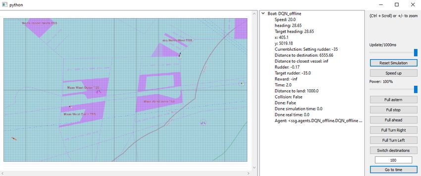
3.4 The ship simulator
The Simple Ship Simulator (SSS) is strictly software-based and must not be confused with
Aboa Mare’s simulator. Though the simulator at Aboa Mare is realistic and sophisticated, it is
not well suited for testing and deploying custom machine learning solutions. SSS was
developed to enable quick development and evaluation of machine learning algorithms of
autonomous ships. The simulator is roughly divided into seven parts: the agent, the gym
environment, the configuration file, the ship object, the simulation, the user interface, and the
helper module [12].

The agent module contains all the code necessary for the reinforcement learning agent to learn
to decide what actions to take. Suppose the agent is learning online, i.e., through trial-and-error.
In that case, it will interact with a gym environment module that describes the agent’s
environment, and it gives rise to rewards each time the agent takes an action. Like real ships,
the simulated ships also have many different properties, such as length and maximum engine
RPMs. A configuration file is the starting point for every simulation. It contains all information
needed to initialize a simulation, such as a map, a starting point, and a destination. The
configuration file also contains initial values for the ship’s properties, such as the initial speed
and heading. The ship module contains all the properties of the ship object. The main properties
are the x and y coordinates, the bearing, the speed, and the rudder angle. These five main
properties are used in several other parts of the simulator, such as when calculating the distance
between the ship and the destination. The simulation module transforms the states and actions
into actual movement in the simulator. An important part of the simulator is the user interface
(UI) seen in Figure 4. Using a UI is not mandatory, but it is greatly beneficial for the
development process of reinforcement learning agents because trained agents can be imported
into the simulator, and their behavior can be studied through the UI. As seen in the figure, the
UI displays relevant information about the vessels, and it also contains several buttons for
controlling the simulator. Lastly is the helpers module, which was made to reduce code
duplication. It contains frequently used functions that can be imported instead of re-written.

 19

Figure 4: UI of SimpleShipSimulator

 20

4. Implementation
When implementing a reinforcement learning solution, one can choose between two
approaches. The implementation can be done either by developing a custom algorithm or by
using an already implemented algorithm. For this thesis, the latter option was chosen because
it is within the scope of the thesis, and suitable libraries that cover both online and offline
reinforcement learning are available.

This chapter is dedicated to explaining the libraries used in the implementation, followed by
developing an online and an offline agent.

4.1 Libraries
Libraries are pieces of reusable code that can be easily imported and used in a project. The
massive benefit of using popular libraries is that they are thoroughly tested and often broadly
applicable. Finding relevant libraries can be of great help, as they enable the developer to focus
on the essential tasks instead of developing code that eventually leads up to the task. Usually,
a large portion of programming is spent on troubleshooting faulty behavior caused by a bug in
the code. Using time-tested libraries minimizes the risk of running into time-consuming errors
and significantly speeds up the development process.

4.1.1 TensorFlow
TensorFlow is one of the most prominent frameworks for developing, training, and deploying
machine learning systems. It was developed by Google and released as open-source in 2015,
along with the paper “TensorFlow: Large-Scale Machine Learning on Heterogeneous
Distributed Systems” [15]. Computation in TensorFlow is represented by data flow graphs that
define the order in which the computations must be performed. A node in the graph represents
a mathematical operation, such as add, subtract or divide. Each edge in the graphs is a
multidimensional array called a tensor, on which the mathematical operations are done [15].

TensorFlow can be used independently for developing custom machine learning solutions, but
it can also be used as the backend for other libraries.

 21

4.1.2 Keras and Keras-rl
Keras is a deep learning Application Program Interface (API) developed in Python and running
on a Tensorflow backend. As stated on the website, “Being able to go from idea to result as
fast as possible is key to doing good research,” and the focus of the library is to enable fast
experimentation [16]. Essentially, Keras is a library that makes machine learning more
approachable through its high-level API.

Keras-rl is a library containing state-of-the-art deep reinforcement learning algorithms and was
built as an extension to the Keras library [17]. Developing and evaluating a reinforcement
learning agent with Keras-rl is convenient, as functionality with OpenAI Gym is already
integrated. Additionally, it includes several valuable callbacks and metrics to assess the
performance of the agent.

Keras-rl was used for developing the online reinforcement learning agent because the
SimpleShipSimulator included a collision avoidance agent implemented with this library.
Thus, the collision avoidance agent provided a great starting point for developing an online RL
agent for maritime navigation.

4.1.3 PyTorch
Like TensorFlow, PyTorch is a popular machine learning framework that has gained traction
in recent years. It was developed by Facebook and released as open-source in 2017, along with
the paper “Automatic differentiation in PyTorch” [18]. PyTorch is based on Torch, a tensor
computation library, and the calculations are similar to TensorFlow. PyTorch and
TensorFlow’s critical difference is that PyTorch uses dynamic data flow graphs, while
TensorFlow uses static data flow graphs. Dynamic data flow graphs add flexibility, as they are
generated when the program executes, eliminating the need for defining graphs before
execution [18]. Additionally, PyTorch’s documentation is comprehensive and its API is easy
to use. The use of PyTorch has grown exponentially recently, and it is showing great potential
in becoming an industry-standard machine learning framework.

 22

4.1.4 d3rlpy
The library used for developing an offline reinforcement learning agent is d3rlpy. It is one of
the very few deep reinforcement libraries that provide both online and offline reinforcement
learning algorithms. D3rlpy uses PyTorch for the backend and provides an impressive number
of implemented algorithms and features, with more updates constantly being added. As stated
by the developer, Takuma Seno, the library is the first of its kind and not only meant for
researchers but also for real-world applications [19].

D3rlpy was used for the offline RL agent because of its easy-to-use API and extensive
documentation. In addition to the algorithms, the library also includes functionality for creating
MDPDatasets, which are the datasets used as input for the offline reinforcement learning
agents. The online agent could also be implemented with the d3rlpy library, enabling setting
up comparable scenarios and quick experimentation with different algorithms. Unfortunately,
converting the online agent from using keras-rl to d3rlpy is time-consuming and could not be
prioritized.

4.1.5 NumPy
NumPy is an essential library for scientific computing. It provides multidimensional array
objects, known as ND Arrays, and routines for performing fast operations on arrays, such as
mathematical operations or shape manipulation [21]. As previously discussed, tensors are
essentially multidimensional arrays, which makes NumPy central in machine learning systems.
In addition to the framework libraries TensorFlow and PyTorch using NumPy in core
calculations, NumPy is also used for creating the dataset for the offline reinforcement learning
agent, later described in detail.

4.1.6 Pandas
Pandas is a lightweight but powerful library built on the Numpy library and is frequently used
in machine learning projects. Pandas can read various data formats, such as CSV, and convert
them into data frame objects. A data frame is a 2-dimensional data structure with rows and
columns, similar to a spreadsheet [22]. Data frames are used for analyzing and manipulating
data in different ways. In this project, Pandas is used in the data preprocessing stage for reading,
manipulating, and saving the CSV files containing ship log data.

 23

4.1.7 Gym
Gym is a library for developing and evaluating reinforcement learning algorithms. It is a very
versatile toolkit that is compatible with both TensorFlow and PyTorch [20]. The library
includes several pre-built environments for testing reinforcement learning agents, e.g., Atari
games and robotics tasks. Arguably the most crucial feature of Gym is that all environments
share the same structure. This means that developers can build completely custom
environments for testing new ideas in reinforcement learning. Because the
SimpleShipSimulator is a custom implementation, it also requires a custom-made Gym
environment to enable benchmarking RL agents.

4.2 Setting up a scenario
The map which defines the navigatable space in the SimpleShipSimulator was created using
OpenSeaMap [31]. Based on the minimum and maximum coordinates in the dataset, an area
shown in Figure 5 was selected. An essential step in making the map is taking notes of the
longitude and latitude coordinates of the corners of the map. These coordinates are used for
converting the format of the dataset coordinates, as explained later in the chapter.

In addition to the map being created, a training scenario must also be chosen carefully since
the offline agent learns solely on the dataset. The starting point and destination must thus be
contained in the area of traffic. Based on the traffic seen by visualizing the data points in the
dataset, a starting point (square) and destination (circle) seen in Figure 5 were chosen. The
same scenario can be used for training both agents.

 24

Figure 5: SSS map showing starting point (square) and destination (circle).

4.3 Online agent design
Before implementing an offline reinforcement learning agent, a decision was made first to
develop an online RL agent that learns entirely through trial and error. The decision was made
mainly because of two reasons. Firstly, the Simple Ship Simulator contains an online RL agent
used for collision avoidance, which could be used as a starting point for a navigation agent.
Secondly, an online RL agent’s performance can potentially be compared to an offline RL
agent’s performance. The collision avoidance agent implemented by Sebastian Penttinen [12]
was an excellent way to learn about the SSS and reinforcement learning in general. Though
there is an evident difference in the functionality of a collision-avoidance agent and a
navigation agent, the same code structure can be used for both agents. Penttinen’s collision
avoidance agent provided the structure for an online RL agent seen in Figure 6. The structure
is made of nine functions that together fully describe the parts of the agent. As a start, the train
function defines the algorithm to be used while training, but first, it calls the init_model
function to initialize a neural network. The get_action_space and get_observation_space return
the action space and the state space, and they are called when initializing the neural network.
In the step function, the current state is fetched through the get_state function, and the neural
network model that was initialized at the beginning of the training predicts the best action to
take in the current state. With a predicted action, the take_action function executes the action,
and the get_reward function is called to deliver a reward based on the action made. With the

 25

code structure stated, the functions are ready to be implemented to fulfill the functionality
described by the comments in Figure 6.

class DQN:
 def load_from_file():
 # Loads a trained model

 def init_model():
 # Returns the neural network model

 def train():
 # Defines the algorithm and initializes training

 def get_action_space():
 # Returns the action space

 def get_observation_space():
 # Returns the state space

 def get_state():
 # Returns the current state of the ship in the environment

 def step():
 # Make a prediction of best action to take in the current state

 def take_action():
 # Set rudder angle according to prediction

 def get_reward():
 # Returns the reward of an action taken in a time step

Figure 6: Code structure of online reinforcement learning agent.

The first and foremost things to define are the action and state spaces. In this case, the agent is
designed to predict what the heading should be. The rudder angle will then be adjusted to move
the ship towards the predicted heading. Experiments with predicting the rudder angle were
conducted, but the approach of predicting the heading proved to be more successful. This might
be because setting a rudder angle is not instantaneous. If the agent predicts to set a certain
rudder angle, the simulator will execute setting that rudder angle, but the full effect comes with
a delay because the rudder turns gradually to a set angle. Therefore, the agent will make false
associations between an action and its effect, and the agent will consequently learn a
counterproductive action-value function.

The predicted heading is a number between 0 and 359 degrees, with 1-degree increments. Thus,
the action space is 360. The observation space, or state space, contains minimum and maximum
values for the coordinates, the heading, the speed, and the rudder angle. In this case, the x

 26