Real-potential-driven anti- Su-Schrieffer-Heeger model - IOPscience
←
→
Page content transcription
If your browser does not render page correctly, please read the page content below
PAPER • OPEN ACCESS

Real-potential-driven anti- -symmetry breaking in non-Hermitian
Su–Schrieffer–Heeger model
To cite this article: Xuedong Zhao et al 2021 New J. Phys. 23 073043

View the article online for updates and enhancements.

                               This content was downloaded from IP address 46.4.80.155 on 07/08/2021 at 01:13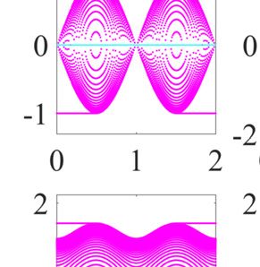
New J. Phys. 23 (2021) 073043                                                                  https://doi.org/10.1088/1367-2630/ac1287

                                 PAPER

                                 Real-potential-driven anti-PT -symmetry breaking in
O P E N AC C E S S
                                 non-Hermitian Su–Schrieffer–Heeger model
R E C E IVE D
12 April 2021
                                 Xuedong Zhao1 , Yan Xing1 , Lu Qi1 , Shutian Liu1 , ∗             , Shou Zhang2 and
                                 Hong-Fu Wang2 , ∗
R E VISE D
21 June 2021
                                 1
AC C E PTE D FOR PUBL IC ATION       School of Physics, Harbin Institute of Technology, Harbin, Heilongjiang 150001, People’s Republic of China
                                 2
8 July 2021                          Department of Physics, College of Science, Yanbian University, Yanji, Jilin 133002, People’s Republic of China
                                 ∗
                                     Authors to whom any correspondence should be addressed.
PUBL ISHE D
27 July 2021                     E-mail: stliu@hit.edu.cn and hfwang@ybu.edu.cn

                                 Keywords: anti-PT-symmetry breaking, topological phase, Su–Schrieffer–Heeger model
Original content from
this work may be used
under the terms of the
Creative Commons
Attribution 4.0 licence.         Abstract
Any further distribution         Non-Hermitian Hamiltonians with anti-PT symmetry show distinct discrepancies compared to
of this work must
maintain attribution to          PT -symmetric systems. Here we investigate the non-Hermitian Su–Schrieffer–Heeger (SSH)
the author(s) and the            model and reveal the interplay between anti-PT symmetry and different topological phases, in
title of the work, journal
citation and DOI.                which the anti-PT symmetry is triggered by introducing real chemical potential and imaginary
                                 nearest-neighbor hopping. Three types of anti-PT -symmetric SSH models with different on-site
                                 configurations are investigated, and the effect of each on-site configuration on the energy
                                 spectrum of system is analyzed and discussed. We find that the type of on-site configuration affects
                                 the energy spectrum of the same topological region significantly and each on-site configuration
                                 has distinguishable impacts on the energy spectra of different topological regions. Moreover, the
                                 spontaneous anti-PT -symmetry-breaking transitions undergone in both of the topologically
                                 trivial and nontrivial regions are also clarified. Furthermore, we address the corresponding
                                 eigenstates of some specific eigenvalues and some interesting localized phenomena are observed.
                                 Our results enrich the study of non-Hermitian topological phases and broaden the understanding
                                 of anti-PT -symmetric systems.

                                 1. Introduction

                                 Since the discovery of topological insulators, the topological states of matter have attracted extensive interest
                                 in photonics [1], condensed-matter physics [2, 3], and atomic and molecular physics [4]. As a Frontier,
                                 much attention has been paid to the exploration and investigation of these exotic materials [5–7] and many
                                 researchers have devoted their efforts to hunting for them. In general, topological insulators are insulated in
                                 bulk but support electrical conducting edges or surfaces and are characterized by nonvanishing bulk
                                 topological invariants [8–12]. In traditional topological band theory, topological insulators are classified by
                                 three discrete symmetries [13–16] and their dimensionality. The extraordinary features of topological
                                 insulators are the principle of the bulk-boundary correspondence [17–20] and the existence of robust
                                 ‘in-gap’ modes that are immune to local disorder and perturbations, including defects and thermal
                                 fluctuations. Specifically, as the simplest topological insulator, the one-dimensional Su–Schrieffer–Heeger
                                 (SSH) model [21] exhibits abundant physical phenomena, e.g. topological soliton excitation, fractional
                                 charge, and nontrivial gapless zero-energy edge state [22–28]. Furthermore, the topological properties of
                                 Bloch bands for the SSH model have been measured experimentally in a dimerized optical superconducting
                                 lattice [29].
                                     Contrary to the Hermitian operators in standard quantum mechanics [30], on the other hand, for open
                                 systems, it is commonly believed that the non-Hermitian operators possess complex eigenvalues and
                                 non-orthogonal eigenfunctions. However, in 1998, Bender and Boettcher [31] demonstrated that the
                                 non-Hermitian Hamiltonians with parity-time symmetry, where the parity-time symmetry corresponds to a
                                 combined symmetry of parity (P) symmetry and time-reversal (T ) symmetry, namely, [PT , H] = 0, can

                                 © 2021 The Author(s). Published by IOP Publishing Ltd on behalf of the Institute of Physics and Deutsche Physikalische Gesellschaft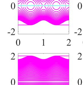
New J. Phys. 23 (2021) 073043                                                                        X Zhao et al

hold entirely real eigenvalues. More importantly, a spontaneous PT -symmetry-breaking transition will
occur once the parameter measuring non-Hermitian degree exceeds a definite threshold. The system in the
exact PT -symmetric phase not only can exhibit an entirely real energy spectrum but also shares common
eigenfunctions with the PT operator and all the eigenfunctions satisfy the PT symmetry, whereas the
eigenvalues of the Hamiltonian become partially or completely complex if the system is in
PT -symmetry-breaking phase and some or all of the eigenfunctions are neither the eigenfunctions of the
PT operator nor PT -symmetric. Motivated by this sensational discovery, various non-Hermitian
Hamiltonians with PT symmetry have been theoretically proposed in numerous literatures [32–38] and
different PT -symmetric systems have been experimentally realized based on diverse platforms [39–44].
Moreover, the topological phases of PT -symmetric systems have been analyzed and discussed intensively
[45–51] and numerous novel phenomena and applications in PT -symmetric topological systems have been
reported, such as robust edge state [52–55], high-order topological phase [56–61], topological energy
transfer [62], and so on.
    Inspired by the idea of PT symmetry, Ge et al proposed the concept of anti-PT -symmetric for the first
time [63], which implies that the commutator is replaced by the anticommutator or {PT , H} = 0. As an
extension of PT symmetry, the anti-PT -symmetric systems exhibit distinct discrepancies compared with
the PT -symmetric systems [64–66]. On a theoretical level, it turns out that the anti-PT -symmetric
systems can undergo a spontaneous anti-PT -symmetry-breaking transition, which is manifested by a
conversion from purely imaginary eigenvalue to complex or entirely real eigenvalues. From an experimental
perspective, the PT symmetry generally requires the introduction of balanced gain and loss to be
established, while one prominent advantage of the anti-PT -symmetric systems is that they can be
engineered and fabricated without any gain media, which is very attractive for the construction of
non-Hermitian quantum systems. Also, the anti-PT -symmetric systems have been realized in optical
systems [67–71], cold atoms [72], electrical circuits [73], and dissipatively coupled atomic beams [74]. Even
though the subject of topological insulators and the theories of both PT and anti-PT symmetries have
made significant progress in their respective domains, the investigation on the interplay between
anti-PT -symmetry and different topological phases is almost absent, thus it is meaningful to address and
reveal this interesting problem.
    In this paper, we consider three types of anti-PT -symmetric SSH models with different on-site
configurations and explore the interplay between anti-PT -symmetry and different topological phases. We
mainly focus on the effect of each on-site configuration with entirely real chemical potential on the energy
spectrum of system under the open boundary condition, and detailedly analyze and discuss the
spontaneous anti-PT -symmetry-breaking transitions that both of the topologically trivial and nontrivial
regions undergo. The results indicate that in both of the topologically trivial and nontrivial phases, the
systems exhibit novel and distinguishable behaviors. For the first on-site configuration in which a pair of the
positive and negative chemical potentials are located at the two ends of the lattice, we find that the anti-PT
symmetry in both of the topologically nontrivial regions is spontaneously broken for any nonvanishing
strength of the chemical potential γ, whereas the topologically trivial region undergoes an abrupt phase
transition from the exact anti-PT -symmetric phase to the mixed anti-PT -symmetric and broken phases at
a threshold and a second transition at another threshold. In the second on-site configuration, the positive
and negative chemical potentials are staggered. When γ is weak, the entirely real energy eigenvalues emerge
both in the two topologically nontrivial regions and at the two topological transition points. As γ continues
to increase, the entirely real energy eigenvalues also begin to emerge in the topologically trivial region. The
whole system exhibits an entirely real energy spectrum in the end and a transition from the mixed
anti-PT -symmetric and broken phases or the exact anti-PT -symmetric phase to the fully anti-PT -broken
phase occurs. The third on-site configuration is that the positive and negative chemical potentials are
separately distributed on the half of the lattice. Compared with the two preceding configurations, one can
observe that the topologically nontrivial regions show some unique properties. For weak γ, there are a pair
of conjugated purely imaginary and two entirely real energy eigenvalues in both of the topologically
nontrivial regions, and the rest of the energy eigenvalues are complex. With the increase of γ, the pair of
conjugated purely imaginary energy eigenvalues gradually become entirely real, i.e. the topologically
nontrivial regions undergo a phase transition from the mixed anti-PT -symmetric and broken phases to the
fully anti-PT -broken phase. However, the anti-PT symmetry in the topologically trivial region is fully
broken all the time. We also address the populations of some special eigenstates therein and capture some
interesting localized phenomena.
    The remainder of this paper is organized as follows. In section 2, the Hamiltonians of the three types of
anti-PT -symmetric SSH models with different on-site configurations are presented. In section 3, the effect
of each on-site configuration with entirely real chemical potential on the energy spectrum of system and the
spontaneous anti-PT -symmetry-breaking transition in both the topologically trivial and nontrivial regions

                                             2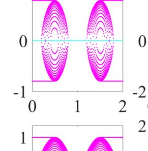
New J. Phys. 23 (2021) 073043                                                                                                   X Zhao et al

   Figure 1. Schematic diagrams of the non-Hermitian SSH models with three different on-site configurations. The orange and
   blue solid circles denote the two sublattices and the brown (black) double arrow represents the forward and backward purely
   imaginary tunneling amplitudes of intracell (intercell). The on-site configurations are respectively governed by Ho1 , Ho2 , and Ho3
   from top to bottom. All the three types of non-Hermitian SSH models satisfy the anti-PT symmetry.

are analyzed and discussed detailedly. Moreover, the populations of some special eigenstates are also
displayed. Finally, a conclusion is given in section 4.

2. Model and Hamiltonian

We consider a non-Hermitian counterpart of the SSH model composed of even N sites, which is
characterized by the purely imaginary dimerized nearest-neighbor hopping, as described by the following
Hamiltonian [75]
                            f †                            f †
                    Hh =        T1 cn+1 cn + T1b cn† cn+1 +    T2 cn+1 cn + T2b cn† cn+1 .             (1)
                                 n∈odd                                    n∈even

    Here cn† (cn ) is the creation (annihilation) operator of particle at site n, Ti and Tib are the forward and
                                                                                                  f

                                                                                             f
backward tunneling amplitudes of intracell (i = 1) or intercell (i = 2), respectively, T1 = T1b = iJ1 ,
  f
T2 = T2b = iJ2 with J1 = J − λ cos (Φ) and J2 = J + λ cos (Φ) are the hopping coefficients of the
conventional SSH model, where λ is the strength of dimerization and Φ ∈ [0, 2π] is the periodic parameter.
Such a model can be mapped to the binary optical waveguide array intimately and the purely imaginary
coupling can be realized by incorporating assistant optical waveguides into the bare array and further
resorting to adiabatic elimination [64, 76].
                                            For   convenience, we set J = 1 as the energy unit hereafter. The
                                       f         ∗
system will become Hermitian if Ti = Tib . Here, we consider three types of on-site configurations with
entirely real chemical potential, which are respectively governed as follows

                                      Ho1 = γ c1† c1 − cN† cN ,


                                      Ho2 = γ          cn† cn −          cn† cn ,
                                                 n∈odd             n∈even                                        (2)
                                               ⎛                                         ⎞

                                      Ho3 = γ ⎝             cn† cn −              cn† cn ⎠ ,
                                                 n∈[1, N2 ]          n∈[ N2 +1,N ]

where Ho1 denotes that only the two ends of the lattice have the entirely real chemical potential γ (the 1st
site) and −γ (the Nth site), Ho2 represents that the entirely real chemical potential γ is located at odd site,
whereas −γ is located at even site, and Ho3 shows that each site has the entirely real chemical potential,
indicating that the entirely real chemical potential γ is located at one half of the lattice and −γ is located at
the other half of the lattice. Therefore, the Hamiltonian of the whole system can be written as below

                                                   H = Hh + Hoi         (i = 1, 2, 3),                                                   (3)

and the schematic diagrams of the three models are respectively sketched in figure 1. Furthermore, all the
Hamiltonians of the three models meet a combined anti-symmetry of P symmetry and T symmetry, where
                                                            †
the operations of P and T operators satisfy Pcn† (cn ) P = cN−n +1 (cN−n+1 ) and T iT = −i, respectively. It is
evident that all the three Hamiltonians satisfy the anti-PT symmetry {PT , H} = 0, namely,
PT H(PT )−1 = PT HT P = −H. Compared with the energy eigenvalues of the PT -symmetric system
emerging in conjugate pairs, the anti-PT -symmetry ensures the energy eigenvalues in pairs with identical
imaginary part and opposite real part.

                                                        3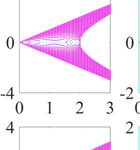
New J. Phys. 23 (2021) 073043 X Zhao et al
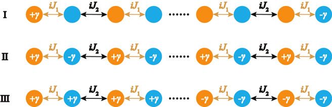
Figure 2. (a) The real and imaginary parts of energy spectrum of the anti-PT -symmetric SSH model with the strength of the
chemical potential γ = 0 as a function of Φ. Here N = 100, λ = 0.5, and the red points label the twofold degenerate zero-energy
edge states. (b) Zak phase Θ1 as a function of Φ.
In the following we explore the novel and unique properties of all the three types of anti-PT -symmetric
SSH models from the perspective of the energy spectrum, respectively, and further reveal the interplay
between anti-PT symmetry and different topological phases.
3. Analyses and discussions
In this section, the energy spectrum of the anti-PT -symmetric SSH model under the open boundary
condition is exhibited to study the interplay between anti-PT symmetry and different topological phases,
and the effects of the three types of on-site configurations on the real and imaginary parts of the energy
spectrum in different topological phase regions are analyzed and discussed, respectively. Furthermore, we
also depict some special eigenstates therein and the analytical results of the edge states in each case are
detailed in appendix.
Without loss of generality, we start with the on-site configuration in the absence of entirely real chemical
potential. In this case the non-Hermitian SSH model is not only anti-PT -symmetric, but also
anti-Hermitian, satisfying H = −H† . As detailed in references [77, 78], the anti-Hermitian topological
insulators can merely hold purely imaginary energy eigenvalues and the corresponding eigenstates are all
orthogonal to each other. Moreover, they can share the same topological transition points with their
Hermitian counterparts. To this end, we plot the real and imaginary parts of the energy spectrum as a
function of Φ, as shown in figure 2(a). One can observe that when the strength of the chemical potential
γ = 0, the system exhibits a purely imaginary energy spectrum and the imaginary part of the energy
spectrum essentially has the identical band structure with the conventional SSH model, which indicates that
the anti-PT symmetry of the whole system is preserved. Specifically, when 0 Φ < π2 and 3π 2 < Φ 2π,
the system is in the topologically nontrivial phase and characterized by the emergence of the twofold
degenerate zero-energy edge states that are localized either on the left or on the right boundary of the
system, which means that only the two edge states are dynamically stable. On the contrary, the twofold
degenerate zero-energy edge states are not supported within the bulk gap in the region of π2 < Φ < 3π 2
and
the system is thus topologically trivial and dynamically unstable. It is visible that the bulk gap closes and
reopens at the topological transition points Φ = π2 and 3π 2
in conformity to the conventional SSH model.
In order to further demonstrate the topological property of the anti-PT -symmetric SSH model, by
employing Fourier transformation cα,j = √1M k eikj cα,k with M being the total number of unit cells and α
taking the sublattices A or B, the Hamiltonian of the system in momentum space can be written in the form
of
Hh (k) = ψk† h(k)ψk , (4)
4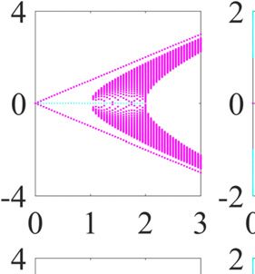
New J. Phys. 23 (2021) 073043                                                                        X Zhao et al

                     T
where ψk = cA,k , cB,k and

                                                   0          iJ1 + iJ2 e−ik
                                    h(k) =                                     .                             (5)
                                              iJ1 + iJ2 eik         0
Diagonalizing equation (5), we can get two bands

                                    E(k) = ±i J12 + J22 + 2J1 J2 cos k.                                      (6)

Both the bands are purely imaginary but the imaginary parts are consistent with the energy eigenvalues of
the conventional SSH model in momentum space, viz, there is a gap between these bands as long as J1 = J2
and they touch once J1 = J2 . When the two purely imaginary bands are separated, each band is relevant to a
Zak phase defined as
                                          Θn = i      dk Ln | ∂k |Rn  ,                                    (7)

where n = 1 (2) labels the upper (lower) purely imaginary band, |Rn  and |Ln  are the right and left
eigenstates from h(k) and h† (k), respectively. We calculate the Zak phase for each band when Φ = π2 and 3π 2
(J1 = J2 ) and Θ1 as a function of Φ is shown in figure 2(b). One can observe that Θ1 = π if 0  Φ < π2 and
3π
 2
    < Φ  2π (J1 < J2 ) and Θ1 = 0 if π2 < Φ < 3π  2
                                                     (J1 > J2 ). While a vanishing Θ1 indicates a topologically
trivial phase, a nonzero Θ1 characterizes a topologically nontrivial one and a pair of zero-energy edge states
emerge in the energy spectrum of the system. Furthermore, the profile of Θ2 is identical to Θ1 .

3.1. The first on-site configuration
We first consider the on-site configuration that a pair of the positive and negative chemical potentials are
located at the two ends of the lattice, respectively. The Hamiltonian of the system under this circumstance is
governed by
                                                  H = Hh + Ho1 .                                           (8)
Figures 3 and 4 exhibit the numerically calculated energy spectra for different system parameters. The real
and imaginary parts of the energy spectrum as a function of Φ are displayed in figure 3. We first focus on
the topologically nontrivial regions 0  Φ < π2 and 3π     2 < Φ  2π. For the case of γ being weak, such as
γ = 0.1, two entirely real energy eigenvalues with the form of ±a (a > 0) emerge in both of the topological
nontrivial regions, as shown in figure 3(a). Actually, we find that the energy spectra in both of the
topologically nontrivial regions are always comprised of two entirely real energy eigenvalues and N − 2
conjugated purely imaginary energy eigenvalues as long as γ is nonzero, which means that the system is in
the mixed anti-PT -symmetric and broken phases all the time, as shown in figures 3(b)–(e).
    On the other hand, the topologically trivial region π2 < Φ < 3π   2
                                                                        shows more abundant features with the
increase of γ, which is obviously different from the topologically nontrivial regions. To be concrete, for
weak γ, the system is capable of possessing a purely imaginary energy spectrum, as shown in figure 3(a),
which implies that the anti-PT symmetry of this region is unbroken. As γ increases, the purely imaginary
energy spectrum can be maintained until γ exceeds a threshold γ c1 (Φ) and four conjugated complex energy
eigenvalues with the form of ±a ± ib (a, b > 0) will emerge, which indicates a transition from the exact
anti-PT -symmetric phase to the mixed anti-PT -symmetric and broken phases. The transition initially
occurs at Φ = π with γ c1 (π) = 0.506 and eventually terminates at the two topological transition points
with γc1 ( π2 ) = γc1 ( 3π
                         2 ) = 1. Definitely, the system has unbroken anti-PT -symmetric phase in this region
when 0.506 < γ < 1 and the whole system covering both the topologically trivial and nontrivial regions is
in the mixed anti-PT -symmetric and broken phases when γ = 1, as shown in figures 3(b) and (c).
Interestingly, a novel phenomenon arises in this region when γ > 1. We find another transition manifested
by the bifurcation of the real parts of the four conjugated complex energy eigenvalues until γ is beyond a
second threshold γ c2 (Φ), corresponding to the two pairs of conjugated complex energy eigenvalues
converting into four entirely real energy eigenvalues with the form of ±a1 and ±a2 (a1 , a2 > 0), as shown in
figure 3(d). The second transition extends from the two topological transition points to Φ = π with
increasing γ and the energy spectrum in the whole topologically trivial region is composed of four entirely
real energy eigenvalues and N − 4 conjugated purely imaginary energy eigenvalues when
γ > γ c2 (π) = 2.914, as shown in figure 3(e). Moreover, the whole system is in the mixed
anti-PT -symmetric and broken phases.
    In order to address the interplay between anti-PT symmetry and different topological phases more
profoundly, figure 4 exhibits the real and imaginary parts of the energy spectrum in different topological
phase regions versus γ. The situations for the topologically nontrivial phase with Φ = 0, topological
transition points with Φ = π2 , and topologically trivial phase with Φ = π are shown in figures 4(a)–(c),
respectively. What one can see is that two entirely real energy eigenvalues emerge in the topologically

                                             5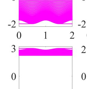
New J. Phys. 23 (2021) 073043                                                                                             X Zhao et al

   Figure 3. The real and imaginary parts of energy spectrum of the anti-PT -symmetric SSH model with the first on-site
   configuration as a function of Φ. The strength of the chemical potential γ = (a) 0.1, (b) 0.8, (c) 1.2, (d) 2.2, and (e) 3.1,
   respectively. Here N = 100, λ = 0.5, and the magenta points label the entirely real and conjugated complex energy eigenvalues.

nontrivial regions once γ = 0 and their absolute values will increase with the increase of γ. Moreover, two
pairs of conjugated complex energy eigenvalues in the topologically trivial region will emerge at a threshold
γ c1 before which the system exhibits a purely imaginary energy spectrum and is thus in the exact
anti-PT -symmetric phase. As γ increases unceasingly, the real parts of the two pairs of conjugated complex
energy eigenvalues split into four parts and their imaginary parts shrink into zero at a second threshold γ c2
after which a pair of entirely real energy eigenvalues tends to zero in the limit of γ → ∞. Additionally, when
Φ approaches to the two topological transition points, γ c1 increases but γ c2 decreases, which reflects that the
initial occurrence of the first transition is at Φ = π, whereas the second transition ultimately ends at it
indeed, and γ c1 and γ c2 will merge at the two topological transition points.
     Furthermore, the populations of some special eigenstates belonging to different topological phase
regions are displayed in figure 5. Figure 5(a) depicts the populations of eigenstates with the two entirely real
energy eigenvalues ±a emerging in the topologically nontrivial regions when Φ = 0 and γ = 4, which are

                                                      6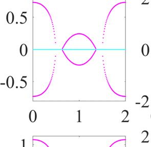
New J. Phys. 23 (2021) 073043                                                                                            X Zhao et al

   Figure 4. The real and imaginary parts of energy spectra in different topological phase regions versus γ for the
   anti-PT -symmetric SSH model with the first on-site configuration. Here Φ = (a) 0, (b) π2 , and (c) π, respectively. The magenta
   points label the entirely real and conjugated complex energy eigenvalues.

symmetrically localized on the left and right boundaries of the system. Figure 5(b) shows the eigenstates of
the two pairs of conjugated complex energy eigenvalues emerging in the topologically trivial region with
Φ = π and γ = 2 and the energy eigenvalues a ± ib correspond to the left-edge-localized states with an
identical population, the eigenstates for the energy eigenvalues −a ± ib are the right-edge-localized states
with an identical population. Also, the eigenstates of the four entirely real energy eigenvalues ±a1 and ±a2
(a1 > a2 ) emerging in the topologically trivial region with Φ = π and γ = 4 are depicted in figures 5(c) and
(d), respectively, all of which describe two pairs of symmetrically edge-localized states.
    The preceding analyses and discussions elucidate that although the effects of the first on-site
configuration on the topologically trivial and nontrivial regions are considerably different, the whole system
is at most in the mixed anti-PT -symmetric and broken phases no matter how large γ is.

3.2. The second on-site configuration
We next consider the on-site configuration that the positive and negative chemical potentials are staggered
and the Hamiltonian of the system now reads

                                                          H = Hh + Ho2 .                                                            (9)

In figure 6, we show the real and imaginary parts of the energy spectrum as a function of Φ. When γ is
weak, as shown in figure 6(a), both the topologically nontrivial regions and topological transition points
contain two entirely real energy eigenvalues with the form of ±a (a > 0), the topologically trivial region
exhibits a purely imaginary energy spectrum nonetheless, which is different from the first configuration. As
γ increases, the number of the entirely real energy eigenvalues at the two topological transition points
begins to increase and the behavior will extend to both the topologically trivial and nontrivial regions,
meanwhile, the number of the purely imaginary energy eigenvalues reduces accordingly and the gaps in the
imaginary part of the energy spectrum gradually shrink to vanish, as shown in figures 6(b)–(d). As γ
continues to increase until γ  2, the whole system can exhibit an entirely real energy spectrum, as shown
in figures 6(e) and (f).

                                                      7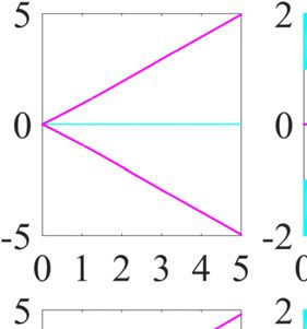
New J. Phys. 23 (2021) 073043                                                                                             X Zhao et al

   Figure 5. The populations of eigenstates for (a) the two entirely real energy eigenvalues ±a in the topologically nontrivial
   regions with Φ = 0 and γ = 4, (b) the two pairs of conjugated complex energy eigenvalues a ± ib (left) and −a ± ib (right) in
   the topologically trivial region with Φ = π and γ = 2, and the four entirely real energy eigenvalues (c) ±a1 and (d) ±a2
   (a1 > a2 ) in the topologically trivial region with Φ = π and γ = 4.

    We also plot the real and imaginary parts of the energy spectrum in different topological phase regions
versus γ by respectively choosing Φ = 0, π2 , and π, as shown in figure 7. Figure 7(a) indicates that two
entirely real energy eigenvalues emerge in the topologically nontrivial regions for weak γ and their
corresponding eigenstates with γ = 1 are depicted in figure 8, which also captures the states symmetrically
localized on the left and right boundaries of the system. It is clear that with the increase of γ, more and
more purely imaginary energy eigenvalues convert into entirely real energy eigenvalues, thus the moduli of
the purely imaginary energy eigenvalues decrease, whereas the absolute values of the entirely real energy
eigenvalues increase. Furthermore, the energy spectrum of the system at the topological transition points
are immediately accompanied by the emergence of large-scale entirely real energy eigenvalues, as shown in
figure 7(b). Subsequently, the behavior occurs in both the topologically trivial and nontrivial regions, as
shown in figures 7(a) and (c). All the purely imaginary energy eigenvalues become entirely real when γ  2
and there is only an entirely real energy spectrum left.
    The second on-site configuration has a similar effect for both of the topologically trivial and nontrivial
regions and can induce a transition from the mixed anti-PT -symmetric and broken phases to the fully
anti-PT -broken phase. Consequently, the system holds two different phases in the topologically nontrivial
regions, i.e. the mixed anti-PT -symmetric and broken phases and the fully anti-PT -broken phase, while
the system can undergo a transition from the exact anti-PT -symmetric phase to the mixed
anti-PT -symmetric and broken phases further to the fully anti-PT -broken phase in the topologically
trivial region. In brief, the whole system can be in the fully anti-PT -broken phase with the increase of γ.

                                                      8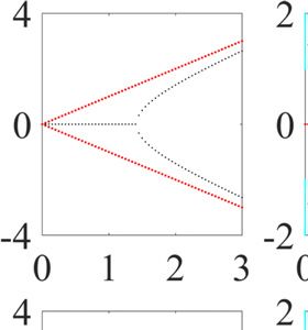
New J. Phys. 23 (2021) 073043                                                                                                   X Zhao et al

   Figure 6. The real and imaginary parts of energy spectrum of the anti-PT -symmetric SSH model with the second on-site
   configuration as a function of Φ. The strength of the chemical potential γ = (a) 0.05, (b) 0.8, (c) 1, (d) 1.5, (e) 2, and (f) 3,
   respectively. Here N = 100, λ = 0.5, and the magenta points label the entirely real energy eigenvalues.

3.3. The third on-site configuration
We now turn to the on-site configuration that the positive and negative chemical potentials are separately
distributed on the half of the lattice, the Hamiltonian of the system in this case can be written as

                                                             H = Hh + Ho3 .                                                           (10)

                                                         9
New J. Phys. 23 (2021) 073043 X Zhao et al
Figure 7. The real and imaginary parts of the energy spectra in different topological phase regions versus γ for the
anti-PT -symmetric SSH model with the second on-site configuration. Here Φ = (a) 0, (b) π2 , and (c) π, respectively. The
magenta points label the entirely real energy eigenvalues.
Figure 8. The populations of the eigenstates for the two entirely real energy eigenvalues ±a in the topologically nontrivial
regions with Φ = 0 and γ = 1.
Analogous to the first two configurations, as γ increases, we present the real and imaginary parts of the
energy spectrum as a function of Φ in figure 9. It now turns out that the energy spectrum in the
topologically trivial region consists of N2 pairs of conjugated complex energy eigenvalues all the time no
matter how large γ is and the absolute values of the real parts of these conjugated complex energy
eigenvalues become almost equal with the increase of γ, whereas their imaginary parts are immune to the
increase of γ and remain unchanged, as shown in figures 9(a)–(e). By contrast, there are some unique
properties in both of the topologically nontrivial regions. Concretely, when γ is weak, apart from the N − 4
conjugated complex energy eigenvalues, two entirely real energy eigenvalues with the form of ±a1 (a1 > 0)
and two purely imaginary energy eigenvalues with the form of ±ib (b > 0) also emerge in both of the
regions, as shown in figure 9(a). As γ increases up to γ = 0.251, an interesting phenomenon that the pair of
conjugated purely imaginary energy eigenvalues converting into two entirely real energy eigenvalues with
the form of ±a2 (a2 > 0) arises. The behavior initially occurs in the vicinity of the two topological
transition points and eventually terminates at Φ = 0 and 2π with further increasing γ, as shown in
10New J. Phys. 23 (2021) 073043 X Zhao et al
Figure 9. The real and imaginary parts of energy spectrum of the anti-PT -symmetric SSH model with the third on-site
configuration as a function of Φ. The strength of the chemical potential γ = (a) 0.2, (b) 0.8, (c) 1.415, (d) 4, and (e) 8,
respectively. Here N = 100 and λ = 0.5. The red points label the entirely real energy eigenvalues and the black points label the
purely imaginary energy eigenvalues which will become entirely real with the increase of γ.
figure 9(b). When γ = 1.415, the two purely imaginary energy eigenvalues in both of the regions
completely become entirely real, as shown in figure 9(c). As γ increases continuously, the absolute values of
the two newly emerging entirely real energy eigenvalues increase and the real part of the whole energy
spectrum in Φ ∈ [0, 2π] becomes narrower, as shown in figures 9(d)–(e).
In figure 10, we plot the real and imaginary parts of the energy spectrum of different topological phase
regions for Φ = 0, π2 , and π versus γ. It is visible that there are always two entirely real energy eigenvalues
and two purely imaginary energy eigenvalues in the topologically nontrivial regions when γ is moderate. As
γ increases, when the moduli of the two purely imaginary energy eigenvalues decrease, the absolute values
of the real parts of the rest of energy eigenvalues including the two entirely real energy eigenvalues increase
and become almost equal. As further increasing γ, the two purely imaginary energy eigenvalues coalesce at
zero energy followed by the emergence of two extra entirely real energy eigenvalues, as shown in
11New J. Phys. 23 (2021) 073043 X Zhao et al
Figure 10. The real and imaginary parts of energy spectra in different topological phase regions versus γ for the
anti-PT -symmetric SSH model with the third on-site configuration. We choose Φ = (a) 0, (b) π2 , and (c) π, respectively. The
red points label the entirely real energy eigenvalues and the black points label the purely imaginary energy eigenvalues which will
become entirely real with the increase of γ.
figure 10(a). Similarly, the absolute values of the real parts of these N2 pairs of conjugated complex energy
eigenvalues in the topologically trivial region and at the topological transition points also increase and the
difference among them decreases with the increase of γ, as shown in figures 10(b) and (c).
Furthermore, figures 11(a)–(c) display the populations of some special eigenstates belonging to the
topologically nontrivial regions with Φ = 0. The populations of eigenstates corresponding to two entirely
real energy eigenvalues ±a1 with γ = 4 are depicted in figure 11(a), which describe the states symmetrically
localized on the left and right boundaries of the system. Nevertheless, the eigenstates of both the two purely
imaginary energy eigenvalues ±ib and two newly emerging entirely real energy eigenvalues ±a2 correspond
to the bound states mainly concentrated in the center of the lattice, as respectively depicted in figures 11(b)
and (c) with γ = 0.8 and 2. It is worth mentioning that a unique distribution is manifested by the
eigenstates of these conjugated complex energy eigenvalues in the whole region Φ ∈ [0, 2π] of the energy
spectrum. In other words, when all the corresponding eigenstates are extended, they show the semi-lattice
localization behavior depending on the sign of the real parts of these conjugated complex energy
eigenvalues solely. When the real parts are positive (negative), the corresponding eigenstates are only
localized on the left- (right-) half part of the lattice. In figure 11(d), we show the situation of Φ = π2 and
γ = 0.8 for the energy eigenvalues 0.8 + 1.996i (left) and −0.8 + 1.996i (right).
Overall, as γ increases, the third on-site configuration mainly affects the topologically nontrivial regions
where the conversion of the purely imaginary energy eigenvalues into the entirely real energy eigenvalues for
the two bound states leads to a transition from the mixed anti-PT -symmetric and broken phases to the
fully anti-PT -broken phase, whereas the topologically trivial region is in the fully anti-PT -broken phase
from the outset.
12New J. Phys. 23 (2021) 073043 X Zhao et al
Figure 11. The populations of the eigenstates belonging to the topologically nontrivial region Φ = 0 for (a) the two entirely real
energy eigenvalues ±a1 with γ = 4, (b) the two purely imaginary energy eigenvalues ±ib with γ = 0.8, and (c) the two newly
emerging entirely real energy eigenvalues ±a2 with γ = 2. (d) Semi-lattice localized eigenstates for the two sample conjugated
complex energy eigenvalues 0.8 + 1.996i (left) and −0.8 + 1.996i (right) with Φ = π2 and γ = 0.8.
4. Conclusions
In conclusion, we have considered three types of anti-PT -symmetric SSH models and explored the
interplay between anti-PT symmetry and different topological phases. We detailedly analyze and discuss
the effect of different on-site configurations on the energy spectrum of the system. Specifically, in the first
on-site configuration, with the increase of the strength of chemical potential, the energy spectra in both of
the topologically nontrivial regions always consist of two entirely real and N − 2 purely imaginary energy
eigenvalues. While the system initially exhibits a purely imaginary energy spectrum in the topologically
trivial region. When the strength of chemical potential continues to increase, two pairs of conjugated
complex energy eigenvalues emerge and further convert into four entirely real energy eigenvalues.
Ultimately, there are four entirely real and N − 4 purely imaginary energy eigenvalues in the energy
spectrum in the topologically trivial region. As a result, the system in the topologically nontrivial regions is
in the mixed anti-PT -symmetric and broken phases all the time but the system in the topologically trivial
region undergoes a transition from the exact anti-PT -symmetric phase to the mixed anti-PT -symmetric
and broken phases. In the second on-site configuration, when the strength of chemical potential is weak, the
energy spectra in both of the topologically nontrivial regions and the topological transition points contain
two entirely real energy eigenvalues, whereas the energy spectrum in the topologically trivial region remains
purely imaginary. As the strength of chemical potential increases ceaselessly, the energy spectrum of the
whole system undergoes a process characterized by large-scale purely imaginary energy eigenvalues
converting into entirely real energy eigenvalues. In the end, there is only an entirely real energy spectrum
left, which implies that the topologically nontrivial and trivial regions of the system undergo a transition
13New J. Phys. 23 (2021) 073043 X Zhao et al
from the mixed anti-PT -symmetric and broken phases to the fully anti-PT -broken phase and from the
exact anti-PT -symmetric phase to the fully anti-PT -broken phase, respectively. In the third on-site
configuration, the energy spectrum in the topologically trivial region is consisted of N2 pairs of conjugated
complex energy eigenvalues and there are N2 − 2 pairs of conjugated complex and two entirely real energy
eigenvalues in both of the topologically nontrivial regions as long as the strength of chemical potential is
nonvanishing. Moreover, a pair of conjugated purely imaginary energy eigenvalues can also be found in
both of the topologically nontrivial regions, which will convert into two entirely real energy eigenvalues
once the strength of chemical potential exceeds a threshold. These aforesaid results indicate that the system
in the topologically trivial region is in the fully anti-PT -broken phase from the outset, and both of the
topologically nontrivial regions of the system undergo a transition from the mixed anti-PT -symmetric and
broken phases to the fully anti-PT -broken phase. Furthermore, the populations of some special eigenstates
in each case are also addressed and a few interesting localized phenomena are observed. Our work would
further deepen the understanding of the interplay between anti-PT symmetry and different topological
phases and provide helpful insights for the study of non-Hermitian topological systems.
Acknowledgments
This work was supported by the National Natural Science Foundation of China under Grant Nos. 61822114,
12074330, 11874132, 62071412, and 61575055.
Data availability statement
All data that support the findings of this study are included within the article (and any supplementary files).
Appendix A. Solutions of the edge states
In this appendix, for all the three cases in the main text, we solve the left and right edge states emerging in
both the topological nontrivial regions analytically.
For the sake of clarity, we rewrite the Hamiltonian of the first case as follows
†
Hh = iJ1 aj bj + iJ2 b†j aj+1 + iJ1 b†j aj + iJ2 a†j+1 bj ,
j
(A.1)
Ho1 =γ a†1 a1 − b†M bM ,
where aj (bj ) and a†j (b†j ) are the annihilation and creation operators of particle at site A (B) in the jth unit
cell, respectively. Even M is the total number of unit cells. J1 and J2 have the same definition as the main
text. The Hamiltonian of the whole system reads
H = Hh + Ho1 . (A.2)
We resort to the transfer matrix method to calculate the edge states. For a single-particle eigenstate
† †
Ψ= M j=1 Φj,A aj |0 + Φj,B bj |0 with an energy eigenvalue E, where Φj,A and Φj,B are the wave functions at
sites A and B in the jth unit cell, respectively, the Schrödinger equation can be derived as
(E − γ) Φ1,A = iJ1 Φ1,B ,
EΦj,A = iJ1 Φj,B + iJ2 Φj−1,B , j ∈ (1, M] ,
(A.3)
EΦj,B = iJ1 Φj,A + iJ2 Φj+1,A , j ∈ [1, M) ,
(E + γ) ΦM,B = iJ1 ΦM,A .
14New J. Phys. 23 (2021) 073043 X Zhao et al
Sublattice A in equation (A.3) can be eliminated and we obtain
2
E + γE + J12 ΦM,B = −J1 J2 ΦM−1,B ,
2
E + J12 + J22 Φj,B = −J1 J2 Φj−1,B + Φj+1,B , j ∈ (1, M) ,
(A.4)
E 2
E2 + J1 + J22 Φ1,B = −J1 J2 Φ2,B .
E−γ
Similarly, we can also eliminate sublattice B in equation (A.3) and obtain
2
E − γE + J12 Φ1,A = −J1 J2 Φ2,A ,
2
E + J12 + J22 Φj,A = −J1 J2 Φj−1,A + Φj+1,A , j ∈ (1, M) ,
(A.5)
E 2
E2 + J1 + J22 ΦM,A = −J1 J2 ΦM−1,A .
E+γ
By employing transfer matrix method, equations (A.4) and (A.5) can be rewritten as follows
T T
Φ2,A Φ1,A = T1 Φ1,A Φ0,A ,
T T
Φj+1,A Φj,A = T Φj,A Φj−1,A , j ∈ (1, M) ,
T T
ΦM−1,A ΦM,A = T2 ΦM,A ΦM +1,A ,
T T (A.6)
Φ2,B Φ1,B = T3 Φ1,B Φ0,B ,
T T
Φj−1,B Φj,B = T Φj,B Φj+1,B , j ∈ (1, M) ,
T T
ΦM−1,B ΦM,B = T4 ΦM,B ΦM +1,B ,
here, these transfer matrices take the form
ν −1 μ1 0
T= , T1 = ,
1 0 1 0
ϕ1 0 ϕ2 0
T2 = , T3 = , (A.7)
1 0 1 0
μ2 0
T4 = ,
1 0
E J 2 +J 2
E2 + E+
E2 +J12 +J22 ) E2 −γE+J12 ) E2 +γE+J12 )
where ν = − ( J1 J2
, μ1 = − ( J1 J2
, μ2 = − ( J1 J2
, ϕ1 = − γ 1
J1 J2
2
, and
2 E 2
E + E−γ J1 +J2 2
ϕ2 = − J1 J2
.
We can diagonalize the transfer matrix T, that is, D = U−1 TU,
β− 0 β− β+
D= , U= ,
0 β+ 1 1
(A.8)
1 −1 β+
U −1 = √ 2 ,
ν −4 1 −β−
√
ν±ν −4 2
where β± = 2
.
Therefore, under the open boundary condition, Φ0,A = Φ0,B = ΦM+1,A = ΦM+1,B = 0, an arbitrary
single-particle eigenstate Ψ satisfies
j−1 j−1
Φj+1,A 1 β + β − − μ1 β −
= √ 2 U j−1 j−1 Φ1,A ,
Φj,A ν −4 μ1 β + − β − β +
j−1 j−1
Φj+1,B 1 β+ β− − ϕ2 β− E−γ (A.9)
= √ 2 U j−1 j−1 Φ1,A .
Φj,B ν −4 ϕ2 β+ − β− β+ iJ1
15New J. Phys. 23 (2021) 073043 X Zhao et al
According to equation (A.9), in the large M limit, we can conclude that the necessary conditions for the
existence of the edge state localized on the left boundary are β + = μ1 = ϕ2 and |β− | > 1. The energy
eigenvalue of the left edge state is governed by
2
J22 J2
γ− γ + γ − γ2 + 4 J22 − J12
EL = . (A.10)
2
Also, the solution for the energy eigenvalue of the right edge state is
J22 J2 2
γ− γ + γ − γ2 + 4 J22 − J12
ER = − . (A.11)
2
For the second case, the Hamiltonian of the on-site configuration is described by
†
Ho2 = γ aj aj − b†j bj . (A.12)
j
We can write the Schrödinger equation as follows
(E − γ) Φ1,A = iJ1 Φ1,B ,
(E − γ) Φj,A = iJ1 Φj,B + iJ2 Φj−1,B , j ∈ (1, M] ,
(A.13)
(E + γ) Φj,B = iJ1 Φj,A + iJ2 Φj+1,A , j ∈ [1, M) ,
(E + γ) ΦM,B = iJ1 ΦM,A .
The energy eigenvalues of the left and right edge states in the large M limit are EL = +γ and ER = −γ,
respectively. For the edge state localized on the left boundary, the wave functions are Φj,B = 0 and
j−1 M−j
Φj,A = − JJ12 Φ1,A , the wave functions of the right edge state satisfy Φj,A = 0 and Φj,B = − JJ21 ΦM,B .
The Hamiltonian of the third on-site configuration reads
†
Ho3 = γ aj aj + b†j bj − γ a†j aj + b†j bj . (A.14)
j∈[1, M
2 ] j∈[ M +1,M
2 ]
The Schrödinger equation is given by
(E − γ) Φ1,A = iJ1 Φ1,B ,
M
(E − γ) Φj,A = iJ1 Φj,B + iJ2 Φj−1,B , j∈ 1, ,
2
M
(E + γ) Φj,A = iJ1 Φj,B + iJ2 Φj−1,B , j∈ + 1, M ,
2
(A.15)
M
(E − γ) Φj,B = iJ1 Φj,A + iJ2 Φj+1,A , j ∈ 1, ,
2
M
(E + γ) Φj,B = iJ1 Φj,A + iJ2 Φj+1,A , j∈ + 1, M ,
2
(E + γ) ΦM,B = iJ1 ΦM,A .
When M is large enough, the energy eigenvalues of the left and right edge states are EL = +γ and
j−1
ER = −γ, respectively. The wave functions of the left edge state are Φj,B = 0, Φj,A = − JJ21 Φ1,A with
M M
j ∈ 1, 2 , and Φj,A = 0 with j ∈ 2 + 1, M . For the right edge state, the wave functions are Φj,A = 0,
M−j
Φj,B = − JJ21 ΦM,B with j ∈ M2 + 1, M , and Φj,B = 0 with j ∈ 1, M2 .
ORCID iDs
Shutian Liu https://orcid.org/0000-0001-9748-0175
Hong-Fu Wang https://orcid.org/0000-0002-6778-6330
16New J. Phys. 23 (2021) 073043 X Zhao et al
References
[1] Ozawa T et al 2019 Rev. Mod. Phys. 91 015006
[2] Hasan M Z and Kane C L 2010 Rev. Mod. Phys. 82 3045
[3] Qi X-L and Zhang S-C 2011 Rev. Mod. Phys. 83 1057
[4] Dalibard J, Gerbier F, Juzeliūnas G and Öhberg P 2011 Rev. Mod. Phys. 83 1523
[5] Lee D-H, Zhang G-M and Xiang T 2007 Phys. Rev. Lett. 99 196805
[6] Fu L and Kane C L 2008 Phys. Rev. Lett. 100 096407
[7] Agapito L A, Kioussis N, Goddard W A and Ong N P 2013 Phys. Rev. Lett. 110 176401
[8] Niu Q, Thouless D J and Wu Y-S 1985 Phys. Rev. B 31 3372
[9] Aoki H and Ando T 1986 Phys. Rev. Lett. 57 3093
[10] Yu R, Qi X L, Bernevig A, Fang Z and Dai X 2011 Phys. Rev. B 84 075119
[11] Leykam D, Bliokh K Y, Huang C, Chong Y D and Nori F 2017 Phys. Rev. Lett. 118 040401
[12] Shen H, Zhen B and Fu L 2018 Phys. Rev. Lett. 120 146402
[13] Schnyder A P, Ryu S, Furusaki A and Ludwig A W W 2008 Phys. Rev. B 78 195125
[14] Ryu S, Schnyder A P, Furusaki A and Ludwig A W W 2010 New J. Phys. 12 065010
[15] Chiu C K, Teo J C Y, Schnyder A P and Ryu S 2016 Rev. Mod. Phys. 88 035005
[16] Morimoto T and Furusaki A 2013 Phys. Rev. B 88 125129
[17] Mong R S K and Shivamoggi V 2011 Phys. Rev. B 83 125109
[18] Lee T E 2016 Phys. Rev. Lett. 116 133903
[19] Xiong Y 2018 J. Phys. Commun. 2 035043
[20] Jin L and Song Z 2019 Phys. Rev. B 99 081103
[21] Su W P, Schrieffer J R and Heeger A J 1979 Phys. Rev. Lett. 42 1698
[22] Takayama H, Lin-Liu Y R and Maki K 1980 Phys. Rev. B 21 2388
[23] Su W P, Schrieffer J R and Heeger A J 1980 Phys. Rev. B 22 2099
[24] Jackiw R and Rebbi C 1976 Phys. Rev. D 13 3398
[25] Heeger A J, Kivelson S, Schrieffer J R and Su W-P 1988 Rev. Mod. Phys. 60 781
[26] Ruostekoski J, Dunne G V and Javanainen J 2002 Phys. Rev. Lett. 88 180401
[27] Ganeshan S, Sun K and Das Sarma S 2013 Phys. Rev. Lett. 110 180403
[28] Li L, Xu Z and Chen S 2014 Phys. Rev. B 89 085111
[29] Atala M, Aidelsburger M, Barreiro J T, Abanin D, Kitagawa T, Demler E and Bloch I 2013 Nat. Phys. 9 795
[30] Dirac P A M 1945 Rev. Mod. Phys. 17 195
[31] Bender C M and Boettcher S 1998 Phys. Rev. Lett. 80 5243
[32] Yuce C 2014 Phys. Lett. A 378 2024
[33] Harter A K, Lee T E and Joglekar Y N 2016 Phys. Rev. A 93 062101
[34] Wang X, Liu T, Xiong Y and Tong P 2015 Phys. Rev. A 92 012116
[35] Klett M, Cartarius H, Dast D, Main J and Wunner G 2017 Phys. Rev. A 95 053626
[36] Wang D Y, Bai C H, Liu S, Zhang S and Wang H F 2019 Phys. Rev. A 99 043818
[37] Yang Z-X, Wang L, Liu Y-M, Wang D-Y, Bai C-H, Zhang S and Wang H-F 2020 Front. Phys. 15 52504
[38] Wang L, Yang Z X, Liu Y M, Bai C H, Wang D Y, Zhang S and Wang H F 2020 Ann. Phys. 532 2000028
[39] El-Ganainy R, Makris K G, Christodoulides D N and Musslimani Z H 2007 Opt. Lett. 32 2632
[40] Makris K G, El-Ganainy R, Christodoulides D N and Musslimani Z H 2008 Phys. Rev. Lett. 100 103904
[41] Rüter C E, Makris K G, El-Ganainy R, Christodoulides D N, Segev M and Kip D 2010 Nat. Phys. 6 192
[42] Bittner S, Dietz B, Günther U, Harney H L, Miski-Oglu M, Richter A and Schäfer F 2012 Phys. Rev. Lett. 108 024101
[43] Regensburger A, Bersch C, Miri M-A, Onishchukov G, Christodoulides D N and Peschel U 2012 Nature 488 167
[44] Weimann S, Kremer M, Plotnik Y, Lumer Y, Nolte S, Makris K G, Segev M, Rechtsman M C and Szameit A 2017 Nat. Mater. 16
433
[45] Jin L 2017 Phys. Rev. A 96 032103
[46] Xing Y, Qi L, Cao J, Wang D Y, Bai C H, Wang H F, Zhu A D and Zhang S 2017 Phys. Rev. A 96 043810
[47] Yuce C 2018 Phys. Rev. A 97 042118
[48] Mostafavi F, Yuce C, Maganã Loaiza O S, Schomerus H and Ramezani H 2020 Phys. Rev. Res. 2 032057
[49] Cao J, Yi X X and Wang H F 2020 Phys. Rev. A 102 032619
[50] Qi L, Wang G-L, Liu S, Zhang S and Wang H-F 2020 Front. Phys. 16 12503
[51] Xu Z, Zhang R, Chen S, Fu L and Zhang Y 2020 Phys. Rev. A 101 013635
[52] Schomerus H 2013 Opt. Lett. 38 1912
[53] Poli C, Bellec M, Kuhl U, Mortessagne F and Schomerus H 2015 Nat. Commun. 6 6710
[54] Ni X, Smirnova D, Poddubny A, Leykam D, Chong Y and Khanikaev A B 2018 Phys. Rev. B 98 165129
[55] Zhang K L, Wu H C, Jin L and Song Z 2019 Phys. Rev. B 100 045141
[56] Zangeneh-Nejad F and Fleury R 2019 Phys. Rev. Lett. 123 053902
[57] Luo X W and Zhang C 2019 Phys. Rev. Lett. 123 073601
[58] Liu T, Zhang Y R, Ai Q, Gong Z, Kawabata K, Ueda M and Nori F 2019 Phys. Rev. Lett. 122 076801
[59] Ezawa M 2019 Phys. Rev. B 99 121411
[60] Ni X, Xiao Z, Khanikaev A B and Alù A 2020 Phys. Rev. Appl. 13 064031
[61] Wu Y J, Liu C C and Hou J 2020 Phys. Rev. A 101 043833
[62] Xu H, Mason D, Jiang L and Harris J G E 2016 Nature 537 80
[63] Ge L and Türeci H E 2013 Phys. Rev. A 88 053810
[64] Yang F, Liu Y C and You L 2017 Phys. Rev. A 96 053845
[65] Arkhipov I I, Miranowicz A, Minganti F and Nori F 2020 Phys. Rev. A 102 033715
[66] Wu H C, Yang X M, Jin L and Song Z 2020 Phys. Rev. B 102 161101
[67] Zhang X-L, Jiang T and Chan C T 2019 Light Sci. Appl. 8 88
[68] Li Q et al 2019 Optica 6 67
[69] Zhao J, Liu Y, Wu L, Duan C K, Liu Y x and Du J 2020 Phys. Rev. Appl. 13 014053
[70] Zhang F, Feng Y, Chen X, Ge L and Wan W 2020 Phys. Rev. Lett. 124 053901
17New J. Phys. 23 (2021) 073043 X Zhao et al
[71] Wu H C, Jin L and Song Z 2021 Phys. Rev. B 103 235110
[72] Jiang Y, Mei Y, Zuo Y, Zhai Y, Li J, Wen J and Du S 2019 Phys. Rev. Lett. 123 193604
[73] Choi Y, Hahn C, Yoon J W and Song S H 2018 Nat. Commun. 9 2182
[74] Peng P, Cao W, Shen C, Qu W, Wen J, Jiang L and Xiao Y 2016 Nat. Phys. 12 1139
[75] Lieu S 2018 Phys. Rev. B 97 045106
[76] Ke S, Zhao D, Liu J, Liu Q, Liao Q, Wang B and Lu P 2019 Opt. Express 27 13858
[77] Kawabata K, Shiozaki K, Ueda M and Sato M 2019 Phys. Rev. X 9 041015
[78] Mana N, Koussa W, Maamache M, Tanisli M and Yuce C 2020 Phys. Lett. A 384 126285
18You can also read