Macroscopic magnetic properties and magnetocaloric effect in

DEANSHIP OF GRADUATE STUDIES

AL_QUDS UNIVERSITY

 Joint mAster of Mediterranean Initiatives on renewabLe and sustainAble
 energy

 Macroscopic magnetic properties and magnetocaloric effect in
 single crystalline and derived compounds

 Nour Thabet Ahmad Abboushi

 M.Sc. Thesis

 Jerusalem-Palestine
 1442 / 2021

Macroscopic magnetic properties and magnetocaloric effect in
 single crystalline and derived compounds

 Nour Thabet Ahmad Abboushi

 Supervisors
 Dr. Husain Alsamamra
 Physics Department, Al-Quds University, Palestine

 apl. Prof. Dr. Karen Friese
 Jülich Centre for Neutron Science-2, Forschungszentrum Jülich,
 Germany

 Dr. Jörg Voigt
 Jülich Centre for Neutron Science, Forschungszentrum Jülich,
 Germany

A thesis submitted in partial fulfillment of requirements for the degree of master of science in
 Renewable Energy  Sustainability

 Al-Quds University

 Palestine Polytechnic University

 1442/2021

ii | P a g e

Al-Quds University
 Deanship of Graduate Studies

 Renewable Energy  Sustainability
Thesis approval

Macroscopic magnetic properties and magnetocaloric effect in single
crystalline and derived compounds
Nour Thabet Ahmad Abboushi
Registration No.: 21812552
Supervisors

Dr. Husain Alsamamra, Physics Department, Al-Quds University, Palestine.
apl.Prof. Dr. Karen Friese, Jülich Centre for Neutron Science-2, FZ Jülich, Germany.
Dr. Jörg Voigt, Jülich Centre for Neutron Science, FZ Jülich, Germany.
Master thesis submitted and accepted, Date: 24 / 5 / f2021

The names and signatures of the examining committee members as follows:

1- Head of Committee: Dr. Husain Alsamamra Signature

2- Internal Examiner: Dr. Omar Ayyad Signature

3- External Examiner: Dr. Mustafa Abu Safa Signature

 Jerusalem-Palestine

 1442 / 2021

iii | P a g e

With the spirit of gratitude, I dedicate this work to the love of my life, Dr. Nasr
Abboushi and my three children, Kinda, Younis, and Kinan. They have borne a great
burden during my absence and my preoccupation with work.

To the three women in my life, my mother Sadaa, who raised me on human values,
and to my two sisters Ola and Sabreen.

To my father soul.

To my friends in Germany, Deema, and Fatima, who have given me the warmth of
the family.

To my homeland, Palestine, the land of peace, which has never seen the peace.

To Gaza, where dreams grow and nightmares fall.

To all the patient and strong Palestinian women, I know how many challenges we
face, but we always win.

With my love,
Nour

iv | P a g e

Declaration
I, Nour Ahmad Abboushi, certify that this thesis “Macroscopic magnetic properties and
magnetocaloric effect in single crystalline and derived compounds” is submitted
for the degree of M. Sc., is the result of my own research based on the results found by myself.
Materials of works found by other researchers are mentioned by references, except where
otherwise acknowledged, and that this thesis, neither in whole nor in part, has been previously
submitted for any degree to any other university or institution.

I declare that this work was done under the supervision of Dr. Husain Alsamamra, from the
Physics Department, Al-Quds University, Palestine, and apl.Prof. Dr. Karen Friese, Jülich
Centre for Neutron Science-2, FZ Jülich, Germany, and Dr. Jörg Voigt, Jülich Centre for
Neutron Science, FZ Jülich, Germany1.

Nour Thabet Ahmad Abboushi

Date: 24 / 05 / 2021

1
 This project is part of a collaborative effort under the framework collaboration between FZ-Jülich
Research Center, Germany, and Al-Quds University, Palestine, and coordinated by Karen Friese,
Jülich Centre for Neutron Science CNS-2 and Husain Alsamamra from the Department of Physics.

v|Page

Acknowledgements
I offer my thanks and gratitude to all people that “Allah” put on my way to guide me to the
end.

First, I would like to thank the PALGER funding programme that gave me this opportunity
among the project number 01DH17013.

I’m grateful to Dr. Husain Alsamamra who nominated me as a beneficiary of the mutual
scientific cooperation between Al-Quds University and the FZ- Jülich Research Centre.

Special thanks to Prof. Dr. Thomas Brückel for his generosity and support, as he is the head of
the JCNS-2/PGI-4.

I would like to thank apl. Prof. Dr. Karen Friese who gave me the opportunity to work with her
team. In addition to her wise guidance during the research period, and her constant work of
improving my scientific writing.

I don’t know how to express my deep thanks and appreciation for Dr. Jörg Voigt, my scientific
advisor. He supervised, instructed, and taught daily with great patient and generosity. He taught
me how to solve the problems, without forbidding me to solve them by myself.

I want to say thanks to DP. Jörg Persson for helping in preparing the samples.

I’m grateful to all my colleagues at the JCNS-2, they are really wonderful and hospital people.

I don’t forget to extend my thanks to miss Barbara Daegener for her support in the
administrative matters.

vi | P a g e

Place of experimental work
The experimental work of this thesis was performed at the Jülich Center for Neutron Science
at the Forschungszentrum Jülich GmbH in Germany.

The Jülich Centre for Neutron Science JCNS design and operates instruments at the national
and international leading neutron sources FRM II, ILL and SNS. JCNS provides external users
with access to world class instruments at the neutron source best suited for their respective
experiments. The research in the center focuses on nano-magnetism, soft matter, correlated
electron systems, functional materials and biophysics.

This work was performed at the Jülich Centre for Neutron Science-2 Quantum Materials and
Collective Phenomena.

 Jülich Center for Neutron Science (JCNS)

vii | P a g e

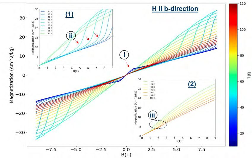
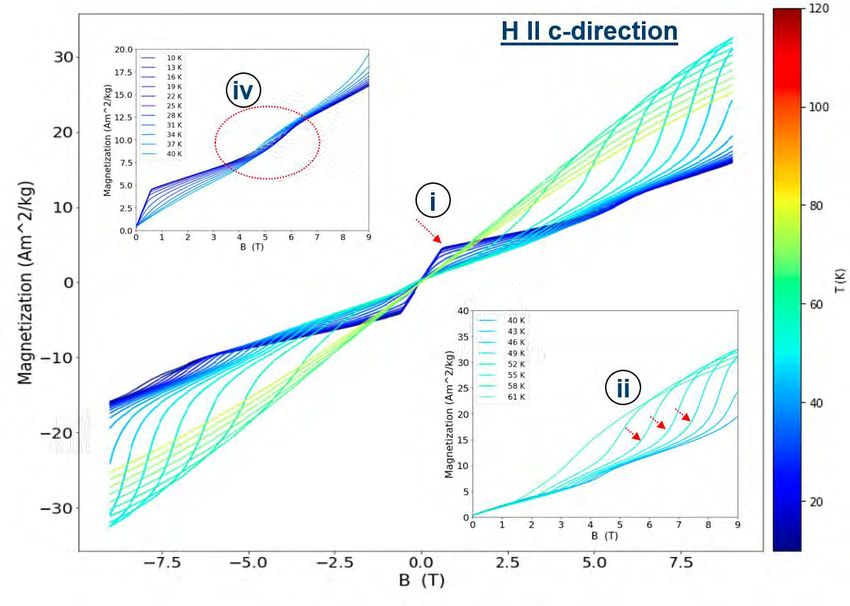
Abstract
Recently, the magnetocaloric effect (MCE) has been extensively studied theoretically and
experimentally, not only because of its potential for application in magnetic refrigeration
technologies, but also to gain a more solid understanding of the physical properties of the
materials. The magnetic refrigeration is a promising, energy-efficient technology and may be
an alternative to the conventional compression-expansion gas cycle refrigeration in the future,
as it has less environmental impact due to the fact that no greenhouse or ozone-depletion gases
have to be used.

The MCE is a thermodynamic phenomenon in which the magnetic entropy is changed in an
isothermal process, or the temperature of the material is changed in an adiabatic process, when
it is exposed to a magnetic field. There are two main quantities that characterize the MCE of a
material: the change in temperature in an adiabatic process ∆ , and the change in magnetic
entropy in an isothermal process ∆ .

Magnetocaloric 5 3 has received special attention with respect to its magnetic properties.
It shows two first-order transitions to two antiferromagnetic phases AFM1 and AFM2, at 66 K
and 99 K respectively. Another intermediate magnetic configuration AFM1 ´ occurs if a
magnetic field is applied, through which the compound transforms from the AFM1 phase to
the AFM2 state. Interestingly, the first magnetic transition around 99 K is associated with a
structural transition, at which the symmetry of the crystal structure changes from hexagonal to
orthorhombic. Moreover, this compound exhibits a less common type of MCE which is named
inverse MCE. This effect is associated with the phase transition between the two
antiferromagnetic phases AFM2-AFM1 where the spin arrangement changes from collinear to
non-collinear magnetic order.

In this thesis, the direction dependent macroscopic magnetic properties of a single crystal of
 5 3 were investigated using the Vibrating Sample Magnetometer (VSM) option. The mass
magnetization measurements were performed with the magnetic field applied along the three
different crystallographic directions a, b and c of the orthorhombic unit cell of the low
temperature structure. The magnetization measurements were performed for every sample
under two different protocols, the isothermal and the isofield conditions

Five main observations were obtained from field and temperature dependent magnetization
curves. (i) Low temperature-low magnetic field features were observed for application of the
field parallel to the orthorhombic base vectors

(ii) Features which are associated with the phase transition of AFM1´ - AFM2.

viii | P a g e

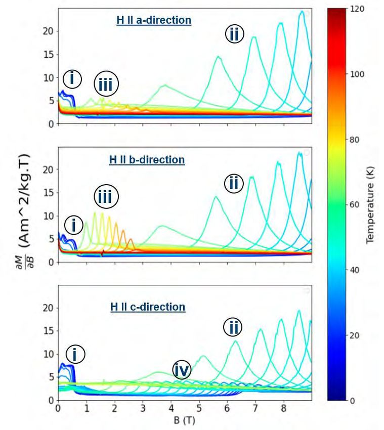
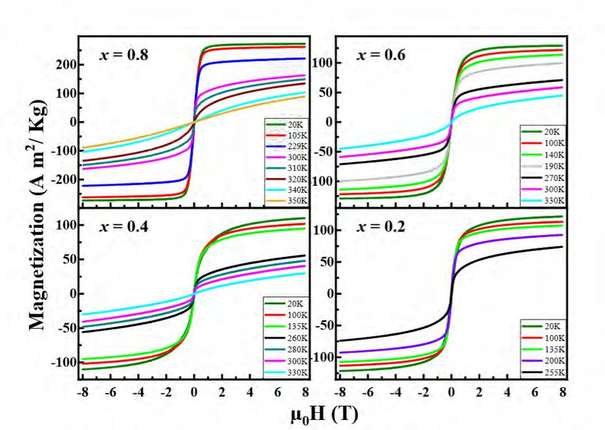
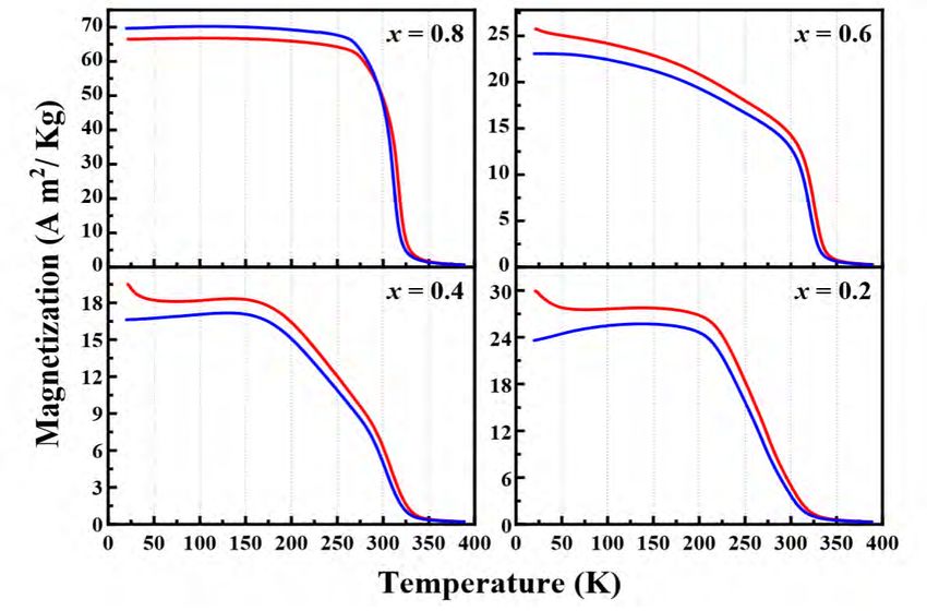
(iii) Features in the high temperature -low magnetic field region when the magnetic field is
applied in the ab-plane.

(iv) Features that can be attributed to the transition from AFM1 to the AFM1´ phase. These are
only observed when the magnetic field is applied parallel to the c-direction.

(v) Features corresponding to the transition from the PM phase to the AFM2 state. These can
only be observed, when small fields are applied || to the b-direction.

Based on these observations a field-temperature phase diagram could be obtained and it can be
concluded that the magnetic response of the sample is strongly affected by the direction of the
applied magnetic field. Our results show clearly that the magnetic response in the low
temperature phase AMF1 depends strongly on the field direction and is more complex than
previously thought. This complexity can most probably be mainly attributed to the existence
of two different crystallographic sites for the Mn ions within the crystal structure and the
mutual magnetic interactions between them.

Moreover, the magnetic entropy change ∆ of 5 3 was extracted based on Maxwell
relation between entropy/temperature and magnetization/field, which allows the calculation
from the field-dependent of the isothermal entropy change from magnetization data. The
compound exhibits an inverse MCE which corroborates the prevalence of AFM interactions.
A switch of the sign of magnetic entropy occurs around the transition temperature from the
non-collinear AFM1 to the collinear AFM2 phase. The maximum positive value of ∆ is
roughly 3.5 J/kg. K for a field change of 5.0 T at approximately 60 K.

Regarding the ( 5 3 ) ( 4 3 )1− compound in powder form, there was a doubt about
the reliability of earlier magnetization results for the sample with = 0.8 . According to the
earlier investigations, the saturation magnetization value exceeded 250 2 −1 at 20 K,
compared to the much lower saturation magnetization of approximately 100 2 −1 for
the other samples with = 0.6 , 0.4 , 0.2. To check this observation, a polycrystalline sample
of Mn4.2 Ge2.4 Fe0.8 Si0.6 was re-synthesized and x-ray powder diffraction was used to confirm
the phase purity of the compound. Afterwards, the magnetization was re-measured by
performing isofield measurements with two modes: field cooling (FC) and field warming (FW),
and isothermal measurements over a temperature range from 350 to 20 K. We find that the
saturation magnetization at 20 K is around 100 2 −1 as expected, and that evidently the
formerly reported value of 250 2 −1 is erroneous.

ix | P a g e

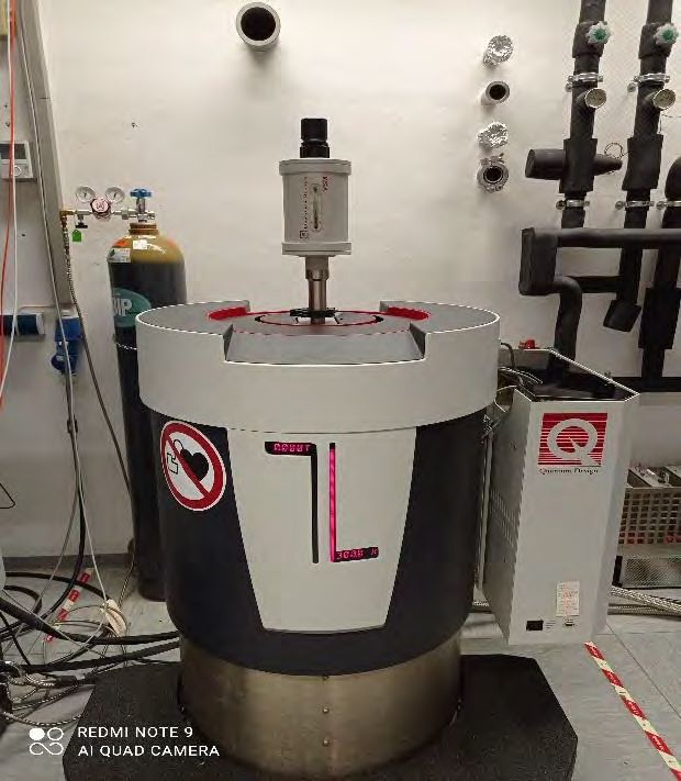
Table of contents
Declaration……………………………………………………………………………………v

Acknowledgments…...………………………………………………………………………vi

Place of experimental work………………………………………………………………...vii

Abstract…………………………………………………………………………………......viii

List of tables…………………………………………………………………………………xii

List of figures……………………………………………………………………………......xii

List of abbreviations……………………………………………………………………….xvi

1 Introduction................................................................................................... 1
 1.1 Motivation ......................................................................................................................................1

2 Theory ............................................................................................................ 3
 2.1 The magnetocaloric effect (MCE)..................................................................................................3
 2.1.1 History and definition ................................................................................................................3
 2.2 Thermodynamics of the MCE ........................................................................................................5
 2.3 Inverse MCE ..................................................................................................................................7
 2.4 Determination of MCE...................................................................................................................8
 2.4.1 Direct determination of MCE .....................................................................................................8
 2.4.2 Indirect determination of MCE ..................................................................................................9
 2.5 Scattering basics and diffraction techniques ..................................................................................9
 2.5.1 X-ray powder diffraction ..........................................................................................................11
 2.5.2 Laue single crystal diffraction ..................................................................................................11
 2.5.3 The Le Bail method ..................................................................................................................12

3 The magnetocaloric materials of this work .............................................. 14
 3.1 Introduction ..................................................................................................................................14
 3.2 The intermetallic compound 5 3 ...........................................................................................16
 3.2.1 Crystal structure of 5 3 ....................................................................................................16
 3.2.2 Magnetic structures of 5 3 ..............................................................................................18

 3.2.3 Summary of macroscopic magnetization measurements on 5 3 as described in the
 literature ..............................................................................................................................................20

4 Instrumentation .......................................................................................... 26
 4.1 Cold crucible induction melting device .......................................................................................26

x|Page

4.2 The MWL120 real-time back-reflection Laue camera .................................................................27
 4.3 Huber G670 powder diffractometer .............................................................................................28
 4.4 Vibrating sample magnetometer (VSM) of physical property measurement system (PPMS) .....29

5 Experimental procedures ........................................................................... 31
 5.1 Experimental part concerning 5 3 samples ...........................................................................31
 5.1.1 Sample preparation .................................................................................................................31
 5.1.1.1 Sample synthesis and single crystal growth ....................................................................31
 5.1.1.2 Laue diffraction experiment using MWL120 camera ......................................................31
 5.1.2 Magnetization measurements .................................................................................................33
 5.1.2.1 Iso-field magnetization measurements ...........................................................................33
 5.1.2.2 Iso-thermal magnetization measurements .....................................................................35
 5.2 Experimental part corresponding to the 4.2 2.4 0.8 0.6 sample .......................................36
 5.2.1 Sample preparation .................................................................................................................36
 5.2.1.1 Synthesis of the polycrystalline sample of 4.2 2.4 0.8 0.6 ....................................36
 5.2.1.2 X-ray powder diffraction using Huber G670 diffractometer ...........................................37
 5.2.2 Magnetization measurements .................................................................................................40
 5.2.2.1 Iso-field and iso-thermal magnetization measurements ................................................41

6 Data analysis (results and discussions) ..................................................... 42
 6.1 Laue diffraction of 5 3 single crystal samples ......................................................................42
 6.2 The LeBail refinement of 4.2 2.4 0.8 0.6 powder diffraction data ....................................46
 6.3 Magnetization measurements on 5 3 ....................................................................................49
 6.3.1 Magnetization measured under isofield conditions ................................................................49

 6.3.2 Magnetization measured under isothermal conditions ..........................................................53
 6.3.2.1 Magnetization measurements with H applied || to the a- and b-direction ...................53
 6.3.2.2 Magnetization measurements of H || c-direction ..........................................................58
 6.3.3 Characterization of the MCE ....................................................................................................64
 6.4 Magnetization measurements on 4.2 2.4 0.8 0.6 .........................................................68

 6.4.1 The previous work results ........................................................................................................68
 6.4.2 Results of the measurements performed in the course of this thesis .....................................70

7 Conclusions and Outlook ........................................................................... 72
 References …….………………………………………………………...76

xi | P a g e

List Of Tables
 page

 Table 3.1: Crystallographic data of . 16

 Table 6.1: The initial unit cell parameters and the parameters from the LeBail 48
 refinements of the patterns measured with the Huber diffractometer
 of 4.2 2.4 0.8 0.6 powder sample.

 Table 7.1: Summary of the main anomalies observed in the isothermal and 73
 isofield magnetization measurements that were performed on the
 single crystal of 5 3.

List Of Figures
 Chapter 2 page
 Figure 2.1: (left) The adiabatic magnetization, (right) The adiabatic 4
 demagnetization.
 Figure 2.2: S-T diagram of MCE. 6
 Figure 2.3: Bragg's Law is represented as schematic illustration. 10
 Figure 2.4: Schematic drawing of Debye-Scherrer cones. 12
 Chapter 3
 Figure 3.1: (left) Sketch of a magnetic phase diagram of the system 14
 5− 3 ( = 0,1,2,3,4,5), (right) The magnetic entropy
 change for a field change of 2T and 5T.
 Figure 3.2: 5 3 hexagonal unit cell projected along [001], green spheres 17
 represent Mn ions, red ones represent Si ions.
 Figure 3.3: Projection of the crystal structure of 5 3 a long [001]. The 17
 hexagonal unit cell and orthorhombic unit cell are presented with
 bold lines.
 Figure 3.4: The magnetic structure of 5 3 . (1) The collinear AFM2 Phase. 19
 (2) The non-collinear AFM1 phase. (3) The non-collinear AFM1´
 phase.
 Figure 3.5: Magnetic phase diagram of 5 3. 21
 Figure 3.6: Magnetic phase diagram of 5 3. 22
 Figure 3.7: Isothermal magnetization curves of 5 3 from (2-100) K. 23
 Figure 3.8: Isothermal magnetization curves of 5 3. , represents the 23
 magnetization values in the non-collinear and collinear phases
 respectively.
 Figure 3.9: The magnetic entropy change (−∆ ) of the 5 3 compound. 25

xii | P a g e

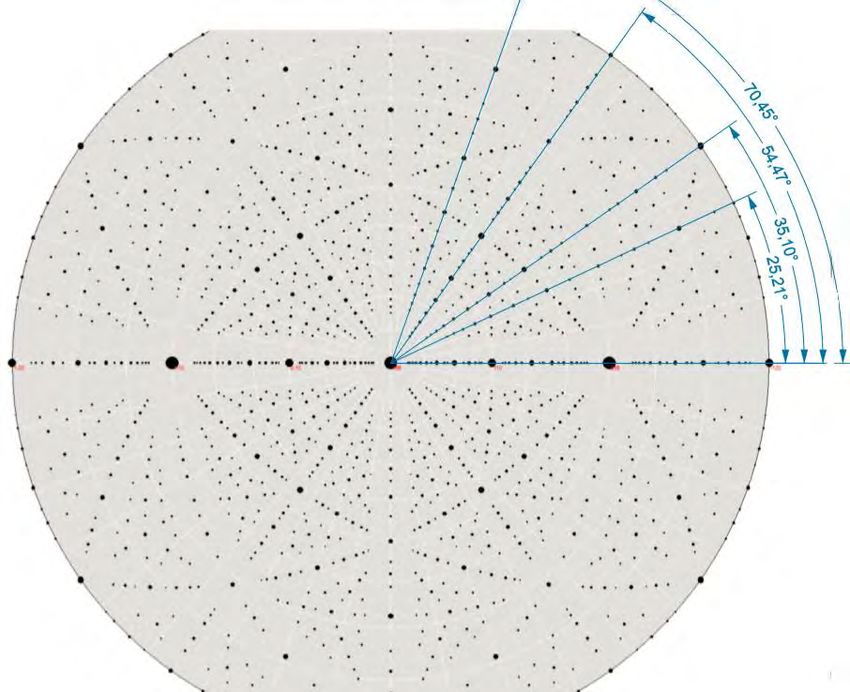
Chapter 4
 Figure 4.1: (left) Scheme of a cold crucible induction melting apparatus 26
 (Schematic view), (right) photo of the CCIM devise at the JCNS-2.
 Figure 4.2: (left) A sketch of the MWL120 camera, (right) A photo of the 28
 MWL120 camera at JCNS-2 which was used in this work.
 Figure 4.3: (left) Schematic view of the G670 diffractometer, (right) Huber 29
 G670 Powder Diffractometer at JCNS-2.
 Figure 4.4: (left) Schematic View of VSM option, (right)PPMS Dynacool at 30
 JCNS-2.
 Chapter 5
 Figure 5.1: (a) Fixing the sample on the holder. (b) Inserting the holder inside 32
 the MWL120 Laue camera. (c) The samples cut with spark erosion.
 (d) An image for 5 3 single crystal along [001] axis obtained
 from the Laue camera. (e) The three oriented samples of 5 3
 along [100], [1-20] and [001] axis.
 Figure 5.2: (a) Fixing the sample on the holder at a specific location using the 35
 mounting station, the red arrow is pointing to the sample. (b) The
 sample after Teflon covering. (c) The dialogue for the sample
 centering scan.
 Figure 5.3: (left) The containers of the high purity elements of , , , , 37
 (right) Cold Crucible Induction Melting device, (right) The glowing
 sample is visible.
 Figure 5.4: (a) Polycrystalline sample as obtained from CCIM. (b) Crushed 38
 sample inside a mortar. (c) Final fine homogamous powder of
 4.2 2.4 0.8 0.6 compound.
 Figure 5.5: (left) Powder sample inserted in sample holder to be used in x-ray 39
 diffraction experiment, (right) The Huber G670 diffractometer
 system in JCNS-2.
 Figure 5.6: Trough-shaped holder in which the capsule of the sample is inserted, 41
 the red arrow is pointing to the sample.

 Chapter 6
 Figure 6.1: (top) The calculated stereographic projection based on the lattice 43
 parameter from an 5 3 single crystal along the [100] direction
 as obtained from the OrientExpress 3.4 program. (bottom) The real-
 time Laue camera image along the same crystallographic direction.
 Figure 6.2: (top) The calculated stereographic projection based on the lattice 44
 parameter from an 5 3 single crystal along the [120] direction
 as obtained from the OrientExpress 3.4 program. (bottom) The real-
 time Laue camera image along the same crystallographic direction.

xiii | P a g e

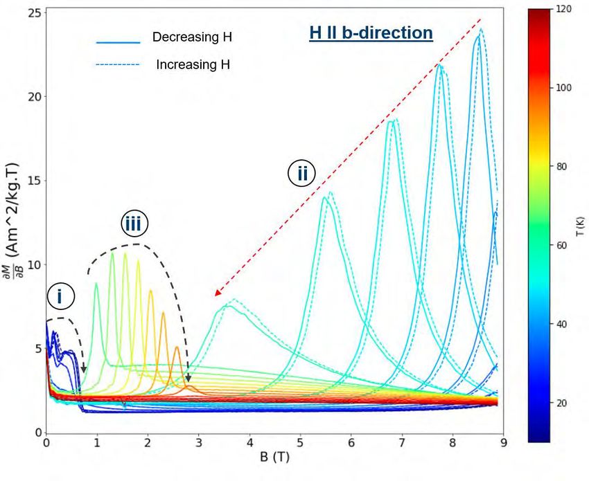
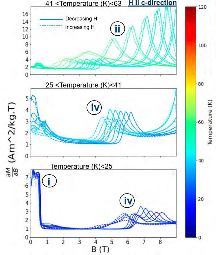
Figure 6.3: The real-time Laue camera image along the [001] direction of 45
 5 3 .
 Figure 6.4: The LeBail fit of the room temperature data of 4.2 2.4 0.8 0.6 47
 using two phases and the resulting difference profile from Jana2006.
 Figure 6.5: Molar magnetic susceptibility of 5 3 single crystal with fields 50
 of varying strength applied along the different crystallographic
 directions.
 Figure 6.6: (top) The isofield magnetization curves M(T) of the three 52
 crystallographic directions, at H = 1.5 T and at H = 7.5 T (bottom).
 Figure 6.7: The field-dependent magnetization curves (M(B)) of 5 3 . 54
 Decreasing H data, H || b-direction, in the temperature range
 10 K - 120 K.
 Figure 6.8: The first derivative of the M(B) curves, ( ⁄ ) vs. ( ). 55
 Figure 6.9: ( ⁄ ) for the magnetization data of 5 3 single crystal as a 57
 function of applied magnetic field and temperature, H || b-direction.
 Shades of red and blue represent the positive and negative
 ( ⁄ ) of the sweeping down data respectively.
 Figure 6.10: The field-dependent magnetization curves (M(B)) of 5 3 . 59
 Decreasing H data, H || c-direction, in the temperature range
 10 K - 76 K.
 Figure 6.11: The ( ⁄ ) vs. ( ) curves of 5 3 , H || c − direction, for 60
 three temperature ranges, (bottom) T

Figure 6.17: Isothermal magnetization measurements of the compounds in the 69
 system ( 5 3 ) ( 4 3 )1− . Full hysteresis measurements
 (±8 ) are shown.
 Figure 6.18: Field-dependent magnetization data of a polycrystalline sample of 70
 4.2 2.4 0.8 0.6 in the temperature range from 350 K
 to 20 K.
 Figure 6.19: Temperature-dependent magnetization data of a polycrystalline 71
 sample of 4.2 2.4 0.8 0.6 at a magnetic field setting
 of 0.1 T.
 Chapter 7
 Figure 7.1 The ( ⁄ ) vs. ( ) curves for the a, b, and c-direction. 74

xv | P a g e

List Of Abreviations
 Abbreviation Representation
 MCM Magnetocaloric material
 MCE Magnetocaloric effect
 AFM Antiferromagnetic
 FIM Ferrimagnetic
 PM Paramagnetic
 FM Ferromagnetic
 Curie Temperature
 Néel temperature
 SOPT Second order magnetic phase transition materials
 FOPT First order magnetic phase transition materials
 ∆ Adiabatic temperature change
 S Entropy
 C Heat capacity
 ∆ Magnetic entropy change
 ∆ Isothermal entropy change
 Lattice entropy
 Electronic entropy
 T Absolute temperature
 H Magnetic field strength
 B Magnetic flux density
 M Magnetization
 0 Magnetic permeability of free space
 Bohr magneton
 Oe Oersted
 Mn Manganese
 Si Silicon
 Wavelength
 FWHM Full width at half maximum parameter
 Profile R-factor
 Weighted profile R-factor
 CCIM Cold crucible induction melting
 PPMS Physical properties measurement system
 VSM Vibrating sample magnetometer
 χ Molar magnetic susceptibility

xvi | P a g e

1 Introduction
1.1 Motivation

Recently, the magnetocaloric materials (MCM) are gaining more attention due to their
promising magnetocaloric effect (MCE) in which the magnetic entropy of the material
is changed when it is exposed to a magnetic field. The potential of MCE is the base of
magnetic refrigeration which is considered as an efficient and environmentally friendly
cooling and temperature control system [17].

 5 3 has received special attention with respect to its magnetic properties. At room
temperature (300 K) the compound is found to be in a paramagnetic state and
crystallizes in a hexagonal structure type 88 with space group ( 63 / ) [18].
During cooling, the compound behaves unusually concerning the structural and
magnetic transformations [19]. It shows two first-order transitions to two
antiferromagnetic phases AFM1 and AFM2 [20], at 66 K and 99 K respectively.
Moreover, the first magnetic transition at 99 K is associated with a structural phase
transition at which the symmetry of the crystal structure is changed from hexagonal
with unit cell parameters, ℎ = 6.910 Å , ℎ = 4.814 Å , = 2 [21], to face centered
orthorhombic symmetry with space group , and lattice parameters =
6.89856(1), = 11.9120(2), = 4.79330(1)Å , = 4 [22]. Another intermediate
magnetic configuration AFM1´occurs if a magnetic field is applied, through which the
compound transforms from the AFM1 phase to the AFM2 state. The magnetic
structure of 5 3 at low temperatures is somehow complicated and unusual.

This compound exhibits a less common type of MCE which is named inverse MCE,
where the material cooled down when exposed to a magnetic field in the context of
adiabatic process (∆ < 0), while ∆ > 0 or in other words, the magnetic entropy
is increased while the material is exposed to an external magnetic field [17].

Concerning 5 3 , the inverse MCE is associated with the phase transition between
the two antiferromagnetic phases where the spin arrangement changes from collinear
to non-collinear magnetic order [23]. Moreover, topological anomalous Hall effect was
observed in the non-collinear AFM phase, which can potentially be used to develop
new storage or computational devices [13, 24, 25].
1|Page

In this thesis, the macroscopic magnetic properties of 5 3 compound in the form
of single crystal were investigated by direction dependent magnetization
measurements, and the MCE has been characterized as well.

On the other hand, I will present mass magnetization measurements on
( 5 3 ) ( 4 3 )1− for a value of ( = 0.8) . The quasi-binary system
( 5 3 ) ( 4 3 )1− , was already investigated with x-ray powder diffraction and
macroscopic magnetic properties in the course of a previous master thesis of K. Al-
Namourah [9]. According to the observations described there, for ( 4.2 2.4 .8 .6)
in which ( = 0.8) the saturation magnetization value was doubled compared to other
samples of the series ( = 0.6 , 0.4 , 0.2 ). This observation was surprising and – if true
– would potentially have been of importance for an application of the material.
Therefore, there was a strong reason to reproduce the measurements for this sample.

2|Page

2 Theory
2.1 The magnetocaloric effect (MCE)

2.1.1 History and definition

The MCE is considered to be a magnetic thermodynamic phenomenon in which the
magnetic entropy is changed in an isothermal process, or the temperature of the
material is changed in an adiabatic process, when it is exposed to a magnetic field
[14].

The German physicist Warburg had noticed the MCE 140 years ago [26] , followed
by Weiss [27]. The basic principle of the MCE was introduced by P. Debye in 1926
and W. Giauque in 1927 [28].The MCE is the basis of magnetocaloric refrigeration
technology, which depends on magnetocaloric materials exhibiting an MCE ideally
near to room temperature. The first highly efficient environmentally friendly magnetic
refrigerator was built in 1933 and was based on the adiabatic demagnetization of
paramagnetic salts adiabatically to reach a very low temperature (< 0.5 ) [29] . A
series of different designs and research investigation on this promising technology
have followed over the years [17] .

For a simple ferromagnetic material near its Curie temperature ( ), randomly oriented
magnetic moments are aligned in an ordered way when the magnetic field is activated.
This leads to a decrease in the magnetic entropy while increasing the lattice entropy
and heating up the material. If the magnetic field is removed, then the magnetic
moments return to be randomly oriented. This increases the magnetic entropy and to
compensate the material cools down [30] (Fig.2.1) .

The applicable magnetocaloric materials (MCM) can be classified into second order
magnetic phase transition materials (SOPT) and first order magnetic phase transition
materials (FOPT). The classification depends on the type of transition the material
undergoes between the ferromagnetic and paramagnetic state. For SOPT materials,
the magnetization changes continuously with changing the temperature, while for
FOPT materials, the change in magnetization is discontinuous as a function of
temperature. The rare earth metal Gd is a prototype of a material that undergoes

3|Page

SOPT [31], with low thermal and magnetic hysteresis. 5 2 2 [32] on the other
hand, is a typical FOPT magnetocaloric material with a giant MCE, as the magnetic
transition is associated with a structural phase transition. One of the drawbacks of
FOPT materials is the high thermal and magnetic hysteresis compared to SOPT
materials.

Most of the research these days focus on the application of MCM that can be utilized
e.g., in highly efficient magnetic refrigerator, and hence the research is strongly related
to devices engineering and materials science. However, a lot still remains unknown
about the mechanism of the MCE and its worthwhile to perform research in this
direction to enrich our knowledge about the phase transitions and thermomagnetic
characteristics of the materials. Hence, there are many compounds where the
observed magnetocaloric properties are not appropriate for potential refrigerants, but
still the investigation of the MCE in them is a suitable tool to determine and
understand the underlying principles of the MCE [33] .

 Fig.2.1 (left) The adiabatic magnetization, (right) The adiabatic demagnetization [10].

4|Page

2.2 Thermodynamics of the MCE

There are two main quantities that characterize the MCE of a material: the change in
temperature in an adiabatic process ∆ , and the change in magnetic entropy in an
isothermal process ∆ .

If the pressure is constant, the total entropy (S) of a material is a function of
temperature (T) and the applied magnetic field (H). The overall entropy of the MCM is
the sum of three contributions: the lattice entropy as a function of temperature ( )
the magnetic entropy as a function of T and H ( , ) , and the electronic entropy
as a function of T ( ).

 ( , ) = ( , ) + ( ) + ( ) (1)

As for the lattice and electronic entropy , , respectively, they are functions of the
absolute temperature (T) and independent of the magnetic field (H), while the
magnetic entropy ( , ) is highly dependent on (H). The MCE of all magnetocaloric
materials result from the coupling of the magnetic field effect with the magnetic sub-
lattice.

Fig.2.2 illustrates the two parameters that can represent the MCE of a ferromagnetic
material, ∆ and ∆ where the x-axis represents the temperature of the material,
while the y-axis represents the total entropy of the material. Around the material
shows its maximum MCE [34] .

The dashed lines represent the magnetic entropy when the magnetic field is zero
( 0 = 0) and when it is at any value larger than zero ( 1 > 0.0), the third dashed line
represents the sum of ( + ), while the solid lines show the total entropy ( ) when
the magnetic fields are 0 , 1 , respectively.

If a magnetic field is applied ( 1 ) adiabatically (reversible adiabatic magnetization),
then the magnetic entropy is decreased while the overall entropy is constant and
the solid is heated up [30]. In other words, to maintain ( 0 , 0 ) = ( 1 , 1 ) the lattice
entropy is increased. Under this adiabatic process, the MCE of the material is
represented by the change in adiabatic temperature as ∆ = 1 − 0 .

5|Page

Fig.2.2 S-T diagram of MCE [7].

If the magnetic field is applied under isothermal conditions (at constant temperature
( 0 )), the magnetic entropy is decreased, as a consequence the total entropy is
decreased too. The MCE is given by the change in magnetic entropy:

 ∆ = ( 0 , 0 ) − ( 0 , 1 ) (2)

Depending on Maxwell’s relation [35], ∆ and ∆ could be calculated:

 ( , ) ( , )
 ( ) =( ) (3)
 
where, H: magnetic field, T: temperature, M: magnetization, S: entropy.

By integrating both sides of Eq. 2 and regarding the isothermal process at constant
pressure, it follows:
 2
 ( , )
 ∆ ( , ∆ ) = ∫ ( ) (4)
 1 

 ( , )
The previous equation states clearly that the greater the ( ) the greater the
 
MCE. The peak of MCE occurs around the phase transition temperature.

In adiabatic process, the infinitesimal adiabatic temperature rise is obtained from
combining equation (2) and ( = = − ), Q is the heat flux and C is the heat
capacity. Which gives:

6|Page

 ( , )
 = − ( ) ( ) (5)
 ( , ) 

By integrating Eq.4, it will give a quantitative value for ∆ :
 2
 ( , )
 ∆ ( , ∆ ) = − ∫ ( ) ( ) (6)
 1 ( , ) 

where, ( , ) is the heat capacity of the MCM.

It becomes clear from the previous equation that the MCE can be improved by a wide
field variation, and/or by choosing MCM with small heat capacity, and/or greater
 ( , )
( ) .
 
The question now is: how to calculate the ∆ and /or ∆ practically? In the context
of next sections, a brief description about the determination of MCE will be provided.

2.3 Inverse MCE

It is clear that there is a strong relationship between the entropy of the system which
is associated with structural and magnetic changes and the size of MCE. According to
what has been mentioned previously, there are two main quantities that characterize
the MCE of a material: the change in temperature in an adiabatic process ∆ , and
the change in magnetic entropy in an isothermal process ∆ . In regular MCE
materials, the sample heats up when exposed to a magnetic field adiabatically, which
means that ∆ > 0, while during the isothermal process, the instantaneous change
of magnetization with respect to instantaneous change of temperature is negative
∆ < 0. Effects obeying these characteristics are named traditional or direct MCE [1].
The opposite case, that is the temperature derivative of the magnetization is positive,
and the sample cooled down when exposed to a magnetic field in the context of
adiabatic process (∆ < 0), while ∆ > 0 or in other words , the magnetic entropy
is increased while the material is exposed to an external magnetic field , this is the
inverse MCE [17].

Although the inverse MCE is more rarely investigated than the direct one, it is found
in many magnetic systems, in particular when antiferromagnetic order is involved.

7|Page

Examples include: the magnetic transition from anti-ferromagnetic to a ferrimagnetic
phase (AFM/FIM) like in 1.82 0.18 [36], or the transition from collinear anti-
ferromagnetic to non-collinear anti-ferromagnetic phase like in 5 3 [14], or the
anti-ferromagnetic to ferromagnetic phase (AFM/FM) as observed in 0.49 ℎ0.51 [37].

According to earlier investigations, the inverse MCE can be explained by the fact that
the application of an external magnetic field induces spin fluctuations, which leads to
an increase of the magnetic entropy [14, 38].

2.4 Determination of MCE

There are two different methods to measure the magnetocaloric effect: the direct
measurements and the indirect ones. The direct method requires measurement of the
samples temperature while applying and removing a magnetic field in an adiabatic
process. On the other hand, the indirect method is based on the measurement of
magnetization as a function of magnetic field and temperature.

2.4.1 Direct determination of MCE

The MCE could be obtained directly by measuring 0 at 0 and 1 at 1 under
adiabatic conditions with an error ratio 5-10% which depends on the quality of the
thermal insulation of the sample, the accuracy of the thermometer and the strategy
that is followed to prevent the thermal sensor readings from being affected by the
changes in magnetic field [7].

The adiabatic process is fulfilled if it is assured that no heat is exchanged, in practice
this can be achieved by rapid changes of the magnetic field. So, if e.g. the material is
moving at a specific speed through a fixed magnetic field or the magnetic field is
moved at a certain speed while the material remains fixed, then we will ensure that the
adiabatic conditions are met [30, 39].

8|Page

2.4.2 Indirect determination of MCE

The indirect measurements of the MCE could be achieved by two methods, one is the
calorimetric method which relies on the heat capacity of the material to calculate both
∆ ( , ∆ ) and ∆ ( , ∆ ) , the other one is the magnetization method which
calculates ∆ as function of temperature and magnetic field.

∆ ( , ∆ ) is the most commonly used parameter to characterize the MCE [40]. It can
be calculated from the isothermal magnetization curves or isofield magnetization
curves. Numerically, integrating Eq.3 will produce a quantitative value of ∆ [41] .

The error ratio of ∆ which is obtained from the magnetization measurements is 3-
10%, where the accuracy of the result depends on temperature, magnetic moment
and field measurements.

It should be pointed out that, regardless of the methods that are used to characterize
the MCE, the results should not be completely divergent or equal, but rather
convincingly close. Both quantities of |∆ | and |∆ | depend on ( 0 ) and the
difference between the initial and the final field ( 1 − 0 ).

Experimentally, it is easier and faster to sweep the magnetic field continuously
(stabilizing H at different values) than sweeping the temperature of the material at a
ramp rate (stabilizing T at different values), in particular if one takes into account the
time needed for a measurement [42].

In this thesis, indirect measurements were performed to characterize the MCE of
 5 3 in the form of single crystal. ∆ ( , ∆ ) was calculated via isothermal
magnetization curves and/or isofield measurements.

2.5 Scattering basics and diffraction techniques

Scattering techniques are used to obtain detailed information about the crystal
structure of a material at the microscopic level. In particular, X-ray diffraction is an
analytical non-destructive elastic scattering method used to get structural information

9|Page

of the materials [43]. If one compares the wave length of the X-rays with the inter-
atomic distances in the crystals, they are approximately similar (~ .15 − .4 ). This
means that X-rays are a very appropriate choice to perform diffraction experiments on
crystalline materials [44].

In crystals, when electromagnetic radiation hits parallel lattice planes spaced apart by
an interplanar distance , the incoming wave will be scattered. if the difference
between the path lengths of the diffracted beams from a neighboring lattice planes is
an integer multiple of the incident wavelength, the scattered waves are in phase. This
condition was defined by Lawrence Bragg, and it is described by Bragg’s equation
[43]. Bragg's law [6] describes the conditions at which constructive interference
between the scattered waves occurs, (see Fig.2.3) , that is:

 = 2 sin (7)

where : is the order of diffraction (a positive integer), : the wavelength, : the
distance between two parallel lattice planes ( ℎ ), : the glancing diffraction angle.

The previous relationship is the basis for a diffraction experiment where the diffracted
intensity is recorded as a function of the diffraction angle.

 Fig.2.3 Bragg's Law is represented as schematic illustration, taken from Ref. [6].

In this thesis Laue diffraction was used to define the correct crystallographic
orientation of the single crystals of 5 3 for the magnetization measurements and

10 | P a g e

X-ray powder diffraction was used to check the phase purity of the polycrystalline
material of 4.2 2.4 .8 .6. The basic concepts of the two diffraction methods will
be explained in the next section.

2.5.1 X-ray powder diffraction

x-ray powder diffraction is a non-destructive technique which uses X-ray radiation on
polycrystalline samples to characterize the structure of the material. It is also used in
quantitative phase analysis or for tracking of phase transitions under the influence of
temperature , pressure , and magnetic or electrical fields [6] . Powder samples can be
considered as ideal if a large number of crystallites exists where all possible
orientations of a crystal lattice exist in equal proportions.

In an X-ray powder diffraction experiment, a beam of monochromatic X-ray radiation
hits the powder sample. As the crystal lattice in the powder has all possible
orientations, one will observe all the possible diffraction peaks from lattice planes for
which the Bragg condition is fulfilled. Peaks with identical Bragg angles form cones
which are called Debye-Scherrer cones. Every Debye-Scherrer cone is related to a
single set of lattice planes. In a flat plate detector, these cones will be projected as a
2-D image of smooth concentric rings. Usually, the diffraction patterns are presented
by a diffractogram in which the intensity ( ) is represented as a function of the
scattering angles (2 ) (Fig.2.4) [44].

2.5.2 Laue single crystal diffraction

In this work, Laue diffraction was employed to define the crystal orientation of a single
crystal of 5 3 . For the Laue method a polychromatic beam is used. In other words,
multiple wavelengths are used to irradiate the fixed single crystal sample. This means
that the incident angle and the incoming beam have a specific orientation with
respect to individual lattice planes (ℎ ) . If Bragg’s law is satisfied for a particular

11 | P a g e

lattice plane and a specific wavelength, constructive interference occurs. In this case
the detector will record a diffraction spot [45].

 Fig.2.4 Schematic drawing of Debye-Scherrer cones, taken from Ref. [6]

2.5.3 The Le Bail method

The Le Bail method is a technique used to fit the measured powder diffraction pattern
to a calculated one which follows from an assumed model. With this method the unite
cell parameters of the crystal structure can be determined, and an initial idea about
the space group of the crystal structure can be obtained. For this, an algorithm which
depends on an iterative least squares analysis is used [46]. In addition to refining the
unit cell parameters, many other parameters could be refined e.g., the background,
the profile function, and the zero-shift parameter.

As an initial step in this method, approximate values of unite cell parameters and an
initial space group of the crystal structure are provided. Using this primary input, the
diffraction patterns diagram is calculated and then compared to the measured one.
Then one starts adjusting the mentioned parameters (unit cell parameters, background
parameters, profile function and zero shift parameter) to reduce the difference
between the measured and calculated diagrams. In the next step, a new diffraction

12 | P a g e

diagram is calculated and the processes of comparing, adjusting and calculating
another new diffraction diagram is repeated, until a satisfactory agreement between
the measured and the calculated diagrams is reached. Numerical criteria are used to
quantify the agreement. These are: the profile R-factor ( ) and the weighted profile
R-factor ( ),

 ∑ | , − , |
 = (8)
 ∑ , 

where, , : observed intensity at a specific diffraction profile point, , :
calculated intensity at a specific diffraction profile point.

 ∑ ( , − , )2
 =√ (9)
 ∑ , 2

where, : weighting factor = 1⁄ .

 is a well-known indicator that expresses the quality of the refinement. In practice
many programs are available which use the Le Bail technique like e.g. BGMN [47] ,
ARITVE [48], FullProf [49], Jana2006. In this thesis Jana2006 [50] is used .

13 | P a g e

3 The magnetocaloric materials of this work
3.1 Introduction

The Pseudo binary system 5− 3 with ( = 0,1,2,3,4,5) has MCE at different
temperatures depending on the different values of ( ). The parent structure of all
compounds in the system crystalizes in a hexagonal structure with space group
( 63 ⁄ ) [51]. Mn and Fe ions occupies two different crystallographic sites, 6(g)
and 4(d) respectively, the occupation ratio depends on the compositional ( )
parameter [52].

The magnetocaloric properties and the magnetic transitions in this system was
investigated by [16], using magnetization measurements as a function of magnetic
field and temperature. At low temperatures the Mn-rich compounds ( = 0,1,2) shows
two different antiferromagnetic phases (AFM1, AFM2). It was found that, the
temperature of antiferromagnetic ordering shifts to higher temperature, as the
parameter ( ) is increasing, in another word, as increasing the ratio of Fe. For Fe-rich
compounds ( = 4,5) ferromagnetic order was observed (Fig.3.1, (left)).

 Fig.3.1 (left) Sketch of a magnetic phase diagram of the system − ( = , , , , , ),
 (right) The magnetic entropy change for a field change of 2T and 5T. Figure taken from [16].

14 | P a g e

The compound 4 3 ( = 4) crystalizes in space group − 6 with lattice
parameters = 6.8054(7) Å and = 4.7290(5) Å [53]. It shows the largest
magnetocaloric effect compared to the other compounds in this system (Fig.3.1,
(right)) at a transition temperature around room temperature ( = 300 ) where it
changes from a paramagnetic to a ferromagnetic phase. The closely related
compound 5 3 , which crystalizes in the same structure type (space group
 63 ⁄ , and cell’s dimensions = 7.184(2)Å, = 5.053(2)Å) [54], also shows a
ferromagnetic transition at a similar temperature ( = 304 ) . Around ( ), this
compound shows a second order transition phase with considerably larger MCE, as
the magnetic entropy change is about (3.8) (9.3) ⁄ . at field change of 2.0
and 5.0 T respectively [23]. In addition to a rapid change in magnetization [23]. This
compound would therefore be more suitable for applications than 4 3 , yet there
is a limitation which decreases the usage of this compound on a large scale, due to
the high content of the rather expensive element Ge.

As both compounds crystallize in the same structure type and show MCEs at similar
temperatures, it is interesting to look at the properties of the quasi-binary solid solution
of 4 3 and 5 3 . This quasi-binary system ( 5 3 ) ( 4 3 )1− ,
contains mainly (Mn, Fe, Si) which are abundant, non-toxic, and non-expensive
elements. The potential of the magnetocaloric effect was already investigated with x-
ray powder diffraction and macroscopic magnetic properties in the course of a
previous master thesis of K. Al-Namourah [9]. In this thesis, I will present the repetition
of mass magnetization measurements of ( 5 3 ) ( 4 3 )1− for a value of ( =
0.8), the motivation for this repeating this investigation will be discussed later on.

Going back to the system 5− 3 , there is another remarkable compound which
is one of the end members, 5 3 ( = 0). This compound exhibits two well-known
antiferromagnetic phase transitions and inverse MCE at low temperature. More deep
details about this intermetallic compound will be provided in the next section.

In short, in this thesis I worked on two different compounds which are: 5 3 single
crystal compound and a polycrystalline sample of 4.2 2.4 .8 .6 . The DC-field
mass magnetization measurements with different protocols were performed on both
of them to investigate the macroscopic magnetic properties and to calculate the
potential of the MCE.

15 | P a g e

3.2 The intermetallic compound 

3.2.1 Crystal structure of 

At room temperature (300 K) the compound is found to be in paramagnetic state and
crystalizes in a hexagonal structure type 88 with space group ( 63 / ) [18] , with
unit cell parameters, ℎ = 6.910 Å , ℎ = 4.814 Å , = 2 [55] . The atomic positions of
this structure were first determined by Aronsson in 1960 [21] and later confirmed by
Lander and Brown in 1967 [22]. Table (3.1) contains more detailed crystallographic
data on the compound.

 Table (3.1) Crystallographic data of [22].

 Space group: 63 ⁄ , = 2

 At 300 K, unit cell parameters: ℎ = 6.910 Å , ℎ = 4.814 Å

 Atomic positions site symmetry

 (4) Mn1 in 4(d) ±( 13 , 23 , 0) ;( 23 , 13 , 12 ) 32

 (6) (Mn2 in 6(g) ±( , 0 , 14 ); (0 , , 41 ); (− , − , 14 ) = .2360(1) mm

 (6) Si in 6(g) ±( , 0 , 14) ; (0 , , 14 ); (− , − , 14 ) = .5991(2) mm

Fig.3.2 shows the projection of the crystal structure of 5 3 along [001] that was
proposed by [56]. The hexagonal unit cell is displayed and the different atomic
positions of Mn1, Mn2 and Si atoms are shown. Manganese ions occupy two different
crystallographic sites, namely 4(d) which is occupied by Mn1 ions and 6(g) that is
occupied by Mn2 ions [55].

16 | P a g e

Fig.3.2 hexagonal unit cell projected along [001], green spheres
 represent Mn ions, red ones represent Si ions, taken from [1] .

The low temperature (4.2 K ) structure of 5 3 was first studied by [22] before more
than 50 years ago. At low temperatures, the compound undergoes a structural phase
transition at which the crystal structure is changed to orthorhombic unit cell with lattice
parameters = 6.89856(1), = 11.9120(2), = 4.79330(1)Å . The lattice
parameters of orthorhombic unit cell could be represented with respect to those of the
hexagonal unit cell as ℎ ≈ , ℎ ≈ and √3 ℎ ≈ , Fig.3.3 shows the projection
of the structures along [001] and illustrates the relation between the hexagonal unit
cell and the orthorhombic one.

 Fig.3.3 Projection of the crystal structure of a long [001]. The hexagonal unit cell and
 orthorhombic unit cell are presented with bold lines. The figure taken from [15].

17 | P a g e

3.2.2 Magnetic structures of 

During cooling, the compound 5 3 behaves in an unusual way and exhibits
structural and magnetic transformations [19, 20]. When the compound is cooled down
to Néel temperature 2 ≈ 99 , a magnetic transition from the paramagnetic phase
(PM) to a collinear antiferromagnetic phase (AFM) is observed. This magnetic phase
is known as AFM2 [1, 11, 15, 22, 57, 58]. As cooling continues down to 1 ≈ 66 
another transition takes place from the AFM2 to a non-collinear antiferromagnetic
phase which is known as AFM1 [20] .

The first magnetic transition at 2 is associated with above-described change in the
crystal structure, where the symmetry is reduced to a face centered orthorhombic
phase with space group and = 4.

In the AFM2 phase, only two third of the Mn2 ions have an ordered magnetic moment
of = 1.5 . Spins are arranged in a collinear style and aligned parallel and
antiparallel with respect to the b-axis of the orthorhombic unit cell (see Fig.3.4 (1)).
The Mn1 ions and the remaining one third of Mn2 show no ordered magnetic moments.
This implies that, the Mn2 ions are not symmetry equivalent any more but split into two
independent sets [1, 15, 56]. Mn21 atoms occupying Wyckoff positions 4(c) with site
symmetry (mm) and Mn22 atoms on Wyckoff positions 8(g) with site symmetry (m).
As illustrated before, only Mn22 atoms exhibits an ordered magnetic moment.

In the AFM1 phase, the magnetic moments re-oriented to different directions in a
highly non-collinear fashion. One third of Mn2 atoms still does not show an ordered
magnetic moment, yet in contrast to this the atoms on the Mn1 do develop an ordered
moment. This fact has been related to the expansion of the crystallographic c axis at
the AFM2-AFM1 transition which leads to an increased distance between the Mn1
atoms [56]. This increased distance is above the critical distance for magnetic ordering
on the Mn-ions (Fig.3.4 (2)).

18 | P a g e

Fig.3.4 The magnetic structure of . (1) The collinear AFM2 Phase. (2) The non-collinear AFM1
 phase. (3) The non-collinear AFM1´ phase [12]. (View along the c-direction)

Below 66 K (AFM1), the symmetry of the crystal structure is still orthorhombic, yet the
atoms occupying the Mn22 sites are magnetically different. They split into two parts,
Mn23 and Mn24. In reference [56], the AFM1 was investigated at 4.2 K with single-
crystal neutron diffraction and zero-field neutron polarimetry, and it was shown that
atoms of Mn1 exhibit ordered moments of = 1.20(5) oriented parallel and anti-
parallel to the direction with polar coordinates = 105(1)°, = 116(1)° , where is
measured from [010] and from [001] axis. Still Mn21 exhibits no ordered magnetic
moment, but Mn23 exhibit magnetic moment of = 2.30(9) with polar coordinates
 = 93(1)° , = 70(1)° , while Mn24 atoms exhibit a different value of magnetic
moment of 1.85(9) oriented to the directions with polar coordination of = 11(7)°
and = 21(1)° .

According to all these observations, the magnetic structure of 5 3 at low
temperatures is complex and unusual, as the atoms exhibit different magnetic
moments even, they have similar chemical environments.

In addition, Sürgers et al. [13] observed an intermediate magnetic configuration which
occurs if a magnetic field is applied. This phase was named AFM1´, and represents a

19 | P a g e

state through which the compound transforms from the AFM1 phase to the AFM2
phase. In this intermediate transition, a non-collinear phase was suggested as well,
however with a different spin arrangement compared to the AFM1 phase (Fig.3.4(3)).

The inverse magnetocaloric effect (Inverse MCE) is an effect which coincides with the
transition from the collinear AFM2 to the non-collinear AFM1. At this transition, the
sign of ∆ changes around 1 from negative to positive [16]. As mentioned before,
following Maxwell’s thermodynamic relationship ( ⁄ ) = ( ⁄ ) , cooling can
be obtained if a sample that was isothermally magnetized before is adiabatically
demagnetized. In the AFM1 phase, cooling can be obtained through adiabatic
magnetization [17].More details about what is known in the literature about this effect
in 5 3 will be provided in the next section.

3.2.3 Summary of macroscopic magnetization measurements on 
 as described in the literature

Many experimental studies were carried out to investigate the physical characteristics
and magnetic properties of 5 3 due to the attractiveness of its unusual magnetic,
structural and magneto-functional properties.

A single crystal of 5 3 compound grown by Czochralski method was
experimentally investigated in [57]. Static magnetic fields of up to 15 T was applied
parallel to the hexagonal axis (H ll c). Besides the two well-known first-order
transitions, an additional magnetic transition associated with hysteresis was observed
in the tempereture range from T≈ 30 K to 64 K. The field-dependent magnetization
curves in the mentioned temperature range showed, that this intermediate transition
is highly dependent on both the magnetic field and the temperature.
In the context of Hall-effect measurements on the non-collinear AFM1 phase of
 5 3, isothermal magnetization measurements as a function of applied magnetic
field (H) along the [001] axis of the hexagonal unit cell of the compound were
performed [13]. The measurments indicated the two transions of AFM1-AFM2 and
AFM2-PM at zero fields around 1 and 2 , respectively. In addition, another
transtion to an intermediate phase (AFM1´) was observed which is highly dependent

20 | P a g e