THE SIGNATURE OF THE TROPOSPHERIC GRAVITY WAVE BACKGROUND IN OBSERVED MESOSCALE MOTION - MPG.PURE
←
→
Page content transcription
If your browser does not render page correctly, please read the page content below
Weather Clim. Dynam., 2, 359–372, 2021
https://doi.org/10.5194/wcd-2-359-2021
© Author(s) 2021. This work is distributed under
the Creative Commons Attribution 4.0 License.

The signature of the tropospheric gravity wave background in
observed mesoscale motion
Claudia Christine Stephan1 and Alexis Mariaccia2,a
1 Max Planck Institute for Meteorology, Hamburg, Germany
2 Département  de Physique, Université Claude Bernard Lyon 1, Villeurbanne, France
a now at: Laboratoire Atmosphères, Observations Spatiales, Guyancourt, France

Correspondence: Claudia Christine Stephan (claudia.stephan@mpimet.mpg.de)

Received: 9 December 2020 – Discussion started: 22 December 2020
Revised: 23 February 2021 – Accepted: 7 March 2021 – Published: 16 April 2021

Abstract. How convection couples to mesoscale vertical mo-       1   Introduction
tion and what determines these motions is poorly understood.
This study diagnoses profiles of area-averaged mesoscale di-     The effects of large-spatial-scale and long-timescale pro-
vergence from measurements of horizontal winds collected         cesses on convection are well understood, such as shal-
by an extensive upper-air sounding network of a recent cam-      low convection prevailing in geographic locations of free-
paign over the western tropical North Atlantic, the Elu-         tropospheric subsidence associated with the Hadley cell (e.g.,
cidating the Role of Clouds-Circulation Coupling in Cli-         Albrecht et al., 1995; Norris, 1998; Wood and Hartmann,
mate (EUREC4 A) campaign. Observed area-averaged diver-          2006). These links between convective regimes and circu-
gence amplitudes scale approximately inversely with area-        lation averaged over seasonal timescales are often the ba-
equivalent radius. This functional dependence is also con-       sis for prescribing an external forcing in limited-area models
firmed in reanalysis data and a global, freely evolving sim-     (Albrecht et al., 1979; Sobel and Bretherton, 2000; van der
ulation run at 2.5 km horizontal resolution. Based on the        Dussen et al., 2016). Cloudiness in conventional climate
numerical data it is demonstrated that the energy spectra        models is highly sensitive to the seasonal and synoptic-scale
of inertia gravity waves can explain the scaling of diver-       variations in the atmospheric state, but clouds do not vary
gence amplitudes with area. At individual times, however,        adequately on timescales shorter than a day (e.g., Nuijens
few waves can dominate the region. Nearly monochromatic          et al., 2015). Whereas models struggle to capture sub-daily
tropospheric waves are diagnosed in the soundings by means       cloud variability, which is pronounced on scales of a few
of an optimized hodograph analysis. For one day, results sug-    tens to several hundreds of kilometers, several observational
gest that an individual wave directly modulated the satellite-   studies have established direct links between sub-daily vari-
observed cloud pattern. However, because such immediate          ability of cloudiness and mesoscale – i.e., O(100) km – ver-
wave impacts are rare, the systematic modulation of vertical     tical motion. For instance, Vogel et al. (2020) found that
motion due to inertia–gravity waves may be more relevant as      the shallow convective mass flux is regulated primarily by
a convection-modulating factor. The analytic relationship be-    mesoscale vertical motion at cloud base. George et al. (2020)
tween energy spectra and divergence amplitudes proposed in       showed that lower-tropospheric mesoscale vertical velocity
this article, if confirmed by future studies, could be used to   explains a larger fraction of variations in cloud base cloud
design better external forcing methods for regional models.      fraction than local humidity or stability. Mauger and Nor-
                                                                 ris (2010) reported variations in near-surface divergence to
                                                                 be the most important driver of cloud cover in the sub-
                                                                 tropical eastern North Atlantic on timescales shorter than
                                                                 12 h, whereas boundary layer stratification was relevant for
                                                                 timescales of 12–48 h. Their study relied on satellite obser-
                                                                 vations as well as on reanalysis data to complement the me-

Published by Copernicus Publications on behalf of the European Geosciences Union.
360                                                  C. C. Stephan and A. Mariaccia: Gravity waves and mesoscale motion

teorological fields. The still relatively poor understanding of   divergence. A related question is to what extent the tropo-
how clouds couple to circulation on scales of 20–200 km was       spheric wave background at given times and locations is
the main motivation for recent efforts to design observations     saturated versus being dominated by nearly monochromatic
to measure the vertical profiles of area-averaged divergence      waves. Several case studies have shown that individual grav-
on sub-daily timescales (e.g., Bony et al., 2017).                ity waves can organize convection (e.g., Shige and Satomura,
   By deriving vertical profiles of divergence from son-          2001; Stechmann and Majda, 2009; Lane and Zhang, 2011).
des dropped along circular flight paths of 200 km diameter,       Therefore, a second aim of this study is to extract the proper-
Bony and Stevens (2019) showed that wave-like structures          ties of individual gravity waves from the soundings to quan-
with vertical wavelengths of several kilometers, autocorre-       tify their variability, and to test if there are any direct wave
lations of multiple hours, and amplitudes on the order of         imprints visible in patterns of convection.
2 × 10⁻⁵ s−1 dominated the divergence structure in the free          In Sect. 2 we describe the observations, numerical data,
troposphere over the tropical Atlantic. Stephan et al. (2020a)    and methods of our analyses. The questions of if and how
confirmed such features in soundings from the 2006 Tropi-         global energy spectra are linked to mesoscale divergence are
cal Warm Pool–International Cloud Experiment (TWP-ICE;            discussed in Sect. 3.1, whereas Sect. 3.2 focuses on local
May et al., 2008), which took place near Darwin, Australia.       waves at specific times. Results are summarized and dis-
Furthermore, they tested if the characteristics of divergence     cussed in Sect. 4.
variability might be consistent with the gravity wave disper-
sion relation and concluded that gravity waves may serve to
explain the temporal, vertical, and horizontal variability ob-    2     Data and methods
served in area-averaged horizontal divergence. Their study,
however, is limited in two ways. First, they only diagnosed       2.1    Observational data
the average properties of gravity waves passing the domain,
not how variable the wave characteristics were. Second, the       To discuss potential links between vertical profiles of
TWP-ICE campaign, as well as the circle flights of Bony and       mesoscale divergence and convection, we show images from
Stevens (2019), used constant-sized areas with a diameter of      the Geostationary Operational Environmental Satellite-16
about 200 km and thus could not be used to quantify the de-       (GOES-16), which is centered on 75.2◦ W. Infrared (10.3 µm,
pendence of divergence characteristics on area size.              Band 13) images of the GOES-16 Advanced Baseline Imager
   In this study we analyze the extensive radiosounding net-      (ABI; Schmit et al., 2017) are provided by NASA’s World-
work (Stephan et al., 2021) of the Elucidating the Role of        view application (https://worldview.earthdata.nasa.gov, last
Clouds-Circulation Coupling in Climate (EUREC4 A) cam-            access: 24 November 2020). Information on the cloud bot-
paign (Stevens et al., 2021). A network composed of a sta-        tom and top levels derived from the GOES-16 ABI (NOAA,
tion at Barbados, four ships, and two aircraft collected more     2018) is distributed by the Langley SATCORPS group of
than 2700 vertical profiles of winds, temperature, and rel-       NASA.
ative humidity over the course of 33 d. Since the ships were         Diagnostics of mesoscale divergence and gravity wave
moving, this network sampled area-averaged divergence over        characteristics are based on measurements of surface-
different-sized regions. We derive area-averaged divergence       launched radiosondes, and dropsondes released from aircraft,
using a three-dimensional variational analysis (described in      taken during the EUREC4 A campaign in January and Febru-
Sect. 2.2). Independently of this, we diagnose the proper-        ary 2020. The experimental design of EUREC4 A involved
ties of gravity waves by applying a hodograph analysis to         85 dropsonde circles from aircraft flights and regular re-
the horizontal winds measured by radiosondes (described in        leases of surface-launched radiosondes from five platforms.
Sect. 2.3).                                                       A combined data set with 895 dropsonde soundings from the
   One aim of the present study is to interpret the proper-       German Aerospace Center’s HALO aircraft and 322 drop-
ties of mesoscale divergence variability in the context of        sonde soundings from NOAA’s WP-3D will be made avail-
the tropospheric background wave spectrum, which we diag-         able as part of the Joint dropsonde-Observations of the Atmo-
nose from the ERA5 reanalysis (Hersbach et al., 2020) and         sphere in tropical North atlaNtic large-scale Environments
a global 2.5 km horizontal-resolution simulation initialized      (JOANNE) data set described elsewhere. We use the quality-
on the starting date of the campaign. It is well known that       controlled Level 2 data with a vertical resolution of 10 m.
the global kinetic energy spectrum follows a k −3 power law       HALO’s circle typically consisted of 12 sondes and is cen-
at synoptic scales of 1000–4000 km (e.g., Boer and Shep-          tered at ∼ 13.3◦ N, −57.7◦ E, with a diameter of 200 km,
herd, 1983), which is related to slow balanced dynamics,          as shown in Fig. 1b. The WP-3D circles, of which there
and a k −5/3 power law at mesoscales (e.g., Nastrom and           are only 14, were mostly flown further east at varying lo-
Gage, 1985), which is mostly associated with fast unbal-          cations within 11–16◦ N, 59–50◦ W. HALO data cover the
anced dynamics and divergence. Hence, one may expect a            surface up to the flight level of 9 km; WP-3D data cover the
link between the spectral characteristics of the global energy    surface up to lower and variable flight levels with a maxi-
spectrum and the characteristics of regional area-averaged        mum altitude of 7 km. We ingest all available dropsonde and

Weather Clim. Dynam., 2, 359–372, 2021                                                https://doi.org/10.5194/wcd-2-359-2021
C. C. Stephan and A. Mariaccia: Gravity waves and mesoscale motion                                                                 361

                                                                       60–51◦ W: the R/V L’Atalante, R/V MS-Merian, R/V Me-
                                                                       teor, and R/V RH-Brown. From 8 January to 19 February, the
                                                                       network launched a total of 848 radiosondes from the surface
                                                                       and also recorded the descent for 82 % of them. Since a typi-
                                                                       cal ascent took about 90 min, this resulted in high-frequency
                                                                       coverage during normal operations. The Meteor remained
                                                                       nearly stationary at a longitude of 57◦ W and moved north-
                                                                       and southward between 12.0–14.5◦ N. The RH-Brown moved
                                                                       approximately orthogonal to Meteor’s sampling line between
                                                                       the BCO (13.16◦ N, 59.43◦ W) and the Northwest Tropical
                                                                       Atlantic Station for air–sea flux measurements buoy (NTAS)
                                                                       at 14.82◦ N, 51.02◦ W. The MS-Merian and Atalante ven-
                                                                       tured further to the south to a minimum latitude of ∼ 6.5◦ N
                                                                       and were often in close proximity, i.e., < 200 km apart. The
                                                                       ships’ routes are displayed in Fig. 2 of Stephan et al. (2021).

                                                                       2.2   3D variational analysis

                                                                       The computation of divergence and vorticity from unfiltered
                                                                       sounding data is performed with an analysis tool called 3D-
                                                                       Var, described in López Carrillo and Raymond (2011). It in-
                                                                       gests spatially nonuniform profiles of temperature, horizon-
                                                                       tal wind, mixing ratio, and pressure and interpolates them
                                                                       onto a regular grid of the user’s choice. Following a weighted
                                                                       least-squares algorithm, 3D-Var then minimizes the misfit
                                                                       between the computed fields and the gridded input mea-
                                                                       surements. This minimization problem is additionally con-
                                                                       strained by the anelastic mass continuity equation. We use a
                                                                       0.5◦ × 0.5◦ longitude–latitude grid for analyzing data from
                                                                       the full network of soundings and a 0.1◦ × 0.1◦ longitude–
                                                                       latitude grid for our separate analysis of data from HALO’s
                                                                       circle flights. Since we are interested in variability on verti-
Figure 1. (a) Equivalent radius of the areas sampled by the sound-     cal scales > 1 km, a vertical grid spacing of 200 m is chosen,
ing network (blue) and the HALO circles (red) over the period of       covering the surface up to 16 km.
the campaign. All points fulfill L/R < 2 (see the text for details).      3D-Var is applied every hour between 18 January and 16
(b) For 31 January 2020 at 16:00 UTC an example of a polygon           February (720 h). From the analysis of Bony and Stevens
spanned by radiosoundings (blue) and the location of dropsondes        (2019) divergence autocorrelations for the HALO circles are
from the HALO circle (red).
                                                                       expected to exceed 3 h and to increase with the area over
                                                                       which divergence is averaged. Therefore, to improve data
                                                                       density, we ingest, for each given time, data within ±(1t =
surface-launched soundings into a three-dimensional varia-             90 min). This choice results in nearly continuous 3D-Var re-
tional analysis (3D-Var; described in Sect. 2.2) to estimate           sults between 18 January and 16 February, as can be seen
the area-averaged divergence. A separate 3D-Var analysis is            in Fig.
                                                                             √ 1a, which shows the equivalent radius, computed as
performed just on the HALO circles to estimate divergence              R = A/π. The area A, in which the data assimilation is
on this smaller scale.                                                 performed, is limited to the region with good data coverage,
   In addition to using them in 3D-Var, we analyze Level 2             to avoid extrapolation. For each application of 3D-Var, this
surface-launched soundings for gravity waves. These data,              area is defined by the boundaries of a polygon that encloses
which cover the ground to the stratosphere (typically 25 km)           all available soundings and whose corners are grid points
in steps of 10 m, are described in Stephan et al. (2021) and are       with full vertical coverage in all variables. For 31 January,
publicly available at https://doi.org/10.25326/62. Unlike the          Fig. 1b shows an example of such a polygon. The blue poly-
circle flights, the continuous data coverage allows us to filter       gon is the mask for the 0.5◦ × 0.5◦ all-soundings assimila-
them in time to a specific frequency interval, as we describe          tion, and the red triangles mark the polygon bounds of the
in Sect. 2.3. These radiosondes were launched regularly (usu-          0.1◦ × 0.1◦ HALO-circle assimilation. We discard all times
ally 4 hourly) from a network consisting of the Barbados               at which the aspect ratio of a polygon’s perimeter L and the
Cloud Observatory (BCO) and four ships within 6–16◦ N,                 equivalent radius R (as defined above) is L/R > 2, to limit

https://doi.org/10.5194/wcd-2-359-2021                                                   Weather Clim. Dynam., 2, 359–372, 2021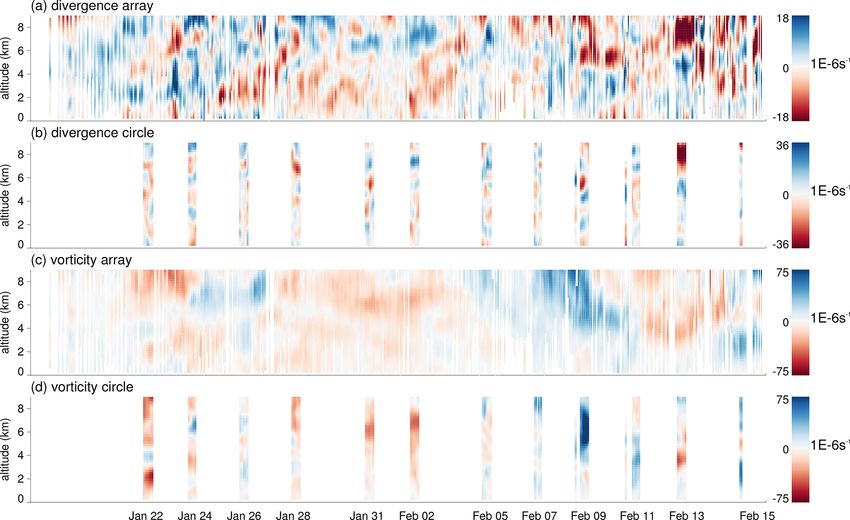
362                                                    C. C. Stephan and A. Mariaccia: Gravity waves and mesoscale motion

the analysis to areas with little distortion. For the blue poly-    of the selected time–wave number window. The initial alti-
gon in Fig. 1b, for instance, L/R = 1.3. The output of 3D-          tude interval [h0s , h0e ] is [0, 18] km. The degree of polariza-
Var contains the 3D fields of divergence and vorticity within       tion d is next computed for the initial window and all pos-
the polygon bounds. We average them horizontally to com-            sible combinations of shorter windows contained in it. The
pute vertical profiles of divergence and vorticity.                 window defined by [ts , te ], [hs , he ], where ts0 ≤ ts < te ≤ te0
                                                                    and h0s ≤ hs < he ≤ h0e , with the greatest total number of data
2.3   Hodograph analysis                                            points and a polarization d ≥ 0.8 is saved for subsequent
                                                                    analysis. If no window inside [ts0 , te0 ], [h0s , h0e ] with d ≥ 0.8
The hodographs of the horizontal wind perturbations asso-           can be found, then the peak is discarded. Otherwise  and 2
ciated with low-frequency gravity waves describe ellipses           are computed using the Stokes parameters.
whose properties can be determined using the Stokes param-             The angle 2 of the major axis of the ellipse counter-
eters, as in Eckermann and Vincent (1989). Properties that          clockwise from the eastward direction is the direction of
follow immediately are the ratio of the minor to the major          wave propagation, but with an ambiguity of 180◦ . To resolve
axis, ; the orientation of the major axis relative to the zonal    this ambiguity, we also compute this angle as in Evan and
direction, 2; and the degree of polarization of the ellipse, d.     Alexander (2008):
Large d indicates that a sounding contains coherent waves                                    0
                                                                                                !
                                                                                 −1   u0 T+90
rather than noise. Therefore, we iteratively search for time–       2T+90
                                                                        0  = tan                   ,                                  (1)
                                                                                             0
                                                                                      v 0 T+90
altitude windows in the radiosonde measurements that give
large values of d, as described in the following.                             0 is the value of the temperature perturbation after
                                                                    where T+90
   We analyze data from each platform separately, with one
                                                                    shifting the phase by +90◦ using a Hilbert transform. Finally,
exception: over the studied period, the MS-Merian launched
                                                                    the ratio  of the minor to the major axis is related to the
fewer radiosondes (118) than the others ships (Meteor: 203;
                                                                    intrinsic frequency  of the gravity wave as
RH-Brown: 169), which was partly due to her proximity to
the Atalante (139 radiosondes). Thus, to achieve continu-                f     kh mVz
                                                                    =     − 2              ,                                        (2)
ous data coverage, we include selected soundings collected                [m + 1/(4Hs2 )]
by the MS-Merian with those of the Atalante; specifically,
                                                                    where f is the Coriolis parameter, Hs the density scale
soundings of the MS-Merian that were taken within 100 km
                                                                    height, kh the magnitude of the horizontal wave number vec-
of the Atalante are added to the Atalante’s data set. This
                                                                    tor, and Vz = (dV /dz) the mean shear of the horizontal wind
choice is reasonable as the drift of a sonde can be on the order
                                                                    in the direction perpendicular to 2. To compute Vz , we first
of 100 km. From now on, we will refer to this merged data set
                                                                    average V over [hs , he ] and [ts , te ].
as the combined data set. The BCO is the only spatially fixed
                                                                       The dispersion relation for inertia–gravity waves (e.g.,
platform. They launched 182 sondes, whose horizontal wind
                                                                    Hankinson et al., 2014) is
measurements from 21 January at 02:00 UTC to 17 February
at 12:00 UTC are shown in Fig. 2a and b.                                               N 2 kh2             2f kh mV z
                                                                    2 = f 2 +                      −                ,             (3)
   Missing values in each data set are filled by interpolat-                     m2 + 1/     4Hs2        m + 1/ 4Hs2
                                                                                                          2
ing in time to a 1-hourly resolution. A Lanczos filter is ap-
                                                                    where N is the Brunt–Väisälä frequency. Combining Eq. (2)
plied to horizontal winds and temperature profiles to retain
                                                                    with Eq. (3) gives
vertical wavelengths of 500 m < λz < 10 km and periods of
3 h < τ < 53 h, where 53 h corresponds to the inertial period       2  2 − a 2 − 2f  1 − a 2 + f 2 1 − a 2 = 0,       (4)
at the BCO. Figure 2c and d show the resulting horizon-
tal wind perturbations for the BCO. Coherent structures are         where a 2 = Vz2 /(N 2 [1 + (4m2 Hs2 )−1 ]). Solving for f , this
clearly visible in both wind components. Oftentimes they ex-        results in
hibit a downward propagation with time, which is character-                          h                                 i1/2
                                                                                   2 ± 2 1 − a2 2 − 2 − a2 1 − a2

istic of upward-propagating gravity waves.                                 1 − a
   At each time we compute the quadrature spectrum be-                 =                                                      . (5)
                                                                    f                           2 − a2
tween the zonal and meridional wind perturbations, u0 (z)
                                                                    After determining , kh follows from the rearranged disper-
and v 0 (z). Then we search the resulting spectrum, which is a
                                                                    sion relation (3):
function of time and vertical wave number m, for local max-
ima in m that persist in time for at least 10 h. The vertical                      f mVz
profiles of u0 (z) and v 0 (z) are then filtered to include only    kh = kdisp =                                                     (6)
                                                                                    N2
the peak vertical wave number and the adjacent wave num-                                                        1/2
                                                                              1 f 2 m2 2  2
                                                                                                         1
bers. A first guess for the associated time window, [ts0 , te0 ],         ±           Vz +  − f 2
                                                                                                     m 2
                                                                                                         +            ,
is obtained from the positions of the adjacent minima. At                     N N2                         4Hs2
this point, the vertical wavelength assigned to the event is        where by definition kh is positive in the direction of wave
determined from the power-weighted mean wave number                 propagation.

Weather Clim. Dynam., 2, 359–372, 2021                                                   https://doi.org/10.5194/wcd-2-359-2021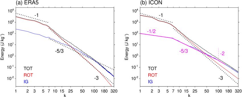
C. C. Stephan and A. Mariaccia: Gravity waves and mesoscale motion                                                             363

Figure 2. (a) Zonal and (b) meridional wind measured by ascending and descending soundings at the BCO. (c) Zonal and (d) meridional
wind perturbations after filtering the raw measurements to 500 m < λz < 10 km and 3 h < τ < 53 h.

     To obtain the ground-based frequency ω, we compute             For this reason we compute ω with the alternative method
at each altitude the quadrature spectrum between u0 (t) and         described above.
v 0 (t), QS(t, ν), using the S transformation (Stockwell et al.,
1996):                                                              2.4   Normal-mode decomposition of numerical data

QS(z; t, ν) = = STu (t, ν) · STv∗ (t, ν)

                                               z
                                                   ,        (7)     We derive global wave spectra as well as vertical profiles of
                                                                    regionally averaged divergence and vorticity from the ERA5
where STu (t, ν) is the S transformation in the time dimen-         reanalysis and a numerical simulation. For both data sets we
sion of u0 (t) at a given z, and ν denotes frequency. Then, ω       analyze 3-hourly horizontal winds between 20 January–29
corresponds to the peak in QS(z; t, ν) after integrating over       February 2020, matching the EUREC4 A period. The hodo-
[hs , he ] and [ts , te ].                                          graph analysis is not applied to the numerical data, because
   In principle we could estimate ω from the background             we found the vertical resolution to be too coarse.
wind in the direction of wave propagation, Uh , using ω =              ERA5 is produced and made publicly available by the
+kh Uh . However, due to the strong wind shear (see Fig. 2a        European Centre for Medium Range Weather Forecasts
and b), these results would be highly sensitive to the altitude     (ECMWF). The original data with a horizontal resolution of
range selected to compute Uh . As the Doppler shift equation        ∼ 30 km are stored on 137 hybrid sigma/pressure levels from
assumes Uh (z) = const, it is not clear if Uh is best approxi-      the surface up to an altitude of 80 km (0.01 hPa).
mated as an average across an altitude range or the wind at            The numerical simulation run at 2.5 km horizontal resolu-
a particular level. Moreover, as Uh is the projection of the        tion is performed with the ICON model (Zängl et al., 2015).
horizontal wind along the wave propagation direction, an ad-        It was initialized at 00:00 UTC on 20 January 2020 from an
ditional uncertainty is introduced by the uncertainty in 2.         operational analysis of the atmospheric state produced by the

https://doi.org/10.5194/wcd-2-359-2021                                               Weather Clim. Dynam., 2, 359–372, 2021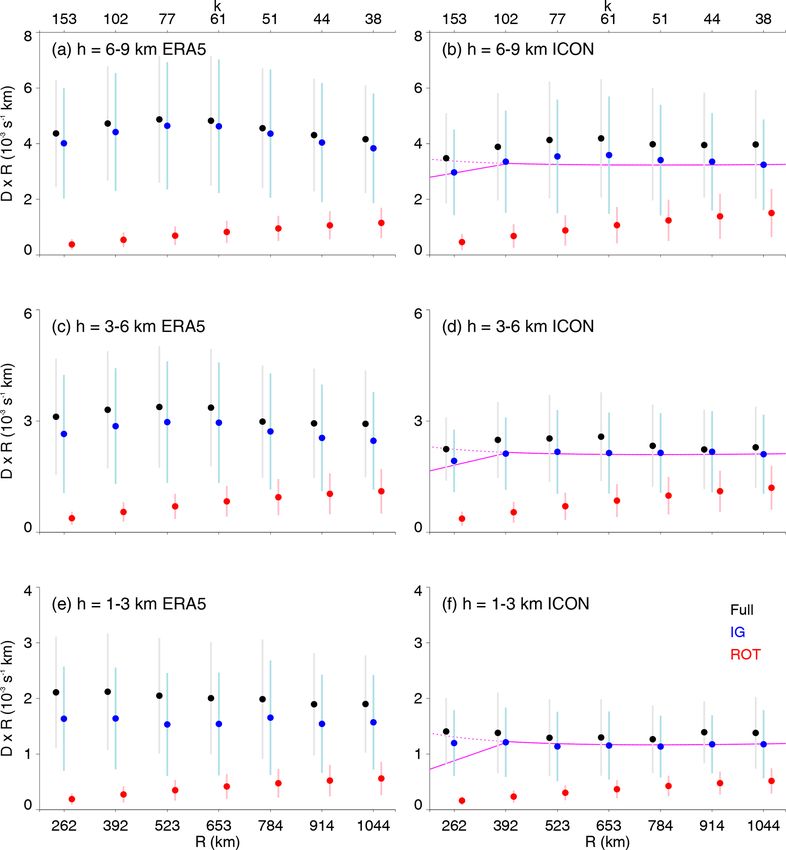
364                                                  C. C. Stephan and A. Mariaccia: Gravity waves and mesoscale motion

ECMWF and forced at the lower boundary with 7 d running-          possess only 3.8 % (ERA5) and 3.1 % (ICON) of the variance
mean sea surface temperatures, which are also taken from          contained in the ROT modes of Fig. 4c and d. Figure 4 also
an ECMWF analysis. Ninety vertical levels extend from the         shows strong variability at short scales in divergence and at
surface up to 75 km with a Klemp-type implicit Rayleigh           long scales in vorticity, with similar magnitudes to those ob-
damping (Klemp et al., 2008) of vertical winds starting at        served. Notably, 3D-Var, which ingests a 3 h running mean
44 km. The simulation is freely evolving and integrated until     of measurements, and MODES, which is independently ap-
00:00 UTC on 1 March 2020.                                        plied at single time steps, yield divergence as well as vor-
   We re-grid the data from both ERA5 and ICON to a reg-          ticity anomalies that exhibit temporal persistence with verti-
ular n256 Gaussian grid with 1024 × 512 points in longitude       cally coherent structures. From the comparison between ob-
and latitude, respectively, corresponding to a resolution of      servations and numerical data we conclude that by far the
39 km at the Equator. In the vertical we interpolate to 68 hy-    largest fraction of divergence variability inside the sounding
brid sigma/pressure levels between the surface and 10 hPa         network is due to IG waves.
(∼ 31 km).                                                           Because the EUREC4 A sounding network sampled areas
   The data at each time step are then subjected to a normal-     of different sizes, we can for the first time address how ob-
mode function decomposition, using the freely available           served magnitudes of area-averaged divergence variability
software package MODES, a detailed description of which           change with area. Figure 5 shows scatterplots of divergence
is given in Žagar et al. (2015). The modal decomposi-             amplitudes multiplied by the corresponding area-equivalent
tion projects the three-dimensional fields of geopotential        radius versus the equivalent radius for three different tropo-
height and horizontal wind onto an orthogonal set of ba-          spheric layers. We here define divergence amplitude as the
sis functions. These functions are solutions to the Rossby        difference between the maximum and minimum value found
and inertia–gravity wave (IG) dispersion relationships, re-       in a layer. The running means (thick blue dots) follow lines
spectively (Kasahara, 1976). Since the former are vorticity-      that are approximately horizontal, albeit with a slight upward
dominated, we label them as ROT. The orthogonality of the         slope at h = 6–9 km. Thus, divergence amplitudes at equiva-
basis functions allows filtering out specific wave modes, in-     lent radii of 100–300 km scale approximately inversely with
cluding the option of a subsequent inversion back to physical     radius.
space. This allows us to derive the local wind fields inside         ERA5 and ICON also show such an inverse scaling of di-
the EUREC4 A domain, as well as corresponding divergence          vergence amplitudes (Fig. 6). As expected from the predom-
and vorticity fields, associated with specific modes.             inant IG contribution to divergence, this scaling is due to the
                                                                  scaling of the IG-driven divergence field. While the lower
                                                                  bound in R is limited by our choice of normal-mode expan-
3     Results                                                     sion parameters, we can compute divergence for areas that
                                                                  exceed the sizes sampled during EUREC4 A. Figure 6 shows
3.1    Effects of the global wave spectrum on mesoscale           that the approximate R −1 scaling of divergence amplitudes
       divergence                                                 remains valid across the entire mesoscale, up to at least the
                                                                  synoptic scale of about 1000 km (zonal wave number 38).
Figure 3a and b show how vertical profiles of area-averaged       ERA5 and ICON produce qualitatively similar results, but
divergence vary in time. The strong vertical variability in the   we notice in Fig. 6 that ERA5 has slightly larger divergence
profiles derived from the array of all soundings and the cir-     amplitudes than ICON. To shed light on this difference and,
cle, respectively, is consistent with previous observations by    more importantly, to find an explanation for the scaling with
Bony and Stevens (2019) and Stephan et al. (2020a). Vortic-       radius, Fig. 7 examines the global energy spectra in ERA5
ity varies on longer scales in time–altitude space (Fig. 3c and   and ICON and their decomposition into IG and ROT modes.
d). For ERA5 and ICON we display the corresponding di-               In both data sets the total energy follows a k −1 power
vergence and vorticity profiles associated with IG and ROT        law at synoptic scales that transitions to a steeper slope at
modes, respectively (Fig. 4). These profiles are computed         k ≈ 8. For k > 8 the ROT spectrum in ERA5 scales as k −3 ,
for the same geographical region and an equivalent radius         and the IG spectrum follows on average a k −5/3 slope but
of ∼ 260 km. This radius corresponds to the smallest radius       with substantial deviations from a constant slope. Towards
that allows us to compute a centered area average, i.e., us-      the largest k there is a further steepening in ERA5, which
ing odd numbers of grid points in each direction on the n256      was also reported for ERA-Interim and points to a lack of
Gaussian grid, while at the same time exceeding the trun-         energy at small scales in the reanalysis (Žagar et al., 2015).
cation scales applied in the normal-mode decomposition in         The spectral behavior in ICON is similar to ERA5, but the
both horizontal directions (truncation meridional wave num-       slopes for different regimes are more sharply defined. The
ber n = 200; zonal wave number k = 320). Divergence as-           IG curve follows a k −1/2 slope for k < 8 and then k −5/3
sociated with ROT modes is negligible; ROT modes possess          up to k ≈ 100. At k > 100, there is a slight steepening in
only 2.4 % (ERA5) and 3.3 % (ICON) of the variance con-           ICON as well, such that the slope between k ≈ 100–150 is
tained in the IG modes of Fig. 4a and b. Similarly, IG modes      k −2 . The smallest scale shown in Fig. 6 is k = 153. The three

Weather Clim. Dynam., 2, 359–372, 2021                                               https://doi.org/10.5194/wcd-2-359-2021
C. C. Stephan and A. Mariaccia: Gravity waves and mesoscale motion 365 Figure 3. (a, b) Divergence and (c, d) vorticity anomalies derived from 3D-Var applied to (a, c) the sounding network and (b, d) the HALO circles. Figure 4. (a, b) Divergence and (c, d) vorticity anomalies associated with (a, b) IG and (c, d) ROT modes in (a, c) ERA5 and (b, d) ICON for an equivalent radius of 262 km. The area is centered on ∼ 12◦ N, −57◦ E, matching the approximate location of the EUREC4 A sounding network (compare Fig. 1b). https://doi.org/10.5194/wcd-2-359-2021 Weather Clim. Dynam., 2, 359–372, 2021
366                                                      C. C. Stephan and A. Mariaccia: Gravity waves and mesoscale motion

                                                                       As we will demonstrate in Sect. 3.2, the IG waves inside the
                                                                       EUREC4 A domain were mainly propagating zonally, so that
                                                                       we can assume divergence to scale as Div ∼ kAx (k). Near-
                                                                       zonal propagation is also expected, because IG waves can be-
                                                                       come equatorially trapped (Wheeler and Kiladis, 1999), and
                                                                       it is these equatorially trapped east- or westward-propagating
                                                                       modes that we identify with the normal-mode decomposi-
                                                                       tion. How Ax (k) depends on k is contained in the identified
                                                                       spectral slopes of IG modes in Fig. 7b: Ax scales as k −1/4 for
                                                                       k < 8, as k −5/6 for k = 8–100, and as k −1 for k = 100–150.
                                                                       To derive the relationship between these spectral slopes and
                                                                       the divergence amplitudes, we follow the ansatz that each av-
                                                                       eraging scale R ∗ = 2π/k ∗ feels the divergence on all scales
                                                                       R > R ∗ , whereas divergence at scales R < R ∗ has little or no
                                                                       effect. Under this assumption, the scaling of divergence am-
                                                                       plitudes AD (k ∗ ) can be approximated by the sum over all k
                                                                       smaller or equal to k ∗ = 2π/R ∗ :
                                                                                     X∗
                                                                                     k=k                  X∗
                                                                                                          k=k
                                                                       AD (k ∗ ) ∼         k · Ax (k) ∼         k · k σ (k) ,      (10)
                                                                                     k=1                  k=1
                                                                       with σ (k) ∈ {−1/4, −5/6, −1}, as indicated above. Comput-
                                                                       ing this sum and multiplying by a constant to match the IG
                                                                       point at R = 1044 km in Fig. 6b, d, and f results in the solid
                                                                       magenta lines drawn in these panels. Evidently, at 3–6 and
                                                                       6–9 km altitude, the match is excellent. At 1–3 km Fig. 6f
                                                                       misses the decrease in divergence magnitude at small R. This
Figure 5. Divergence amplitude anomaly (defined as maximum mi-
nus minimum at (a) 6–9 km, (b) 3–6 km, and (c) 1–3 km altitude)
                                                                       might be due to an introduction of additional energy at short
multiplied by equivalent radius, as a function of equivalent radius.   horizontal scales by convection, which tends to have tops
Based on divergence from 3D-Var applied to the sounding network.       at 1–2 km during EUREC4 A. We did not perform any cal-
Thick (thin) blue dots show the running mean (±1 standard devia-       culation for ERA5, as ERA5 clearly lacks energy at small
tion), using R intervals of 25 km.                                     scales and the ICON simulation is more realistic in this re-
                                                                       gard. However, as noted above, even in ICON the slope of
                                                                       the IG spectrum steepens slightly at k = 100. Since it is not
prominent slopes of k −1/2 , k −5/3 , and k −2 are marked with         clear if the change in spectral slope from k −5/6 to k −2 at
magenta lines in Fig. 7b. Figure 8 shows the energy con-               k = 100 is physical, we repeat the calculation using a slope
tained in IG modes in ERA5 relative to ICON. For k < 100               of k −5/6 for all k ≥ 8. This results in the dashed magenta
the energy in ERA5 exceeds the energy in ICON, and vice                lines of Fig. 6b, d, and f. Now, for R < 392 km there is no
versa for k > 100. Most of the divergence variability consid-          longer a drop in amplitude, but amplitudes remain approxi-
ered here can be attributed to the more energetic large scale,         mately constant. This behavior better matches the observa-
i.e., k < 100, explaining the larger divergence amplitudes in          tions (Fig. 5). The validity of Eq. (10) is further discussed in
ERA5.                                                                  Sect. 4.
   As it turns out, the spectral slopes can be used to predict
the magenta lines in Fig. 6b; i.e., they can explain how di-           3.2   Effects of individual waves on mesoscale divergence
vergence magnitudes vary with equivalent radius. Consider
a gravity wave with wave vector (k, l, m), frequency ω, and            In the previous section we related the characteristics of the
phase φ. The associated wind perturbations can be expressed            global IG spectrum to the statistical properties of variability
as                                                                     in area-averaged mesoscale divergence. We can now explain
                                                                       divergence magnitudes in a statistical sense, but the longevity
(u, v, w) = (Ax , Ay , Az ) sin(kx + ly + mz − ωt + φ),         (8)    of structures identified in Figs. 3 and 4 suggests that individ-
                                                                       ual waves may dominate the local divergence field at many
where the amplitudes Ai are functions of the wave vector.              times. It is important to note that the result obtained in the
The associated horizontal divergence scales with k and l as            previous section does not require a saturated wave spectrum.
follows:                                                               Evidently, the local spatiotemporal predominance of one or
                                                                       a few waves would change the scaling law in the given pe-
Div ∼ (kAx + lAy ) cos(kx + ly + mz − ωt + φ).                  (9)    riod and region, but this is consistent with the relatively large

Weather Clim. Dynam., 2, 359–372, 2021                                                        https://doi.org/10.5194/wcd-2-359-2021
C. C. Stephan and A. Mariaccia: Gravity waves and mesoscale motion 367 Figure 6. Divergence amplitude anomaly (defined as maximum minus minimum at (a) 6–9 km, (b) 3–6 km, and (c) 1–3 km altitude) in (a, c, d) ERA5 and (b, d, f) ICON. The vertical lines mark ±1 standard deviation. The solid magenta lines in panels (b, d, f) are theoretical predictions based on the spectra shown in Fig. 7 (see the text for details). The dashed magenta line uses a spectral slope of k −5/3 instead of k −2 at k > 100. Figure 7. (a, b) Energy spectra as a function of zonal wave number from MODES applied to (a) ERA5 and (b) ICON. The (black) total energy spectrum is decomposed into (red) ROT modes and (blue) IG modes. Dashed black lines show spectral slopes of k −1 , k −5/3 , and k −3 ; magenta lines in panel (b) show k −1/2 , k −5/3 , and k −2 , where the transition between k −5/3 and k −2 is at k = 100 and marked by a thin vertical magenta line. https://doi.org/10.5194/wcd-2-359-2021 Weather Clim. Dynam., 2, 359–372, 2021
368                                                 C. C. Stephan and A. Mariaccia: Gravity waves and mesoscale motion

Figure 8. Fraction of the energy in IG modes in ERA5 relative
to ICON as a function of zonal wave number (ERA5 divided by
ICON).

standard deviations in Figs. 5 and 6. Therefore, we next in-
vestigate if the generic IG waves that appear to govern the
statistics of mesoscale divergence can directly modulate con-
vection through their individual impact on mesoscale vertical    Figure 9. GOES-16 images from 31 January 2020, on a regu-
motion.                                                          lar longitude–latitude grid. The top edge of the images measures
                                                                 1358 km, the bottom edge 1410 km, and the sides 889 km. Shown
   To study local wave characteristics, we use the iterative
                                                                 are brightness temperatures from the C13 channel. Green outlines
hodograph algorithm, which is designed specifically to detect    show the Caribbean Islands, and red triangles the locations of
nearly monochromatic waves in soundings (see Sect. 2.3).         HALO’s dropsondes.
The algorithm extracted 34 wave events with polarization
d ≥ 0.8 and with an average polarization of 0.84. All events
and extracted wave characteristics are listed in Table 1. Most
detected waves have vertical wavelengths of 1.2–4 km with a      by narrow stripes of bright clouds. One of the larger cloud
mean of 2.6 km and highly variable horizontal wavelengths        clusters seen in the images is located inside the HALO cir-
with a mean and standard deviation of O(450) km. Intrinsic       cle. The top and bottom height of this cloud are ∼ 2.3 and
periods range from 6–45 h with a mean of 21 h, and ground-       ∼ 1 km, respectively. In the cloud layer the mean zonal wind
based periods from 11–50 h with a mean of 28 h. The average      is −4.3 m s−1 and the mean meridional wind is −0.1 m s−1 .
propagation direction, computed with two different methods,      Thus, the motion of the cloud cluster across the circle (diam-
is eastward.                                                     eter of 200 km) matches the estimated advection of 100 km
   The identified wave characteristics do not show any ev-       in 6.5 h.
idence for systematic changes over the period of the cam-           The 31st of January is also the day when the wave algo-
paign. This is consistent with a generally broad but unsatu-     rithm detected the most distinct wave event. Three out of the
rated tropospheric IG background. If the wave background         four data sets from the surface-based stations contain a wave
were saturated, then it would be impossible to identify waves    signal with a high degree of polarization (0.86, 0.86, 0.87;
with a high degree of polarization. Instead, at most times, we   Table 1). Notably, the three detected waves agree broadly
are able to find predominant waves (Table 1).                    in terms of the estimated horizontal wavelengths (480, 340,
   A day on which gravity waves may have had an effect on        440 km), which match well the 400 km spacing of the re-
the cloud field is 31 January. Figure 9 shows hourly infrared    spective moist or dry regions in Fig. 9. In addition, the long
satellite images of the campaign region on this day. A smooth    ground-based periods (33, 27, 34 h) are consistent with the
modulation of the cloud field is clearly visible in the form     nearly stationary appearance of the cloud field in Fig. 9.
of alternating southwest-to-northeast-oriented bands of dry         The propagation direction indicated by the algorithm,
and cloudy areas. The crests of the cloudy areas are topped      however, is more due eastward (−14◦ , −28◦ , −11◦ ) than

Weather Clim. Dynam., 2, 359–372, 2021                                               https://doi.org/10.5194/wcd-2-359-2021
C. C. Stephan and A. Mariaccia: Gravity waves and mesoscale motion 369
Table 1. For all identified wave events, columns list the (1) time interval t1 –t2 as “start date/start hour–end date/end hour” with hour in UTC,
(2) data set S (R: RH-Brown; M: Meteor; B: BCO; C: combined), (3) altitude interval h1 –h2 used for the computation of Stokes parameters,
(4) degree of polarization d, (5) wave propagation direction 2 counterclockwise from the eastward direction computed with the Stokes
parameters, (6) wave propagation direction 2T90 obtained with Eq. (1), (7) vertical wavelength λz , (8) horizontal wavelength λh , (9) intrinsic
period τ ∗ , and (10) ground-based period τ obtained from the quadrature spectrum.
t1 –t2 S h1 –h2 d 2 2T90 λz λh τ∗ τ
day/hour m ◦ ◦ m km h h
January
14/01–14/11 R 6000–15710 0.84 15 3 3306 718 29 19
18/15–19/00 R 4000–15710 0.81 −44 −3 2198 521 30 15
20/21–21/07 R 6000–13710 0.80 17 −3 1585 274 24 11
21/15–22/07 B 5030–15810 0.86 25 −9 5365 1836 37 21
23/23–24/17 M 6000–11750 0.86 34 −20 1043 103 14 27
25/05–25/19 M 6000–17750 0.80 4 −1 5190 226 7 25
25/08–26/10 B 13020–17810 0.80 18 −23 1848 234 19 41
26/04–26/16 C 6000–17640 0.82 2 1 2502 668 33 19
27/02–27/17 B 1030–13810 0.86 −13 4 4847 430 12 41
27/10–27/19 C 4000–15640 0.81 32 −10 1937 159 12 33
27/21–28/11 M 4000–15750 0.85 −27 9 2845 1561 45 22
28/07–29/02 C 0–17640 0.81 −16 20 3553 126 6 26
29/20–30/05 B 5030–15810 0.86 −4 2 2861 1100 39 19
29/21–31/02 R 8000–17710 0.81 −4 4 2526 861 38 33
31/14–01/00 C 3000–8640 0.85 −25 −2 1749 175 14 50
30/16–31/05 C 10000–17640 0.82 16 0 1596 174 17 50
31/05–01/00 B 7030–13810 0.86 −14 −3 3192 477 22 33
31/14–31/23 M 4000–7750 0.86 −28 −1 2286 339 20 27
31/17–01/02 R 5000–9710 0.87 −11 4 3962 441 16 34
February
01/01–01/16 M 6000–13750 0.85 0 −0.63 1302 120 14 19
01/22–02/12 B 3030–13810 0.86 20 −15 1279 68 8 36
02/20–03/07 C 5000–11000 0.85 −27 10 1944 138 10 41
01/07–02/06 R 4000–13710 0.80 −24 −7 2987 536 24 31
05/03–05/15 C 4000–11000 0.85 −15 −5 993 179 24 39
05/11–05/20 R 1000–10710 0.86 −33 −3 815 64 12 44
05/14–06/11 B 4030–7000 0.86 22 7 1062 191 23 22
05/12–05/22 M 0–3750 0.86 −12 −4 2435 111 8 16
07/05–07/17 C 0–17640 0.80 −41 10 1882 80 7 18
07/18–08/08 R 0–11710 0.80 28 6 4264 565 21 29
08/08–09/03 B 903–15810 0.85 0 5 6964 1395 27 33
08/21–09/09 R 6000–15710 0.82 21 −4 2895 417 21 15
09/13–10/04 B 5030–11810 0.85 −30 −7 2776 638 29 29
11/09–11/21 M 6000–13750 0.85 −41 0 775 41 8 12
15/17–16/07 B 13030–17810 0.86 27 9 3179 711 28 31
Average 0.84 −3 0 2645 461 21 28
SD 0.02 23 9 1434 445 10 11
one would expect from the alignment of the cloud pattern. HALO dropsonde profiles collected on 31 January over the
It could be that vertical propagation and refraction of the course of multiple circle flights. Their locations are marked
wave are partly responsible for this difference, because the by red triangles in Fig. 9. We pre-select the altitude inter-
ships were located further to the south, where a patterning of val of 2–5 km in order to include the upper portion of the
clouds is not visible (not shown). To obtain an additional es- cloud layer while avoiding noise near the surface. Since the
timate of wave parameters that allows for a more direct com- entire duration of the flight is less than 8 h, we compute wind
parison with Fig. 9, we apply a hodograph analysis to the 66 perturbations by removing the average of all profiles instead
https://doi.org/10.5194/wcd-2-359-2021 Weather Clim. Dynam., 2, 359–372, 2021370 C. C. Stephan and A. Mariaccia: Gravity waves and mesoscale motion
of filtering in time. The resulting horizontal wavelength is ages. Thus, although seldom, direct wave imprints on con-
421 km with a propagation angle 2 = −43.1◦ , in agreement vection do occur. This suggests that the IG wave background
with Fig. 9. is indeed not saturated. However, the systematic modula-
The good match of the satellite image with wave proper- tion of vertical motion due to IG waves of different scales
ties found independently in data from four stations is a strong may be more relevant for convection. More research is re-
indication for a causal link. The 31st of January was the only quired to quantify the relative importance of the stochas-
day that showed a potential wave imprint on the cloud field tic wave forcing for shaping patterns of convection, com-
that was detectable by eye. Thus, we conclude that visible ef- pared to other well-known local influences, such as lower-
fects of individual waves on convection occur rather seldom, tropospheric stability (Medeiros and Stevens, 2011), relative
at least during boreal winter in the studied region. humidity (Slingo, 1987), and sea surface temperature (Qu
et al., 2015).
Future studies should repeat the measurements analyzed in
4 Conclusions this study for different regions, especially different latitudes,
as well as regions over land, to test the universal applicabil-
This study extended the analysis of recent novel mea- ity of the proposed relationship between energy spectra and
surements of mesoscale divergence variability (Bony and divergence amplitudes. If confirmed, then our results imply
Stevens, 2019) by diagnosing vertical profiles of mesoscale that all scales are relevant for mesoscale variability, which
divergence in the extensive sounding network of the 2020 has consequences for regional models that introduce an ar-
EUREC4 A field campaign. For the first time, we could mea- tificial truncation scale, and could be used to design better
sure how divergence magnitudes depend on the area over external forcing methods for regional models.
which averages are computed, which may be relevant to sub-
daily variability of cloudiness (Mauger and Norris, 2010;
Vogel et al., 2020; George et al., 2020). Observed diver- Code availability. MODES software can be obtained at https:
gence magnitudes during EUREC4 A scale approximately in- //modes.cen.uni-hamburg.de/download (last access: 25 October
versely with the area-equivalent radius, a result that is also 2020). ERA5 is produced and made publicly available by the Eu-
true for the ERA5 reanalysis and a 2.5 km global numeri- ropean Centre for Medium Range Weather Forecasts (ECMWF).
cal simulation. By applying a normal-mode decomposition
to the numerical data, we demonstrated that the major frac-
Data availability. The vertically gridded (Level 2) radiosounding
tion of mesoscale divergence variability is due to inertia–
data described by Stephan et al. (2021) in NetCDF format are avail-
gravity (IG) waves, confirming the hypothesis put forward able to the public at https://doi.org/10.25326/62 (Stephan et al.,
by Stephan et al. (2020a). 2020b). GOES-16 Advanced Baseline Imager data are provided by
Moreover, we derived an analytic relationship between the NASA’s Worldview application (https://worldview.earthdata.nasa.
wave number dependence of global IG energy spectra and gov, last access: 24 November 2020). Data from the numerical sim-
the scaling of divergence amplitudes with area. The essen- ulation are stored by the Excellence in Science of Weather and Cli-
tial ansatz for this Eq. (10) is that IG waves on all scales mate in Europe (ESiWACE) project at the German Climate Com-
larger than a considered area contribute to the divergence av- puting Center (DKRZ).
eraged over this area. The data presented in this study follow
Eq. (10) very closely. Yet the relationship is not trivial from
an intellectual point of view, as one might expect some can- Author contributions. CCS conceptualized the study and prepared
celation of the local divergence induced by some IG waves the manuscript. AM carried out the hodograph analysis and pro-
with the local convergence associated with other IG waves. vided Fig. 2.
Either this cancelation has no effect on the overall scaling of
divergence amplitudes (note that Eq. 10 only predicts their
Competing interests. The authors declare that they have no conflict
scaling with area, not their absolute magnitude) or the cance-
of interest.
lation is negligible. The second possibility is more likely to
be true if the tropospheric IG wave background is not satu-
rated but locally composed of few waves. Persistent features Acknowledgements. Claudia Christine Stephan was supported by
in filtered-wind and divergence profiles suggest that the latter the Minerva Fast Track Programme of the Max Planck Society.
possibility may apply. She would like to thank David Raymond for his help with the
To gain more information about the properties of local 3D-Var software, which is openly available for download at http:
waves, we extracted nearly monochromatic wave events from //kestrel.nmt.edu/~raymond/software/candis/candis.html (last ac-
soundings by means of an iterative hodograph analysis. For cess: 21 October 2019). She is also grateful to Nedjeljka Žagar for
most days, clear IG signals could be found, and on one day her advice on using the MODES software.
the identified wave likely had a direct effect on the organi-
zation of clouds, as evidenced by comparison to satellite im-
Weather Clim. Dynam., 2, 359–372, 2021 https://doi.org/10.5194/wcd-2-359-2021C. C. Stephan and A. Mariaccia: Gravity waves and mesoscale motion 371
Financial support. This research has been supported by the Max- Kasahara, A.: Normal modes of ultralong waves in the atmosphere,
Planck-Gesellschaft. Mon. Weather Rev., 104, 669–690, 1976.
Klemp, J. B., Dudhia, J., and Hassiotis, A. D.: An upper gravity-
wave absorbing layer for NWP applications, Mon. Weather Rev.,
Review statement. This paper was edited by Pedram Hassanzadeh 136, 3987–4004, https://doi.org/10.1175/2008MWR2596.1,
and reviewed by two anonymous referees. 2008.
Lane, T. P. and Zhang, F.: Coupling between gravity waves and trop-
ical convection at mesoscales, J. Atmos. Sci., 68, 2582–2598,
https://doi.org/10.1175/2011JAS3577.1, 2011.
López Carrillo, C. and Raymond, D. J.: Retrieval of three-
References dimensional wind fields from Doppler radar data using an ef-
ficient two-step approach, Atmos. Meas. Tech., 4, 2717–2733,
Albrecht, B. A., Betts, A. K., Schubert, W. H., and Cox, https://doi.org/10.5194/amt-4-2717-2011, 2011.
S. K.: Model of the thermodynamic structure of the trade-wind Mauger, G. S. and Norris, J. R.: Assessing the impact of meteoro-
boundary layer: Part I. Theoretical formulation and sensitivity logical history on subtropical cloud fraction, J. Clim., 23, 2926–
tests, J. Atmos. Sci., 36, 73–89, https://doi.org/10.1175/1520- 2940, https://doi.org/10.1175/2010JCLI3272.1, 2010.
0469(1979)0362.0.CO;2, 1979. May, P. T., Mather, J. H., Vaughan, G., Jakob, C., McFarquhar,
Albrecht, B. A., Jensen, M. P., and Syrett, W. J.: Marine bound- G. M., Bower, K. N., and Mace, G. G.: The Tropical Warm
ary layer structure and fractional cloudiness, J. Geophys. Res.- Pool-International Cloud Experiment, B. Am. Meteorol. Soc.,
Atmos., 100, 14209–14222, https://doi.org/10.1029/95JD00827, 89, 629–645, https://doi.org/10.1175/BAMS-89-5-629, 2008.
1995. Medeiros, B. and Stevens, B.: Revealing differences in GCM
Boer, G. J. and Shepherd, T. G.: Large-scale two-dimensional tur- representations of low clouds, Clim. Dyn., 36, 385–399,
bulence in the atmosphere, J. Atmos. Sci., 40, 164–184, 1983. https://doi.org/10.1007/s00382-009-0694-5, 2011.
Bony, S. and Stevens, B.: Measuring area-averaged verti- Nastrom, G. D. and Gage, K. S.: A climatology of aircraft
cal motions with dropsondes, J. Atmos. Sci., 76, 767–783, wavenumber spectra observed by commercial aircraft, J. Atmos.
https://doi.org/10.1175/JAS-D-18-0141.1, 2019. Sci., 42, 950–960, 1985.
Bony, S., Stevens, B., Ament, F., Bigorre, S., Chazette, P., Crewell, NOAA: NOAA GOES-R series Advanced Baseline Imager
S., Delanoë, J., Emanuel, K., Farrell, D., Flamant, C., Gross, (ABI) Level 2 cloud top height (ACHA). GOES-R al-
S., Hirsch, L., Karstensen, J., Mayer, B., Nuijens, L., Rup- gorithm working group, and GOES-R series program of-
pert, J. H., Sandu, I., Siebesma, P., Speich, S., Szczap, F., fice, NOAA national centers for environmental Information,
Totems, J., Vogel, R., Wendisch, M., and Wirth, M.: EUREC4A: https://doi.org/10.7289/V5HX19ZQ, 2018.
A field campaign to elucidate the couplings between clouds, Norris, J. R.: Low cloud type over the ocean from sur-
convection and circulation, Surv. Geophys., 38, 1529–1568, face observations. Part I: Relationship to surface meteorol-
https://doi.org/10.1007/s10712-017-9428-0, 2017. ogy and the vertical distribution of temperature and mois-
Eckermann, S. D. and Vincent, R. A.: Falling sphere observa- ture, J. Clim., 11, 369–382, https://doi.org/10.1175/1520-
tions of anisotropic gravity wave motions in the upper strato- 0442(1998)0112.0.CO;2, 1998.
sphere over Australia, Pure Appl. Geophys., 130, 509–532, Nuijens, L., Medeiros, B., Sandu, I., and Ahlgrimm, M.: The be-
https://doi.org/10.1007/BF00874472, 1989. havior of trade-wind cloudiness in observations and models: The
Evan, S. and Alexander, M. J.: Intermediate-scale trop- major cloud components and their variability, J. Adv. Mod. Earth
ical inertia gravity waves observed during the TWP- Sys., 7, 600–616, https://doi.org/10.1002/2014MS000390, 2015.
ICE campaign, J. Geophys. Res., 113, D14101, Qu, X., Hall, A., Klein, S. A., and DeAngelis, A. M.: Posi-
https://doi.org/10.1029/2007JD009289, 2008. tive tropical marine low-cloud cover feedback inferred from
George, G., Stevens, B., Bony, S., Klingebiel, M., and Vogel, R.: cloud-controlling factors, Geophys. Res. Lett., 42, 7767–7775,
Observed impact of meso-scale vertical motion on cloudiness, J. https://doi.org/10.1002/2015GL065627, 2015.
Atmos. Sci., under review, 2020. Schmit, T. J., Griffith, P., Gunshor, M. M., Daniels, J. M., Good-
Hankinson, M. C. N., Reeder, M. J., and Lane, T. P.: Gravity man, S. J., and Lebair, W. J.: A closer look at the ABI
waves generated by convection during TWP-ICE: I. Inertia- on the GOES-R series, B. Am. Meteorol. Soc. 98, 681–698,
gravity waves, J. Geophys. Res.-Atmos., 119, 5269–5282, https://doi.org/10.1175/BAMS-D-15-00230.1, 2017.
https://doi.org/10.1002/2013JD020724, 2014. Shige, S. and Satomura, T.: Westward generation of eastward-
Hersbach, H., Bell, B., Berrisford, P., Hirahara, S., Horányi, A., moving tropical convective bands in TOGA COARE, J.
Muñoz-Sabater, J., Nicolas, J., Peubey, C., Radu, R., Schepers, Atmos. Sci., 58, 3724–3740, https://doi.org/10.1175/1520-
D., Simmons, A., Soci, C., Abdalla, S., Abellan, X., Balsamo, 0469(2001)0582.0.CO%3B2, 2001.
G., Bechtold, P., Biavati, G., Bidlot, J., Bonavita, M., De Chiara, Slingo, J. M.: The development and verification of a cloud predic-
G., Dahlgren, P., Dee, D., Diamantakis, M., Dragani, R., Flem- tion scheme for the ECMWF model, Q. J. Roy. Meteor. Soc.,
ming, J., Forbes, R., Fuentes, M., Geer, A., Haimberger, L., 113, 899–927, https://doi.org/10.1002/qj.49711347710, 1987.
Healy, S., Hogan, R. J., Hólm, E., Janisková, M., Keeley, S., Sobel, A. H. and Bretherton, C. S.: Modeling trop-
Laloyaux, P., Lopez, P., Lupu, C., Radnoti, G., de Rosnay, P., ical precipitation in a single column, J. Clim.,
Rozum, I., Vamborg, F., Villaume, S., and Thépaut, J.-N.: The 13, 4378–4392, https://doi.org/10.1175/1520-
ERA5 global reanalysis, Q. J. Roy. Meteor. Soc., 146, 1999– 0442(2000)0132.0.CO;2, 2000.
2049, https://doi.org/10.1002/qj.3803, 2020.
https://doi.org/10.5194/wcd-2-359-2021 Weather Clim. Dynam., 2, 359–372, 2021372 C. C. Stephan and A. Mariaccia: Gravity waves and mesoscale motion Stechmann, S. N. and Majda, A. J.: Gravity waves in shear and im- O., Luneau, C., Makuch, P., Malinowski, S., Manta, G., Mari- plications for organized convection, J. Atmos. Sci., 66, 2579– nou, E., Marsden, N., Masson, S., Maury, N., Mayer, B., Mayers- 2599, https://doi.org/10.1175/2009JAS2976.1, 2009. Als, M., Mazel, C., McGeary, W., McWilliams, J. C., Mech, Stephan, C. C., Lane, T. P., and Jakob, C.: Gravity wave M., Mehlmann, M., Meroni, A. N., Mieslinger, T., Minikin, A., influences on mesoscale divergence: An observational Minnett, P., Möller, G., Morfa Avalos, Y., Muller, C., Musat, I., case study, Geophys. Res. Lett., 47, e2019GL086539, Napoli, A., Neuberger, A., Noisel, C., Noone, D., Nordsiek, F., https://doi.org/10.1029/2019GL086539, 2020a. Nowak, J. L., Oswald, L., Parker, D. J., Peck, C., Person, R., Stephan, C., Schnitt, S., Schulz, H., and Bellenger, H.: Radiosonde Philippi, M., Plueddemann, A., Pöhlker, C., Pörtge, V., Pöschl, measurements from the EUREC4A field campaign, [data set], U., Pologne, L., Posyniak, M., Prange, M., Quiñones Meléndez, https://doi.org/10.25326/62, 2020b. E., Radtke, J., Ramage, K., Reimann, J., Renault, L., Reus, K., Stephan, C. C., Schnitt, S., Schulz, H., Bellenger, H., de Szoeke, Reyes, A., Ribbe, J., Ringel, M., Ritschel, M., Rocha, C. B., S. P., Acquistapace, C., Baier, K., Dauhut, T., Laxenaire, R., Rochetin, N., Röttenbacher, J., Rollo, C., Royer, H., Sadoulet, Morfa-Avalos, Y., Person, R., Quiñones Meléndez, E., Bagheri, P., Saffin, L., Sandiford, S., Sandu, I., Schäfer, M., Schemann, G., Böck, T., Daley, A., Güttler, J., Helfer, K. C., Los, S. V., Schirmacher, I., Schlenczek, O., Schmidt, J., Schröder, M., A., Neuberger, A., Röttenbacher, J., Raeke, A., Ringel, M., Schwarzenboeck, A., Sealy, A., Senff, C. J., Serikov, I., Shohan, Ritschel, M., Sadoulet, P., Schirmacher, I., Stolla, M. K., Wright, S., Siddle, E., Smirnov, A., Späth, F., Spooner, B., Stolla, M. E., Charpentier, B., Doerenbecher, A., Wilson, R., Jansen, F., K., Szkółka, W., de Szoeke, S. P., Tarot, S., Tetoni, E., Thomp- Kinne, S., Reverdin, G., Speich, S., Bony, S., and Stevens, B.: son, E., Thomson, J., Tomassini, L., Totems, J., Ubele, A. A., Ship- and island-based atmospheric soundings from the 2020 Villiger, L., von Arx, J., Wagner, T., Walther, A., Webber, B., EUREC4 A field campaign, Earth Syst. Sci. Data, 13, 491–514, Wendisch, M., Whitehall, S., Wiltshire, A., Wing, A. A., Wirth, https://doi.org/10.5194/essd-13-491-2021, 2021. M., Wiskandt, J., Wolf, K., Worbes, L., Wright, E., Wulfmeyer, Stevens, B., Bony, S., Farrell, D., Ament, F., Blyth, A., Fairall, V., Young, S., Zhang, C., Zhang, D., Ziemen, F., Zinner, T., and C., Karstensen, J., Quinn, P. K., Speich, S., Acquistapace, C., Zöger, M.: EUREC4A, Earth Syst. Sci. Data Discuss. [preprint], Aemisegger, F., Albright, A. L., Bellenger, H., Bodenschatz, https://doi.org/10.5194/essd-2021-18, in review, 2021. E., Caesar, K.-A., Chewitt-Lucas, R., de Boer, G., Delanoë, J., Stockwell, R. G., Mansinha, L., and Lowe, R. P.: Localization of Denby, L., Ewald, F., Fildier, B., Forde, M., George, G., Gross, the complex spectrum: the S transform, IEEE T. Signal Proces., S., Hagen, M., Hausold, A., Heywood, K. J., Hirsch, L., Jacob, 44, 998–1001, https://doi.org/10.1109/78.492555, 1996. M., Jansen, F., Kinne, S., Klocke, D., Kölling, T., Konow, H., van der Dussen, J. J., de Roode, S. R., and Siebesma, A. P.: How Lothon, M., Mohr, W., Naumann, A. K., Nuijens, L., Olivier, large-scale subsidence affects stratocumulus transitions, Atmos. L., Pincus, R., Pöhlker, M., Reverdin, G., Roberts, G., Schnitt, Chem. Phys., 16, 691–701, https://doi.org/10.5194/acp-16-691- S., Schulz, H., Siebesma, A. P., Stephan, C. C., Sullivan, P., 2016, 2016. Touzé-Peiffer, L., Vial, J., Vogel, R., Zuidema, P., Alexander, N., Vogel, R., Bony, S., and Stevens, B.: Estimating the shallow convec- Alves, L., Arixi, S., Asmath, H., Bagheri, G., Baier, K., Bai- tive mass flux from the subcloud-layer mass budget, J. Atmos. ley, A., Baranowski, D., Baron, A., Barrau, S., Barrett, P. A., Sci., 77, 1559–1574, https://doi.org/10.1175/JAS-D-19-0135.1, Batier, F., Behrendt, A., Bendinger, A., Beucher, F., Bigorre, S., 2020. Blades, E., Blossey, P., Bock, O., Böing, S., Bosser, P., Bourras, Žagar, N., Kasahara, A., Terasaki, K., Tribbia, J., and Tanaka, H.: D., Bouruet-Aubertot, P., Bower, K., Branellec, P., Branger, H., Normal-mode function representation of global 3-D data sets: Brennek, M., Brewer, A., Brilouet, P.-E., Brügmann, B., Buehler, open-access software for the atmospheric research community, S. A., Burke, E., Burton, R., Calmer, R., Canonici, J.-C., Carton, Geosci. Model Dev., 8, 1169–1195, https://doi.org/10.5194/gmd- X., Cato Jr., G., Charles, J. A., Chazette, P., Chen, Y., Chilinski, 8-1169-2015, 2015. M. T., Choularton, T., Chuang, P., Clarke, S., Coe, H., Cornet, Wheeler, M. and Kiladis, G. N.: Convectively Coupled C., Coutris, P., Couvreux, F., Crewell, S., Cronin, T., Cui, Z., Equatorial Waves: Analysis of Clouds and Temper- Cuypers, Y., Daley, A., Damerell, G. M., Dauhut, T., Deneke, H., ature in the Wavenumber–Frequency Domain, J. At- Desbios, J.-P., Dörner, S., Donner, S., Douet, V., Drushka, K., mos. Sci., 56, 374–399, https://doi.org/10.1175/1520- Dütsch, M., Ehrlich, A., Emanuel, K., Emmanouilidis, A., Eti- 0469(1999)0562.0.CO;2, 1999. enne, J.-C., Etienne-Leblanc, S., Faure, G., Feingold, G., Ferrero, Wood, R. and Hartmann, D. L.: Spatial variability of liq- L., Fix, A., Flamant, C., Flatau, P. J., Foltz, G. R., Forster, L., uid water path in marine low cloud: The importance of Furtuna, I., Gadian, A., Galewsky, J., Gallagher, M., Gallimore, mesoscale cellular convection, J. Clim., 19, 1748–1764, P., Gaston, C., Gentemann, C., Geyskens, N., Giez, A., Gollop, https://doi.org/10.1175/JCLI3702.1, 2006. J., Gouirand, I., Gourbeyre, C., de Graaf, D., de Groot, G. E., Zängl, G., Reinert, D., Ripodas, P., and Baldauf, M.: The Grosz, R., Güttler, J., Gutleben, M., Hall, K., Harris, G., Helfer, ICON (ICOsahedral Non-hydrostatic) modelling framework K. C., Henze, D., Herbert, C., Holanda, B., Ibanez-Landeta, A., of DWD and MPI-M: Description of the non-hydrostatic Intrieri, J., Iyer, S., Julien, F., Kalesse, H., Kazil, J., Kellman, A., dynamical core, Q. J. Roy. Meteor. Soc., 141, 563–579, Kidane, A. T., Kirchner, U., Klingebiel, M., Körner, M., Krem- https://doi.org/10.1002/qj.2378, 2015. per, L. A., Kretzschmar, J., Krüger, O., Kumala, W., Kurz, A., L’Hégaret, P., Labaste, M., Lachlan-Cope, T., Laing, A., Land- schützer, P., Lang, T., Lange, D., Lange, I., Laplace, C., Lavik, G., Laxenaire, R., Le Bihan, C., Leandro, M., Lefevre, N., Lena, M., Lenschow, D., Li, Q., Lloyd, G., Los, S., Losi, N., Lovell, Weather Clim. Dynam., 2, 359–372, 2021 https://doi.org/10.5194/wcd-2-359-2021
You can also read