Diffusion of colloidal rods in corrugated channels - Uni Augsburg : Physik
←
→
Page content transcription
If your browser does not render page correctly, please read the page content below

PHYSICAL REVIEW E 99, 020601(R) (2019)
 Rapid Communications

                                      Diffusion of colloidal rods in corrugated channels
     Xiang Yang,1 Qian Zhu,1 Chang Liu,1 Wei Wang,2 Yunyun Li,3 Fabio Marchesoni,3,4 Peter Hänggi,5,6 and H. P. Zhang1,7,*
             1
               School of Physics and Astronomy and Institute of Natural Sciences, Shanghai Jiao Tong University, Shanghai, China
                   2
                     School of Materials Science and Engineering, Harbin Institute of Technology (Shenzhen), Shenzhen, China
      3
        Center for Phononics and Thermal Energy Science, School of Physics Science and Engineering, Tongji University, Shanghai, China
                                     4
                                       Dipartimento di Fisica, Università di Camerino, I-62032 Camerino, Italy
                                       5
                                         Institut für Physik, Universität Augsburg, D-86135 Augsburg, Germany
                                6
                                  Nanosystems Initiative Munich, Schellingstrasse 4, D-80799 München, Germany
                                  7
                                    Collaborative Innovation Center of Advanced Microstructures, Nanjing, China

                                                 (Received 23 July 2018; published 21 February 2019)

                    In many natural and artificial devices diffusive transport takes place in confined geometries with corrugated
                 boundaries. Such boundaries cause both entropic and hydrodynamic effects, which have been studied only for
                 the case of spherical particles. Here we experimentally investigate the diffusion of particles of elongated shape
                 confined in a corrugated quasi-two-dimensional channel. The elongated shape causes complex excluded-volume
                 interactions between particles and channel walls which reduce the accessible configuration space and lead to
                 novel entropic free-energy effects. The extra rotational degree of freedom also gives rise to a complex diffusivity
                 matrix that depends on both the particle location and its orientation. We further show how to extend the standard
                 Fick-Jacobs theory to incorporate combined hydrodynamic and entropic effects, so as, for instance, to accurately
                 predict experimentally measured mean first passage times along the channel. Our approach can be used as a
                 generic method to describe translational diffusion of anisotropic particles in corrugated channels.

                 DOI: 10.1103/PhysRevE.99.020601

   Diffusive transport through microstructures such as occur-                equation must then be amended in terms of the experimentally
ring in porous media [1,2], micro- and nanofluidic channels                  measured particle diffusivity.
[3–7], and living tissues [8,9], is ubiquitous and attracts ever-                Previous studies on confined diffusion focused mostly on
growing attention from physicists [10,11], mathematicians                    spherical particles, for which only the translational d.o.f.’s
[12], engineers [1], and biologists [8,9,13]. A common feature               were considered. However, particles in practical applications
of these systems is confining boundaries of irregular shapes.                appear inherently more complex in exhibiting anisotropic
Spatial confinement can fundamentally change the equilib-                    shape and possessing additional degrees of freedom other
rium and dynamical properties of a system by both limiting                   than translational. For example, anisotropic particles, such as
the configuration space accessible to its diffusing components               colloids [24–28], artificial and biological filaments [29,30],
[10] and increasing the hydrodynamic drag [14] on them.                      DNA strands [31,32], and microswimmers [33,34], exhibit
   An archetypal model to study confinement effects consists                 complex coupling between rotation and translation, even in
of a spherical particle diffusing in a corrugated narrow                     the absence of geometric constraints. How can complex shape
channel, which mimics directed ionic channels [15], zeolites                 and additional d.o.f.’s such as rotation alter the current picture
[16], and nanopores [17]. In this context, Jacobs [18] and                   of confined diffusion? Here, we address this open question and
Zwanzig [19] proposed a theoretical formulation to account                   study how a colloidal rod diffuses in a quasi-two-dimensional
for the entropic effects stemming from constrained transverse                (2D) corrugated channel [35]. Our experiments reveal that the
diffusion. Focusing on the transport (channel) direction, they               interplay of a channel’s spatial modulation, a rod’s shape, and
assumed that the transverse degrees of freedom (d.o.f.’s)                    rotational dynamics causes substantial hydrodynamic and en-
equilibrate sufficiently fast and can, therefore, be eliminated              tropic effects. We succeed in extending the standard FJ theory
adiabatically by means of an approximate projection scheme.                  to incorporate both effects; the resulting theory accurately pre-
In first order, they derived a reduced diffusion equation in the             dicts the experimentally measured mean first-passage times
channel direction, known as the Fick-Jacobs (FJ) equation.                   (MFPTs) associated with rod translation along the channel.
Numerical investigations [11,20–23] demonstrated that the                        Experimental setup. Our channels were fabricated on a
FJ equation provides a useful tool to accurately estimate the                coverslip by means of a two-photon direct laser writing sys-
entropic effects for confined pointlike particles. However,                  tem, which solidifies polymers according to a preassigned
our recent experiments [5] evidentiated that hydrodynamic                    channel profile, f (x), with a submicron resolution [5]. As
effects for finite size particles cannot be disregarded if                   depicted in Fig. 1(a), the quasi-2D channel has a uniform
the channel and particle dimensions grow comparable. In                      height (denoted by H). In the central region, the periodically
order to incorporate such hydrodynamic corrections, the FJ                   curved lateral walls form cells of length L with inner bound-
                                                                             aries a distance y = ±h(x) away from the channel’s axis.
                                                                             The preassigned profile f (x) is given the form of a cosine,
 *
     hepeng_zhang@sjtu.edu.cn                                                which tapers off to a constant in correspondence with the cell

2470-0045/2019/99(2)/020601(5)                                       020601-1                                  ©2019 American Physical Society
XIANG YANG et al.                                                                                  PHYSICAL REVIEW E 99, 020601(R) (2019)

                                                                             length 2lX , which varies in the range 1.6–3.2 μm. Using a
                                                                             magnet, we dragged a rod into the channel through a narrow
                                                                             entrance, which creates insurmountable entropic barriers to
                                                                             prevent the rod from exiting the channel. The rod’s motion
                                                                             in such quasi-2D channel was recorded through a microscope
                                                                             at 30 frames per second for up to 20 h [5]. We tracked
                                                                             rod trajectories in the imaging plane and extracted its center
                                                                             coordinates, (x, y), and tilting angle, θ , by standard particle-
                                                                             tracking algorithms. We detected no sizable rod dynamics in
                                                                             the out-of-plane direction (see Movie S1.mp4 in the Supple-
                                                                             mental Material [36]).
                                                                                 A typical rod trajectory is displayed in Fig. 1(b). The
                                                                             channel boundaries limit the space accessible to the rod and
                                                                             such a limiting effect depends on the rod’s orientation: the
                                                                             rod gets closer to the boundary if it is aligned tangent to
                                                                             the walls. To quantify this orientation-dependent effect, we
                                                                             distributed the recorded rod’s center coordinates, (x, y), for a
                                                                             given orientation, θ , into small bins (0.26 μm × 0.2 μm) and
                                                                             counted how many times the rod’s center was to be found in
                                                                             each bin. The resulting rod center distributions for three values
                                                                             of θ are plotted in Fig. 2(a). Nearly uniform distributions
                                                                             demonstrate that the rod diffuses in a flat energy landscape,
                                                                             whereas sharp drops of the distributions near the boundaries
                                                                             mark the edge of the accessible space, consistently with y =
                                                                             g± (x, θ ) computed from the excluded-volume considerations
                                                                             [see Fig. 2(a)]. The channel boundaries also affect the rod’s
                                                                             orientation. For instance, when the rod is relatively long,
                                                                             namely, for hn < lX , then it tends to orient itself parallel to
                                                                             the channel direction inside the neck region, as illustrated in
                                                                             the middle panel of Fig. 2(a).
                                                                                 Fick-Jacobs free energy. The rod diffusion can be de-
    FIG. 1. (a) Electron scanning image of a thin channel (H =               scribed as a random walk in the configuration space (x, y, θ ).
1.0 μm, α = 7/8). Narrow openings at the two ends are marked                 The dashed curves y = g± (x, θ ) in Fig. 2(a) illustrate how
by red asterisks. The inset illustrates a section of the channel with        the walls limit the channel’s space accessible to the rod’s
laser-scanning contour, f (x), wall inner boundary, h(x), and upper          center for three different θ values. From these curves one
effective boundary, g+ (x, θ ), delimiting the region accessible to the      can construct a surface in the configuration space, as shown
center of a rod with a given tilting angle, θ . Rod’s length and width       in Fig. 2(b), and model the motion of the confined rod as
and wall thickness are denoted, respectively, by 2lX , 2lY , and dt . The    that of a pointlike particle diffusing inside the reconstructed
coordinates x, y, z and X, Y refer, respectively, to the laboratory and      three-dimensional (3D) channel enclosed by that surface. For
body frames. (b) Sample of time discretized trajectory (dotted line)         a rod with length of about 1 μm, the relaxation times of
for a rod with lX = 1.5 μm in a tall channel (H = 2.0 μm, α = 1);            θ and y are short enough for the FJ approach to closely
the rod’s orientation at different times is also reported according to       reproduce the long-time diffusion in the reconstructed 3D
the depicted color code.                                                     channel (see Supplemental Material Sec. II B [36]). To that
                                                                             end, we integrate the probability density ρ(x, y, θ , t ) to ob-
connecting ducts, or necks, that is,                                         tain p(x, t ) =     ρ(x, y, θ , t )dy dθ and the corresponding FJ
                                                                            equation governing its time evolution,
                                                                αL
             1
               ( f + fn ) + 21 ( fw − fn )cos 2πx
             2 w                              αL
                                                  , |x| <                     ∂ p(x, t )    ∂          ∂ p(x, t )            ∂        G(x)
   f (x) =         αL
                                                                   2
                                                                                         =      D(x)              + p(x, t )     − ln         .
             fn ,   2
                       |x| < 2 L.1
                                                                                 ∂t        ∂x             ∂x                 ∂x       G(0)
                                                                       (1)                                                                     (2)
                                                                                                   π/2
The minimum (maximum) half-width of f (x) is denoted by                      Here, G(x) =     1
                                                                                             2π    −π/2 [g+ (x, θ ) − g− (x, θ )]dθ represents the
 fn(w) , respectively, whereas (1 − α)L is the length of the neck.           area of the (y, θ ) cross section of the reconstructed 3D channel
Due to the lateral wall thickness dt = 0.8 μm [see inset of                  at a given point x. Three such cross sections are plotted in
Fig. 1(a)], f (x) and h(x) are separated by a distance dt /2,                Fig. 2(c). Restrictions in both the center coordinates, (x, y),
so that fn(w) = hn(w) + dt /2. We changed fn continuously for                and the tilting angle, θ , cause variation of G(x). The latter
fixed L = 12 μm and fw = 4.6 μm, while for the remaining                     effect is most pronounced in the neck regions, as illustrated
channel parameters we considered two typical geometries:                     by the blue cross section in Fig. 2(c). Consequently, the
tall channels (H = 2.0 μm, α = 1) and thin channels (H =                     variations of G(x) modulate the FJ free-energy profile along
1.0 μm, α = 7/8).                                                            the channel. The free-energy potentials plotted in Fig. 2(d),
    After fabrication, channels were immersed in water with                  − ln[G(x)/G(0)], exhibit barriers of about 1.8kB T for a rod
suspended iron-plated gold rods of width 2lY = 0.3 μm and                    with a half-length lX = 1.6 μm, which is 50% higher than that

                                                                       020601-2
DIFFUSION OF COLLOIDAL RODS IN CORRUGATED …                                                          PHYSICAL REVIEW E 99, 020601(R) (2019)

    FIG. 2. (a) Spatial distributions of the rod center for three tilting angles, θ = π6 , π2 , and − π6 . The channel’s inner boundaries, y = ±h(x), and
the tilt-dependent effective boundaries, y = g± (x, θ ), are marked by solid and dashed lines, respectively. (b) The configuration space accessible
to the confined rod is delimited by the surfaces y = g± (x, θ ). Five cross sections are shown in color; three of them, at x/L = 0, 0.22, and 0.46,
are displayed in (c). (d) Free-energy profile (in units of kB T ), − ln[G(x)/G(0)], for different rod lengths (see text). The black line represents
the case of a sphere of radius lX = 0.15 μm. Data in (a)–(d) were obtained in a tall channel (H = 2.0 μm, α = 1) with hn = 1.8 μm, while
the rod used in (a)–(c) had half-length lX = 1.6 μm.

of a sphere. This novel entropic effect is induced by particle                 Figure 3(a) displays the function Dave (x) for three different
shape and its strength increases with increasing rod length.                   rod lengths. While for the shortest rod (lX = 1.0 μm) Dave (x)
   Fick-Jacobs effective diffusivity. Apart from the entropic                  exhibits minor variability along the channel, for the longest
potential, the FJ approach introduces an effective longitudinal                rod (lX = 1.6 μm) Dave (x) is about 30% larger in the neck re-
diffusivity function, D(x) in Eq. (2). To estimate it, we first                gions than at the center of the channel cells. This surprising re-
determined the local diffusivity matrix DIJ (x, y, θ ) of a rod                sult can be explained by inspecting the corresponding angular
located at (x, y) with angle θ , where I and J represent any                   distributions in Fig. 3(b). While around the center of the chan-
pair of coordinates X , Y , or θ in the body frame. As shown                   nel cell the rods can assume any angle, θ , in the necks their
in Fig. S1, off-diagonal elements of DIJ (x, y, θ ) are small and              orientation is predominantly constrained around θ = 0, more
can be neglected. The remaining three diagonal elements,                       effectively as the rod length increases. In Eq. (3) for Dave (x),
DX X , DY Y , and Dθθ , exhibit a complicated structure inside                 contributions of DX X and DY Y are weighted, respectively,
the channel and generally have smaller values near channel                     by cos2 θ and sin2 θ , implying that for angular distributions
boundaries [see Figs. S1(c)–S1(e)]. We also numerically                        peaked around θ = 0 the weight of DX X becomes dominant.
computed the hydrodynamic friction coefficient matrix and                      Moreover, Figs. S1 and S3 confirm that DX X /DY Y ≈ 2 in
then used the fluctuation-dissipation theorem to numerically                   most of the configuration space [41], so that Dave (x) in the
estimate the diffusivity matrix. As shown with Fig. S3,                        neck regions is larger for longer rods. In addition to spatial
numerical calculations closely reproduce experimental                          variation, the hydrodynamic effects also cause a decrease of
findings. Diffusivity at the channel center can be computed
                                                                               the local diffusivity of up to 25%, as compared to bulk values
analytically [37–40] and results are in close (5% difference)
                                                                               (see Supplemental Material Sec. II A [36]).
agreement with our findings.
                                                                                  We next address the entropic corrections to the local dif-
   We next transformed DIJ (x, y, θ ) from the body frame to
                                                                               fusivity, Dave (x), which in the FJ scheme follow from the
the laboratory frame and then, in the spirit of the FJ theory,
                                                                               adiabatic elimination of the transverse coordinates [19,20,42].
averaged the element of the resulting diffusivity matrix in the
                                                                               Reguera and Rubí proposed heuristic expressions to relate
channel’s direction, Dxx , over y and θ to obtain
                                                                               D(x) to Dave (x) in narrow 2D and 3D axisymmetric channels
     Dave (x) = Dxx y,θ                                                      [20]. Unfortunately, such expressions do not apply to nonax-
                                                                               isymmetric “reconstructed” channels [see Fig. 2(b)], where
               = DX X (x, y, θ ) cos2 θ + DY Y (x, y, θ ) sin2 θ              one or more d.o.f.’s are represented by orientation angles. For
                  − DXY (x, y, θ ) sin 2θ y,θ .                      (3)      this reason we approximated the reconstructed 3D channel

                                                                       020601-3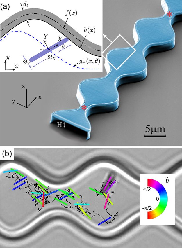
XIANG YANG et al.                                                                                 PHYSICAL REVIEW E 99, 020601(R) (2019)

    FIG. 3. (a) Average local diffusivity, Dave (x), plotted along the
                                                                                FIG. 4. (a) MFPT T (±x|0) vs x from experiments (sym-
channel for three rods with lX = 1, 1.2, and 1.6 μm [see correspond-
                                                                            bols) and theory (curves) in thin channels (H = 1.0 μm, α = 78 ) for
ing numerical results in Fig. S3(c)]. (b) Tilting angle distributions
                                                                            different values of the pair (hn , lX ). Inset: vertical dashed segments
in the neck regions (x = ±L/2, symbols), and at the center of the
                                                                            mark the starting (x = 0, red) and ending (x = ±x, blue) positions
channel cell (x = 0, dashed lines), for the same lX as in (a). Data
                                                                            of the recorded first-passage events. (b) MFPT at x = L/2 vs
were taken in a tall channel (H = 2.0 μm, α = 1) with hn = 1.4 μm.
                                                                            hn /lX , measured in tall channels (H = 2.0 μm, α = 1) for different
                                                                            hn and lX . Results from experiments and theory are represented by
of Fig. 2(b) to a quasi-2D channel with half-width G(x),                    circles and crosses, respectively; symbols are color-coded according
adopted Reguera-Rubí expression [19,20,42], and arrived at                  to the actual value of lX . The local diffusivity, Dave (x), used in the
the following estimate for D(x):                                            theoretical computations was obtained via finite-element analysis
                                  Dave (x)                                  (see Supplemental Material Sec. II A [36]). The dashed line is a guide
                    D(x) =                      .                     (4)   to the eye.
                              [1 + G (x)2 ]1/3
The validity and corresponding implications of Eq. (4) are
discussed in Supplemental Material Sec. II A [36].                          region. In addition, the validity of our generalized FJ equa-
    Mean first-passage times. With both the entropic poten-                 tion has been systematically explored by extensive Brownian
tial, − ln G(x)/G(0), and the effective logitudinal diffusiv-               dynamics simulations in Supplemental Material Sec. I D [36].
ity, D(x), as extracted from the experimental data, one can                     Our experiments were controlled by two geometric pa-
next apply the FJ equation to analytically study the diffusive              rameters: the half-width of the channel’s necks, hn , and the
dynamics of confined rods. For example, we focus on the                     rod half-length, lX . Numerical and experimental results in
time duration, T (±x|0), of the unconditional first-passage                Fig. 4 clearly reveal that the MFPT increases as the ratio
events that start at x = 0 and end up at x = ±x [see inset                 hn /lX decreases. Moreover, provided that the rods are not too
of Fig. 4(a)], regardless of the fast-relaxing coordinates y                short, lX > 0.8 μm, results for different choices of hn and lX ,
and θ . The corresponding MFPT, T (±x|0), can then be                    when plotted versus hn /lX , collapse onto a universal curve, as
used to estimate the asymptotic channel diffusivity in narrow-              illustrated in Fig. 4(b). This means that, in the experimental
neck cases, i.e., Dch = limt→∞ [x(t ) − x(0)]2 /2t, that is,              regime investigated here, proportional increases of hn and lX
Dch = L 2 /2T (±L|0) [5]. Taking advantage of the symmetry                do not change the MFPT. For a qualitative explanation of such
properties of the system, Eq. (3) returns an explicit integral              a property, we notice that increasing lX reduces the available
expression for the MFPT [19,43], reading                                    configuration space and, simultaneously, raises the relevant
                                  x
                                          dη          η                     entropic barriers [Fig. 2(d)]. As a consequence, longer rods,
        TF J (±x|0) =                                  G(ξ )dξ .   (5)   which also possess smaller diffusivity, D(x) [Fig. 3(a)], tend
                              0        G(η)D(η)   0                         to diffuse with longer MFPT’s. On the other hand, increasing
In Fig. 4(a) we compare the predictions of Eq. (5) with the                 hn lowers the entropic barrier, thus decreasing the MFPT. As
experimental measurements of T (±x|0) for six combina-                   quantitatively discussed in Supplemental Material Sec. II C
tions of hn and lX . Without any adjustable parameters, Eq. (5)             [36], these two opposite effects tend to compensate each other,
yields predictions in excellent agreement with the experimen-               in our experimental regime, as long as the ratio hn /lX is kept
tal data and captures the fast increase of the MFPT in the neck             constant.

                                                                      020601-4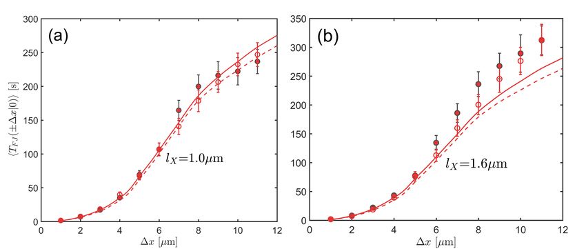
DIFFUSION OF COLLOIDAL RODS IN CORRUGATED …                                                 PHYSICAL REVIEW E 99, 020601(R) (2019)

   In conclusion, we experimentally measured diffusive trans-          and, similarly to the colloidal rods in our experiments, their
port of colloidal rods through corrugated planar channels,             description would generally require higher dimensional con-
upon systematically varying the geometric parameters of the            figuration spaces. However, as in our work, fast relaxing
rods and the channel. Anisotropic shape significantly impacts          d.o.f.’s (“perpendicular” to the channel direction) may be
particle transport by altering free-energy barriers and parti-         adiabatically eliminated and replaced by a reduced free-
cle diffusivity. Experimental observations were successfully           energy potential [Fig. 2(d)] together with an effective diffu-
modeled by generalizing the FJ theory for spherical particles          sivity function [Eq. (4) and Fig. 3(a)]. Such a generalization
in terms of an effective longitudinal diffusivity, with hydro-         of the FJ approach consequently may serve as a powerful
dynamic and entropic adjustments, and an FJ free energy                phenomenological tool to accurately describe the diffusive
including the rotational d.o.f.                                        transport of real-life particles in directed corrugated narrow
   Our method to quantify particle-shape-induced entropic              channels.
effect [cf. Fig. (2)] is also applicable to model the con-                Acknowledgments. We acknowledge financial support from
fined diffusion of even more complex particles, like patchy            the NSFC (Grants No. 11774222, No. 11422427, and
colloids [28] or polymers [29,30]. Such particles possess              No. 11402069) and the Program for Professor of Special
additional d.o.f.’s, other than the pure translational ones,           Appointment at Shanghai Institutions of Higher Learning.

 [1] B. Berkowitz, A. Cortis, M. Dentz, and H. Scher, Rev. Geophys.    [26] D. Kasimov, T. Admon, and Y. Roichman, Phys. Rev. E 93,
     44, RG2003 (2006).                                                     050602 (2016).
 [2] M. J. Skaug, L. Wang, Y. F. Ding, and D. K. Schwartz, ACS         [27] F. Hofling, E. Frey, and T. Franosch, Phys. Rev. Lett. 101,
     Nano 9, 2148 (2015).                                                   120605 (2008).
 [3] C. Kettner, P. Reimann, P. Hänggi, and F. Müller, Phys. Rev. E    [28] S. Sacanna and D. J. Pine, Curr. Opin. Colloid Interface Sci. 16,
     61, 312 (2000).                                                        96 (2011).
 [4] S. Matthias and F. Müller, Nature (London) 424, 53 (2003).        [29] N. Fakhri, F. C. MacKintosh, B. Lounis, L. Cognet, and M.
 [5] X. Yang, C. Liu, Y. Li, F. Marchesoni, P. Hänggi, and H. P.            Pasquali, Science 330, 1804 (2010).
     Zhang, Proc. Natl. Acad. Sci. USA 114, 9564 (2017).               [30] A. Ward, F. Hilitski, W. Schwenger, D. Welch, A. W. C. Lau,
 [6] M. J. Skaug, C. Schwemmer, S. Fringes, C. D. Rawlings, and             V. Vitelli, L. Mahadevan, and Z. Dogic, Nat. Mater. 14, 583
     A. W. Knoll, Science 359, 1505 (2018).                                 (2015).
 [7] F. Slanina, Phys. Rev. E 94, 042610 (2016).                       [31] W. Reisner, K. J. Morton, R. Riehn, Y. M. Wang, Z. Yu, M.
 [8] H.-X. Zhou, G. Rivas, and A. P. Minton, Annu. Rev. Biophys.            Rosen, J. C. Sturm, S. Y. Chou, E. Frey, and R. H. Austin,
     37, 375 (2008).                                                        Phys. Rev. Lett. 94, 196101 (2005).
 [9] P. C. Bressloff and J. M. Newby, Rev. Mod. Phys. 85, 135          [32] W. Riefler, G. Schmid, P. S. Burada, and P. Hänggi, J. Phys.:
     (2013).                                                                Condens. Matter 22, 454109 (2010).
[10] P. Hänggi and F. Marchesoni, Rev. Mod. Phys. 81, 387 (2009).      [33] C. Bechinger, R. Di Leonardo, H. Löwen, C. Reichhardt, G.
[11] P. S. Burada, P. Hänggi, F. Marchesoni, G. Schmid, and P.              Volpe, and G. Volpe, Rev. Mod. Phys. 88, 045006 (2016).
     Talkner, Chem. Phys. Chem. 10, 45 (2009).                         [34] C. Liu, C. Zhou, W. Wang, and H. P. Zhang, Phys. Rev. Lett.
[12] O. Benichou and R. Voituriez, Phys. Rep. 539, 225 (2014).              117, 198001 (2016).
[13] F. Hofling and T. Franosch, Rep. Prog. Phys. 76, 046602 (2013).   [35] J. C. Wu, Q. Chen, R. Wang, and B. Q. Ai, Chaos 25, 023114
[14] W. M. Deen, AIChE J. 33, 1409 (1987).                                  (2015).
[15] B. Hille, Ion Channels of Excitable Membranes (Sinauer Asso-      [36] See Supplemental Material at http://link.aps.org/supplemental/
     ciates, Sunderland, MA, 2001).                                         10.1103/PhysRevE.99.020601 for fabrication procedures, dif-
[16] J. Kärger and D. M. Ruthven, Diffusion in Zeolites and Other           fusion measurements, finite-element calculation, and Brownian
     Microporous Solids (Wiley, New York, 1992).                            dynamics simulations.
[17] M. Wanunu, T. Dadosh, V. Ray, J. M. Jin, L. McReynolds, and       [37] J. Happel and H. Brenner, Low Reynolds Number Hydrodynam-
     M. Drndić, Nat. Nanotechnol. 5, 807 (2010).                           ics (Prentice Hall, Englewood Cliffs, NJ, 1965).
[18] M. Jacobs, Diffusion Processes (Springer, New York, 1967).        [38] M. M. Tirado, C. L. Martínez, and J. G. de la Torre, J. Chem.
[19] R. Zwanzig, J. Phys. Chem. 96, 3926 (1992).                            Phys. 81, 2047 (1984).
[20] D. Reguera and J. M. Rubí, Phys. Rev. E 64, 061106 (2001).        [39] J. L. Bitter, Y. Yang, G. Duncan, H. Fairbrother, and M. A.
[21] P. Kalinay and J. K. Percus, Phys. Rev. E 74, 041203 (2006).           Bevan, Langmuir 33, 9034 (2017).
[22] D. Reguera, G. Schmid, P. S. Burada, J. M. Rubí, P. Reimann,      [40] M. Lisicki, B. Cichocki, and E. Wajnryb, J. Chem. Phys. 145,
     and P. Hänggi, Phys. Rev. Lett. 96, 130603 (2006).                     034904 (2016).
[23] A. M. Berezhkovskii, M. A. Pustovoit, and S. M. Bezrukov,         [41] Y. Han, A. Alsayed, M. Nobili, and A. G. Yodh, Phys. Rev. E
     J. Chem. Phys. 126, 134706 (2007).                                     80, 011403 (2009).
[24] Y. Han, A. M. Alsayed, M. Nobili, J. Zhang, T. Lubensky, and      [42] A. M. Berezhkovskii, L. Dagdug, and S. M. Bezrukov, J. Chem.
     A. Yodh, Science 314, 626 (2006).                                      Phys. 143, 164102 (2015).
[25] A. Chakrabarty, A. Konya, F. Wang, J. V. Selinger, K. Sun, and    [43] N. S. Goel and N. Richter-Dyn, Stochastic Models in Biology
     Q. H. Wei, Phys. Rev. Lett. 111, 160603 (2013).                        (Academic Press Inc., New York, 1974).

                                                                 020601-5
Supporting Information for                                Diusion of Colloidal Rods in Corrugated
                                                              Channels
                                                   1               1            1                 2
                            Xiang Yang,                Qian Zhu,       Chang Liu,    Wei Wang,        Yunyun

                                 3                       4, 5                       3, 6                     1, 7
                           Li,       Peter Hänggi,              Fabio Marchesoni,          and H. P. Zhang

                     1
                         School of Physics and Astronomy and Institute of Natural Sciences,

                                         Shanghai Jiao Tong University, Shanghai, China

                                           2
                                               School of Material Science and Engineering,

            Harbin Institute of Technology, Shenzhen Graduate School, Shenzhen,China

                                     3
                                         Center for Phononics and Thermal Energy Science,

                                               School of Physics Science and Engineering,

                                                  Tongji University, Shanghai, China

                 4
                     Institut für Physik, Universität Augsburg, D-86135 Augsburg, Germany

    5
        Nanosystems Initiative Munich, Schellingstrasse 4, D-80799 München, Germany

             6
                 Dipartimento di Fisica, Università di Camerino, I-62032 Camerino, Italy

        7
            Collaborative Innovation Center of Advanced Microstructures, Nanjing, China

                                                        (Dated:    November 24, 2018       )

                                                                    Abstract
  This document contains supporting information for the article entitled                                     Diusion of Col-
loidal Rods in Corrugated Channels

                                                                        1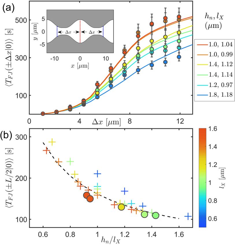
I. MATERIAL AND METHOD
A. Colloidal rod fabrication
Gold microrods were synthesized by electrodeposition in alumina templates following a
procedure adapted from an earlier study [1]. Porous AAO membranes (Whatman) with a
nominal pore diameter of 200 nm were used. Before electrodeposition, a 200 - 300 nm layer
of silver was thermally evaporated on one side of the membrane as the working electrode.
The membrane was then assembled into an electrochemical cell with the pore openings
immersed in the metal plating solution. Silver plating solution (Alfa Aesar) and homemade
gold solution (gold content 28.7 g/L) were used. In a typical experiment, a 5 - 10 µm
2
layer of silver was
rst electro-deposited into the pores at -5 mA/cm , followed by gold
2
at -0.2 mA/cm , the amount of which was controlled by monitoring the charge
ow. The
pores' silver
lling and the membrane were then dissolved, respectively in HNO3 and NaOH
solutions, and the released gold rods were cleaned in distilled water. In the
nal step of the
fabrication process, a thin layer (50 nm) of iron was then thermally evaporated by electron
beam in a vacuum onto the sides of the gold rods (e-beam evaporator HHV TF500). Rod
width is about 300 nm and we selected straight rods with length from 1.6 µm to 3.2 µm for
our experiment.
B. Local diusivity measurements
Con
ning boundaries cause the normal diusivity of the rods to spatially vary inside
the channel. We measured the local diusivity in the rod body frame DIJ (x, y, θ) (I, J =
X, Y, θ) via the displacement covariance matrix. As illustrated in Fig. S1(a) the elements of
the covariance matrix at a given sample point [marked by a cross in Fig. S1(c)] can be
tted
by linear functions of the elapsed time, δt, with slope proportional to the relevant diusivity
element, hδIδJi = 2DIJ (x, y, θ)δt (normal diusion). All non-diagonal cross-covariances,
such as hδX (δt) δY (δt)i shown in Fig. S1(a), are much smaller than the variances, which
means that the diusivity matrix DIJ (x, y, θ) is dominated by its diagonal elements. In
Fig. S1(b) all displacements after a time interval δt =0.2 s exhibit a normal Gaussian
distribution, which suggests that our choice of δt was appropriate. We carried out local
diusivity measurements at 200 points uniformly distributed in the con
guration space
2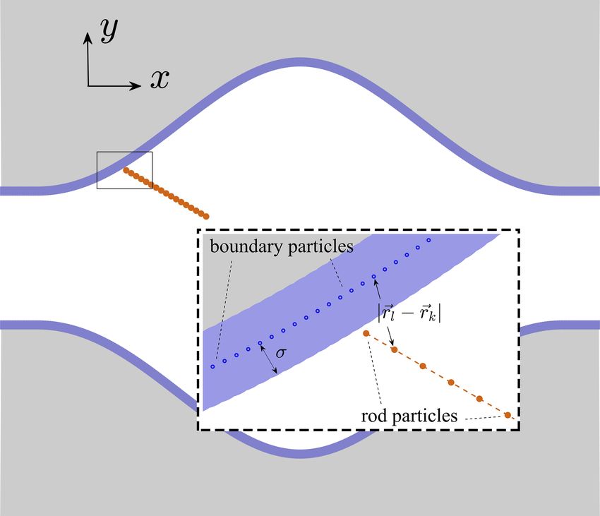
x, y, θ; then used such measurements to interpolate the diusivity matrix DIJ (x, y, θ) over
the entire parameter space. Measured DXX , DY Y , Dθθ for three tilting angles are depicted
in Figs. S1(c)-(e) see Fig. S3(a)-(b) for the corresponding numerical results.
C. Finite-element simulations
We complemented our experimental data for the local diusivity with
nite-element cal-
culations. COMSOL Multiphysics v5.2 was used to compute the drag force on a moving
rod in a channel. The Stokes equations were solved. In doing so, no-slip boundary condi-
tions were imposed on the side walls,
oor and ceiling, while open boundary conditions were
adopted for the channel openings. The geometry of the channel was set to reproduce the
inner channel boundary in the experiments. We used about half a million elements in the
simulation to ensure convergence. The same numerical method was followed to solve the
problem of a sphere moving in a long cylinder; the computed drag force on the sphere devi-
ates less than 3% from the analytical predictions [2], which can be regarded as an estimate
of the achieved numerical accuracy.
The rod dwells at dierent locations and orientations, (x, y, θ), in a horizontal plane at
about Hrod =0.4 µm above the
oor. We estimated Hrod by balancing the rod gravity (about
0.025 pN), buoyancy and the electrostatic repulsion between the rod and the channel walls,
for which we assume a Debye length of 60 nm and surface potentials of 40 mV [3, 4]. As
shown in Supporting Movie S1.mp4, the rods exhibit little out-of-plane motion; therefore,
in our simulations and experimental data analysis we assumed that they stay in the same
horizontal plane at all times.
For each (x, y, θ), we dragged the rod with constant velocity v = 1µm/s in the x or y
direction, and measured the corresponding drag force fx and fy in each case. We calculated
the hydrodynamic friction coe
cient matrix γ = {γij }, (i, j = x, y ) through the relation
f~ = γ~v . Then, the diusion matrix was derived from the γ matrix via the
uctuation-
dissipation theorem[5].
3Figure S1. (a) Covariances of linear and angular displacements, δX 2 , δY 2 , hδXδY i and δθ2
, versus elapsed time δt at coordinates: (x=-2.5 µm, y =1.6 µm, θ=π/4), marked by a cross in the
middle panel of (e). Linear
ts were used to extract the corresponding diusivity matrix element.
(b) Probability distributions of δX , δY , and δθ at δt = 0.2 s
tted by Gaussian functions (dashed
curves) with corresponding variance from panel (a). (c)-(e) Diagonal terms of the local diusivity
in the body frame (c) DXX (x, y, θ), (d) DY Y (x, y, θ) and (e) Dθθ (x, y, θ) are measured at θ = 0, π/4
and π/2. Data were taken in a tall channel with hn = 1.4µm and lX = 1µm; the channel's inner
boundaries ±h(x) are marked by solid lines.
4D. Brownian Dynamics (BD) simulations
Because the inertial forces are negligible with respect to the viscous forces, we used
overdamped Langevin equations to describe the evolution of rod coordinates and orientation,
denoted by the vector ~s = (x, y, θ):
d~s D(~s) ~ ~
= −R F (~s) + Rξ(t), (S1)
dt kB T
cos θ − sin θ 0
where R = sin θ cos θ 0 is the transformation matrix from the body to the laboratory
0 0 1
s) in the body frame contains diagonal elements only, DXX (~s),
frame. The diusion matrix D(~
DY Y (~s), Dθθ (~s), which are provided either by experimental measurements or
nite-element
simulations. Interaction force and torque between rod and boundary, F~ (~s), are computed in
the body frame (see below). Fluctuations in the body frame are independent Gaussian white
noises ~ ,
ξ(t) with hξI (t)i = 0 and hξI (t + τ )ξJ (t)i = 2DIJ (~s)δ(τ )δIJ , where I(J) represents
X, Y or θ, as appropriate.
We computed the rod-wall interaction in the following way. As illustrated in Fig. S2, the
channel boundary and the rod are represented by a string of particles: the l-th boundary
particle is denoted by r~l = (xl , yl ) and the k -th rod particle by ~rk . These particles interact
with each other via the truncated Lennard-Jones(LJ) potential rl − r~k |),
U (|~
ULJ (r) − ULJ (1.12σ), r ≤ 1.12σ
U (r) = (S2)
0, r > 1.12σ
σ σ
ULJ (r) = 4ε[( )12 − ( )6 ], (S3)
r r
where ε and σ are the strength and characteristic length of the potential respectively. Total
force and torque acting on the rod are combined in the vector
P
− ∇X U (|~
rl − ~rk |)
k,l
P
~
F (~s) =
− ∇Y U (|~
rl − ~rk |) ,
k,l
P
− |~
rl − ~r|∇Y U (|~
rl − ~rk |)
k,l
5where ~r = (x, y) denotes the center of the rod.
We had recourse to Euler's method to discretize the Langevin equations with time step dt.
For thermodynamic consistency, we used the transport (also known as kinetic or isothermal)
convention [68], and a predictor-corrector scheme [9] to compute the post-point value,
~s(t + dt). We
rst predict the post-point value from the information at ~s(t)
D(~s(t)) ~ p
~s∗ (t + dt) = ~s(t) + R F (~s(t))dt + R 2D(~s(t))dt~η (t), (S4)
kB T
and then improve it in a corrector step
D(~s∗ (t + dt)) ~ ∗ p
~s(t + dt) = ~s(t) + R F (~s (t + dt))dt + R 2D(~s∗ (t + dt))dt~η (t) (S5)
kB T
where the vector ~η (t) consists of three independent Gaussian random numbers with zero
mean and unit variance. Our numerical scheme produces uniformly distributed rods in the
accessible space as in the experiments, which validates the scheme itself.
In our simulations we used the time step dt = 0.2 ms, potential parameters σ = 0.1µm
and ε = 2kB T , and located the wall particles ~rk , so that the space accessible to the dif-
fusing rod was the same as in the experiments. Upon rescaling length, time, and energy
respectively by L, L2 /Dave (x = 0) [see Eq. (3) in the main text], and kB T , the dimensionless
simulation parameters became σ = 8 × 10⁻³ , dt = 4 × 10⁻⁷ , and ε = 2. Particle trajectories
from simulation can be analyzed by the same technique (see main text) adopted for their
experimental counterparts to determine the relevant MFPTs.
II. DISCUSSION
A. Local diusivity measurements for
nite-element simulations
Typical
nite-element calculation results for DXX (x, y, θ) and DY Y (x, y, θ) are plotted in
Fig. S3(a)-(b). Upon integrating DXX and DY Y , as prescribed in Eq. (3), we obtained the
local diusivity along the channel direction, Dave (x), plotted in Fig. S3(c). These numerical
results agree with their experimental counterpart of Fig. S1. For example, both experiments
and
nite-element calculations suggest that for long rods Dave (x) is largest at the center of
the neck. We systematically investigated this phenomenon in Fig. S3(d) over a wide range
6Figure S2. Schematic diagram of the channel and rod model used to compute the rod-wall inter-
actions in BD simulations. Fixed particles (located at ~rk , separated by 0.25σ ) mimicking the walls
are shown in blue and those mimicking the diusing rod (located at ~rl , separated by 0.8σ ) in or-
ange. The quantity σ is the characteristic length of the LJ potential (see text). Periodic boundary
conditions are imposed at the left and right openings.
of the channel width, hn , and rod length, lX . For rods with lX > 1.2 µm, Dave (x = L/2) is
greater than Dave (x = 0). As a comparison, we calculate the rod translational diusivity at
the center of the channel cells with θ = 0; namely, D0 = [DXX (0, 0, 0) + DY Y (0, 0, 0)]/2 and
in the unbounded space, Dbulk = (DXX + DY Y )/2. Numerical values for these quantities are
shown in the caption of Fig. S3.
B. Diusion time scales and the generalized FJ approach
With the typical geometric parameters (lX =1 µm, hn =1.4 µm, hw =4.2 µm and L =12
µm) adopted in our experiments, we estimated the characteristic diusion times in the x
(channel) direction, τx = L2 /2D0 ' 200 s; in the y direction, τy = h2 /2D0 ' 23 s (cell
center) and 3 s(neck); and for the rod's rotation τθ = (π/2)2 /2Dθθ ' 1.5 s. Therefore,
relaxation in the y and θ directions are much faster than in the channel direction, which
justi
es implementing the FJ approach. We also note that τθ
τy in most space except in
the neck region.
7Figure S3. Numerical diusivity results from
nite-element calculation. Local diusivity in the
body frame (a) DXX (x, y, θ) and (b) DY Y (x, y, θ) computed for θ = 0, π/4, π/2. (c) Average local
diusivity Dave (x) vs. x for three rods of dierent length, for which the diusivity at the center
of the channel was D0 = 0.36,0.34 and 0.24 µm2 /s, to be compared with the diusivity in the
unbounded space, Dbulk = 0.47, 0.42 and 0.34 µm2 /s (see supporting text for de
nitions). (d)
Values of [Dave (0) − Dave (L/2)]/D0 in the hn -lX plane. Data were taken in a tall channel (H =
2.0 µm, α = 1) with hn =1.4 µm, see Figs. S1(c)-(d) and 3(a) for the corresponding experimental
results.
C. Reguera-Rubì approximation for eective diusivity
According to the FJ approach, the adiabatic elimination of the transverse coordinates
leads to entropic corrections to the eective local diusivity. For a 2D channel with con
ning
boundaries at ±g(x), Reguera and Rubí (RR) proposed the following expression for the
1
eective diusivity: D(x) = D0 [1 + g 0 (x)2 ]− 3 , if g 0 (x) < 1 [10]. RR also provided a formula
for 3D axisymmetric channels with spatial d.o.f.'s only. However, their formula does not
apply to a generic 3D channel. We approximated the reconstructed 3D channel [Fig. 2(b)] to
a quasi-2D one with half-width G(x) and applied the improved RR approximation, D(x) =
− 31
Dave (x) [1 + G0 (x)2 ] . As shown in Figs. S4(a)-(b), such an approximation raises the
8Figure S4. MFPT from experiments (
lled symbols), BD simulations (open symbols) and FJ
predictions with (solid curves) or without the improved RR correction (dashed curves). Data were
taken in tall channels (H =2 µm, α = 1) with hn =1.4 µm for two dierent rod half-lengths, (a)
lX = 1.0 and (b) 1.6µm. In the BD simulations we made use of the experimentally measured
diusivity matrix.
theoretical estimates by some 5% (solid versus dashed curves). For a short rod, lX =1 µm,
theoretical predictions are consistent with both experimental and simulation results. For a
long rod, lX =1.6 µm, however, the RR formula underestimates both the experimental and
simulation results by ∼15% note that the experimental and numerical data sets agree with
each other for all values of lX . This may be understood by noticing that the reconstructed
3D channel for a long rod, see Figs. 2 (b)-(c), exhibits large variations along the θ axis and,
therefore, cannot be accurately represented by an averaged quasi-2D channel.
D. Dependence of the MFPT on channel neck width and rod length
The width of the channel's neck, hn , and the length of the rod, lX , aect the MFPT by
changing both the entropic barrier and the eective diusivity in Eq. (5). To clarify their
combined eect, we denote hTF J (±∆x|0)i by T (ω; ∆x), where ω represents either hn or lX ,
as appropriate, and rewrite Eq. (5) as
ˆ∆x
1
T (ω; ∆x) = λ(ω; η) dη, (S6)
Dave (ω; η)
0
9where
1 ˆx
[1 + G0 (ω; x)2 ] 3
λ(ω; x) = G(ω; ξ)dξ
G(ω; x)
0
depends only on the geometric properties of the system. To further advance our analysis, we
assume a weak x dependence of the local diusivity Dave (ω; x). This assumption allows us
´L
to replace Dave (ω; η) in Eq. (S6) with its average, D̄(ω) ≡ L1 0 Dave (ω; η)dη . Accordingly,
T (ω; ∆x) is approximated by
ˆ∆x
1
T0 (ω; ∆x) = λ(ω; η)dη.
D̄(ω)
0
We now take the partial derivative of the MFPT at ∆x = L/2 [see Fig. 4(b)], that is
ˆL/2 ˆL/2
∂T0 (ω; L/2) 1 ∂λ(ω; η) ∂
= dη + D̄(ω)−1 λ(ω; η)dη (S7)
∂ω D̄(ω) ∂ω ∂ω
0 0
´ L/2 ∂λ(ω;η) !
dη ∂
= T0 (ω; L/2) ´ 0L/2 ∂ω + D̄(ω) D̄(ω)−1 .
λ(ω; η)dη ∂ω
0
From this equation we immediately realize that a change in the system parameter ω generates
´ L/2 ∂λ(ω;η) ´ L/2
two contributions, an entropic term, eω (ω) = 0 ∂ω
dη/ 0 λ(ω; η)dη , and a diusion
term,
∂
uω (ω) = D̄(ω) ∂ω D̄(ω)−1 .
As hn and lX change proportionally by the amounts dlX and dhn , i.e. dlX /dhn = lX /hn ,
the total change of T0 reads
hn
dT0 = T0 [ulX + elX + (uhn + ehn )]dlX . (S8)
lX
We computed each of these terms numerically in a tall channel with dierent lX and hn .
For the diusive terms we used diusivity matrices from
nite-element calculations. All four
terms of Eq.(S8) and their sum are plotted in Fig. S5. An increase of the rod length lX leads
to less available con
guration space and higher entropic barriers [see Fig. 2 (c)], that causes
the MFPT to increase. Vice versa, increasing hn reduces the height of the entropic barrier
and thus decreases the MFPT. This corresponds to positive elX and negative ehn values in
Fig. S5(a). A longer rod is naturally characterized by smaller diusivity [see Fig. 3(a)] and
longer MFPT, which is consistent with a positive value of ulX in Fig. S5(b). Changes in
the neck width, hn , has a weak impact on the eective diusivity, as proven by the small
10uhn values in Fig. S5(b). Adding up all four terms yields a vanishing MFPT increment,
dT0 ∼ 0, for all data points in Fig. S5(c), except the two points encircled by a dashed
ellipse. These two outliers represent the case of two short rods, lX = 0.6, and 0.5µm in an
extremely narrow channel with hn =0.6 µm (i.e., comparable with the rod width 2lY =0.3
µm). Under these conditions, a change in hn can lead to large values of ehn and uhn , also
marked by dashed ellipses in Figs. S5(a)-(b).
III. DESCRIPTION OF SUPPORTING VIDEO
Supporting video (S1.mp4) shows a typical rod trajectory plotted on an optical image of
the channel. Rod orientation is reported according to a color-code. Some of these data have
been plotted in Fig. 1(b).
[1] W. Wang, T.-Y. Chiang, D. Velegol, and T. E. Mallouk, J. Am. Chem. Soc. 135, 10557 (2013).
[2] K. Misiunas, S. Pagliara, E. Lauga, J. R. Lister, and U. F. Keyser, Phys. Rev. Lett. 115,
038301 (2015).
[3] T. Y. Chiang and D. Velegol, Langmuir 30, 2600 (2014).
[4] J. Israelachvili, Intermolecular and Surface Forces (Academic Press, 2011).
[5] R. Kubo, Rep. Prog. Phys. 29, 255 (1966).
[6] P. Hänggi, Helv. Phys. Acta 51, 183 (1978).
[7] I. M. Sokolov, Chem. Phys. 375, 359 (2010).
[8] O. Farago and N. Gronbech-Jensen, Phys. Rev. E 89, 013301 (2014).
[9] N. Bruti-Liberati and E. Platen, Stochastics and Dynamics 08, 561 (2008).
[10] D. Reguera, G. Schmid, P. S. Burada, J. M. Rubí, P. Reimann, and P. Hänggi, Phys. Rev.
Lett. 96, 130603 (2006).
11Figure S5. Illustration of Eq. (S8): (a) entropic terms elX and (hn /lX )ehn , (b) diusive terms ulX
and (hn /lX )uhn , and (c) sum of all four terms plotted vs. hn /lX . Data points from the two shortest
rods are encircled by dashed ellipses (see text). All data points are color coded according to the
rod half-length, lX .
12You can also read