Optimal Physical Preprocessing for Example-Based Super-Resolution
←
→
Page content transcription
If your browser does not render page correctly, please read the page content below
Optimal Physical Preprocessing for
                                           Example-Based Super-Resolution
                                           A LEXANDER R OBEY             AND    V IDYA G ANAPATI *
                                           Swarthmore College, Engineering Department, 500 College Ave, Swarthmore, PA 19081
                                           * vganapa1@swarthmore.edu

                                           ganapati.swarthmore.edu

                                           Abstract: In example-based super-resolution, the function relating low-resolution images to
                                           their high-resolution counterparts is learned from a given dataset. This data-driven approach
arXiv:1807.04813v1 [eess.IV] 12 Jul 2018

                                           to solving the inverse problem of increasing image resolution has been implemented with deep
                                           learning algorithms. In this work, we explore modifying the imaging hardware in order to collect
                                           more informative low-resolution images for better ultimate high-resolution image reconstruction.
                                           We show that this “physical preprocessing" allows for improved image reconstruction with deep
                                           learning in Fourier ptychographic microscopy.
                                              Fourier ptychographic microscopy is a technique allowing for both high resolution and high
                                           field-of-view at the cost of temporal resolution. In Fourier ptychographic microscopy, variable
                                           illumination patterns are used to collect multiple low-resolution images. These low-resolution
                                           images are then computationally combined to create an image with resolution exceeding that of
                                           any single image from the microscope. We use deep learning to jointly optimize the illumination
                                           pattern with the post-processing reconstruction algorithm for a given sample type, allowing for
                                           single-shot imaging with both high resolution and high field-of-view. We demonstrate, with
                                           simulated data, that the joint optimization yields improved image reconstruction as compared
                                           with sole optimization of the post-processing reconstruction algorithm.
                                           © 2018 Optical Society of America

                                           1.   Introduction
                                           Deep learning, a subset of machine learning, has shown remarkable results in the interpretation of
                                           data. By computationally finding complex, higher-order patterns in labeled datasets, deep learning
                                           has yielded state-of-the-art results in areas such as the classification of images [1], language
                                           translation [2], and speech recognition [3]. Deep learning is powerful because the mathematical
                                           form of the relationship between the input and output need not to be specified beforehand; the
                                           deep learning algorithm can computationally find arbitrary, non-linear relationships in datasets.
                                              The “super-resolution" problem of converting low-resolution images to higher resolution has
                                           been attempted with machine learning [4–12]. The super-resolution problem is an ill-posed
                                           inverse problem, with many high-resolution images possible for a given low-resolution image. In
                                           example-based super-resolution, machine learning attempts to make the problem well-posed by
                                           applying prior information.
                                              In example-based super-resolution, the training inputs are low-resolution image patches, and
                                           the training outputs are the corresponding high-resolution image patches. Machine learning then
                                           attempts to find the function that takes the low-resolution patch as the input, and then outputs the
                                           high-resolution patch. Deep convolutional neural networks have been promising in tackling the
                                           super-resolution problem [5, 7, 8, 10, 11], and the addition of adversarial networks has resulted in
                                           improved image quality of fine details [9]. Example-based super-resolution with deep learning
                                           has also been applied to microscopy images [13–15]. The success of these super-resolution deep
                                           neural networks can be attributed to the fact that images are not random collections of pixels;
                                           images contain some structure. The more we constrain the category or type of images we use,
                                           the more structure the deep learning algorithm should be able to find.
                                              The desirability of obtaining a high-resolution image from low resolution stems from the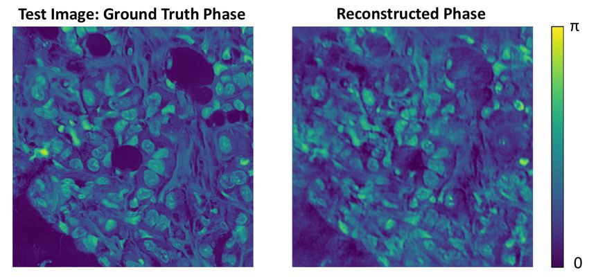
trade-offs inherent in designing imaging systems, due to constraints in physics and cost. The
minimum distance allowing two points to be distinguishable from each other determines the
resolution of an image; the lower the minimum distance, the higher the resolution. In the design
of an imaging system, resolution must be traded off with the total area imaged, the field-of-view.
We can obtain a low-resolution image with high field-of-view or vice versa. The tradeoff between
resolution and field-of-view of an imaging system can be quantified by its space-bandwidth
product [16]. Example-based super-resolution is a pathway to obtaining high resolution and high
field-of-view at the same time, i.e. a high space-bandwidth product.
   Another way to obtain a high space-bandwidth product is to trade off temporal resolution
by taking multiple images and stitching them together. This approach is undertaken in some
computational imaging modalities, where multiple image measurements are collected and
algorithmically combined.
   In the computational imaging paradigm, the imaging hardware is co-designed with the post-
processing software. In computational imaging, we do not attempt to collect an image directly.
Instead, we collect measurements that are used to create the image in post-processing. The
individual measurements do not necessarily resemble the final image, but they contain the
information necessary for image reconstruction. The data collected by the image sensor may be a
garbled version of the desired final image, requiring considerable computational post-processing,
sometimes with an iterative algorithm. The image reconstruction process from the collected noisy
sensor data is an inverse problem and may be ill-posed. Computational imaging modalities include
fluorescence imaging such as stochastic optical reconstruction microscopy [17], photoactivated
localization microscopy [18, 19] and structured light microscopy [20, 21], where multiple lower-
resolution images are computationally combined for a higher-resolution image without loss of
field-of-view. In computational imaging, we can also consider the problem of imaging the phase
of light, which cannot be measured directly. Fourier ptychographic microscopy is a modality
where multiple lower-resolution images are computationally combined for a higher-resolution
reconstruction of a complex object with both phase and amplitude [22].
   In Fourier ptychographic microscopy, the illumination source is a 2-dimensional matrix of
light-emitting diodes (LEDs). Low-resolution images with high field-of-view are collected by
illuminating the sample with different patterns of LEDs. The different illumination patterns
cause different spatial frequencies to be modulated into the pass-band of the optical system.
These low-resolution images are then computationally combined to create a high-resolution
reconstruction of the phase and amplitude of the sample, preserving the field-of-view of the
low-resolution images. An iterative algorithm is generally used for the reconstruction, but can be
computationally intensive. Recently, deep learning has been used to solve the inverse problem
in several computational imaging modalities, replacing iterative methods [23–38], including in
Fourier ptychographic microscopy [39].
   Though Fourier ptychographic microscopy achieves a high space-bandwidth product, temporal
resolution is sacrificed: many low-resolution images need to be collected for reconstruction.
This makes imaging of dynamic processes, such as those in live cells, difficult. Imaging of such
processes requires sophisticated hardware control to rapidly acquire the low-resolution image
stack [40].
   An emerging application for deep learning is to learn how to both optimally collect and
process data for some end goal, rather than just process data [41–45]. With this “physical
preprocessing" procedure for deep learning, data acquisition time or hardware requirements can
be reduced. In this work, we use deep learning to jointly optimize the illumination pattern in
Fourier ptychographic microscopy with the reconstruction algorithm for a given sample type,
allowing for single-shot imaging with a high space-bandwidth product. Our deep learning
algorithm looks for the illumination pattern that will embed the most information into a single
low-resolution image, along with a direct reconstruction method to non-iteratively reconstruct
the high-resolution complex field from the single image measurement.

2.   Background on Fourier Ptychographic Microscopy
In Fourier ptychographic microscopy, a sample is illuminated by a light-emitting diode (LED), as
in Fig. 1. We assume that the LED is sufficiently far away that the light entering the sample can
be approximated as a plane wave. The sample scatters the entering plane wave, and the exiting
wave is imaged through a microscope objective with a given numerical aperture (NA).

                                                   LED Matrix

                                                     Sample

                                                    Objective

Fig. 1: Schematic of Fourier ptychographic microscope setup. An LED matrix replaces the
illumination source of a traditional microscope.

    Consider a thin sample that is in the xy-plane and centered at the origin in in the Cartesian
coordinate system shown in Fig. 2. The illuminating LED is placed at the point (xl, yl, zl ). The
spatial profile of the plane wave from the LED entering the sample is described by ei2π u®l ·®r where
u®l · x̂ = ul, x is the spatial frequency in the x-direction and u®l · ŷ = ul,y is the spatial frequency in
the y-direction. The vector u®l is in the direction of −xl x̂ − yl ŷ − zl ẑ. The magnitude of u®l is
| u®l |= λ1 , where λ is the wavelength of the light. From Fig. 2, we see the following:
                                      1                     xl
                             ul, x = − sin θ cos φ = − q                ,                               (1)
                                      λ
                                                      λ xl2 + yl2 + zl2

                                      1                    yl
                              ul,y = − sin θ sin φ = − q               .                                (2)
                                      λ
                                                      λ xl + yl2 + zl2
                                                         2

  We use the thin transparency approximation to describe the sample as a complex transmission
function o(x, y). The field immediately after the sample can be described as the object transmission
function multiplied by the illumination plane wave at z = 0:

                                         o(x, y)ei2π (ul, x x+ul, y y ) .                               (3)

   If the 2D Fourier transform of o(x, y) is given as O(u x, uy ), the field in Eqn. 3 in Fourier space
is simply a shift, O(u x − ul, x, uy − ul,y ). The field is multiplied in Fourier space by the pupil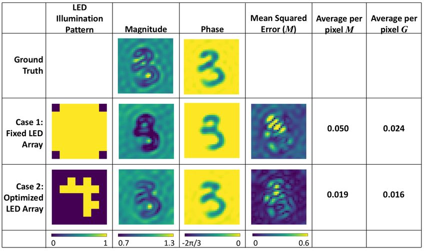
z

                                                          zl

                                                               φ

                                                          θ
                                                                                            y
                                                                                yl

                                     xl

                    x

Fig. 2: The light from an LED at point (xl, yl, zl ) illuminating a sample centered at the origin can
be approximated as a plane wave with spatial frequencies given by Eqn. 1 and Eqn. 2.

function of the objective, P(u x, uy ), a low-pass filter. In the case of no aberrations, P(u x, uy ) is
unity within a circle with radius NA
                                   λ , and zero elsewhere. The image sensor records the intensity
I of this field in real space:

                             I =| F −1 {P(u x, uy )O(u x − ul, x, uy − ul,y )} | 2,                 (4)
where F −1 denotes the inverse 2D Fourier transform [46, 47]. Due to the low-pass filtering
operation, the intensity image contains information from only a portion of spatial frequencies of
the original object.
   The previous discussion assumes illumination from a single LED, where it is assumed that the
LED emits a coherent wave. In an array of LEDs, with multiple LEDs illuminated, we assume
that each LED emits a coherent wave that is mutually incoherent with the waves emitted from the
other LEDs. Thus, if we have an matrix of LEDs in the xy-plane at height zl , the intensity image
recorded is:
                             n
                             Õ
                        I=         cl | F −1 {P(u x, uy )O(u x − ul, x, uy − ul,y )} | 2,           (5)
                             l=1

where n is the total number of illuminated LEDs and cl is the intensity of LED l [46].
   In the original instantiation of Fourier ptychographic microscopy, the LEDs are turned on and
off one at a time, generating n intensity images [22]. Other work uses a series of patterns of
illuminated LEDs, reducing the total number of images needed [40, 46]. Adaptive schemes can
also reduce the required number of LED images [48].
   The goal of Fourier ptychographic microscopy is to reconstruct the sample’s complex trans-
mission function, o(x, y) from these intensity images. A variety of iterative approaches have
been applied to the reconstruction process [47]. The creation of each intensity image involves
frequency modulation and a low-pass filtering operation. Each intensity image has limited
spatial bandwidth, but reflects information from a different portion of frequency space. Thus, the
reconstructed o(x, y) in Fourier ptychographic microscopy can have higher spatial bandwidth
than that specified by the NA of the objective.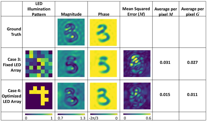
Though Fourier ptychographic microscopy creates images with a high space-bandwidth
product, it requires acquisition of multiple images. In this work, we aim to enable Fourier
ptychographic microscopy with single image acquisition, using a deep learning approach to
jointly find the optimal illumination pattern and reconstruction procedure for a given sample
type. Our reconstruction procedure replaces previously used iterative methods with a deep neural
network.

3.   A Communications Approach
Claude Shannon’s fundamental work in the theory of communication forms a framework to
circumvent the loss of temporal resolution in Fourier ptychographic microscopy. We consider the
problem of imaging a live biological specimen and model the Fourier ptychographic microscope
as a communication system, as shown in Fig. 3. In a general communication system, a message
from an information source is encoded, transmitted over a noisy channel, and decoded by a
receiver. If we know the statistics of the source, and the noise characteristics of the channel,
we can optimize the method of encoding and decoding for information transmission [49]. This
communications approach to imaging has been previously explored in [50].

Fig. 3: The general communication system in [49] applied to imaging a thin biological specimen.

   In the case of Fourier ptychographic microscopy, a biological sample is the information source,
and the message is the sample’s phase and amplitude (i.e. its complex transmission function) at a
point in time. The message is encoded as an optical signal by the pattern of illuminated LEDs.
This optical signal is then transmitted through the optics of the microscope. The image sensor of
the microscope camera receives the signal as intensity measurements over an array of sensor
pixels. The received signal may be corrupted by noise, such as Poisson noise. Finally, this image
sensor measurement must be decoded with an algorithm to try to reconstruct the original phase
and amplitude of the sample.
   In Fourier ptychographic microscopy, as in most imaging modalities, generally no assumptions
are made on the sample being imaged. Except in some cases [47], the imaging procedure of
acquiring low-resolution intensity images and solving for the high-resolution complex object
remains invariant with regards to the sample. However, the communication framework in
Fig. 3 yields insight on how to reduce the time needed to obtain high space-bandwidth complex
objects. If we can determine the statistics of the sample’s phase and amplitude “messages,"
it might be possible to compress all the information needed for reconstruction of the message
into a single image sensor measurement. This physical compression may be achieved by
choosing the optimal LED illumination pattern. We think of the sample as having a range of
different geometrical configurations, and optimizing a communication system for transmitting
and receiving information regarding the current configuration.
   Consider the following simple thought experiment. Imagine a sample having 2 possible states
that lead to 2 different phase and amplitude images. With a standard Fourier ptychographic
microscope, we would have to take multiple intensity images and complete the iterative
reconstruction procedure. However, only 1 bit of information needs to be transmitted and received
in this hypothetical system. Intuitively, the standard procedure is wasteful in this simple case; we
should easily be able to design an imaging system that only needs a single-shot measurement to
find the current state.
   There are two major difficulties in the implementation of a communications approach to
biological imaging. First, we need to determine the probability distribution of our “messages,"
which we need to discover through observations of the biological sample. Second, we need to
encode our messages for transmission, but we cannot choose an arbitrary encoding algorithm.
We are constrained to what is physically possible with optics.
   To solve these problems, we turn to deep learning to optimize the end-to-end communications
system, as in [51, 52], simulating the entire end-to-end imaging pipeline as a deep neural network.
During training of the network, the hardware parameters for encoding and the software parameters
for decoding are optimized. In the training process, the neural network takes high-resolution
complex objects obtained from a standard Fourier ptychographic microscope as input. From
the input complex object, the low-resolution image collected with a single LED illumination
pattern is emulated. This single low-resolution image then passes through post-processing neural
network layers, outputting a prediction of the high-resolution complex object. The illumination
pattern and the parameters of the post-processing layers are optimized during training, using
a dataset of high-resolution complex objects from a given sample type, as diagrammed in
Fig. 4. In the evaluation phase, we implement the optimized illumination in the actual Fourier
ptychographic microscope. Each collected single low-resolution image is then fed directly into
trained post-processing layers to reconstruct the high-resolution complex object (see Fig. 4).
With this procedure, we could use fixed biological samples to collect the training dataset, and live
samples in the evaluation step, potentially enabling unprecedented imaging of dynamic biological
processes.

           Fig. 4: Outline of the training and evaluation of the deep neural network.

4.   Methods
We implement the structure shown in Fig. 4 as a computational graph, and optimize the parameters
with TensorFlow [53], an open-source Python package for machine learning. We utilized
computational resources from the Extreme Science and Engineering Discovery Environment
(XSEDE) [54] for training of the computational graph. We include the simulation of the optical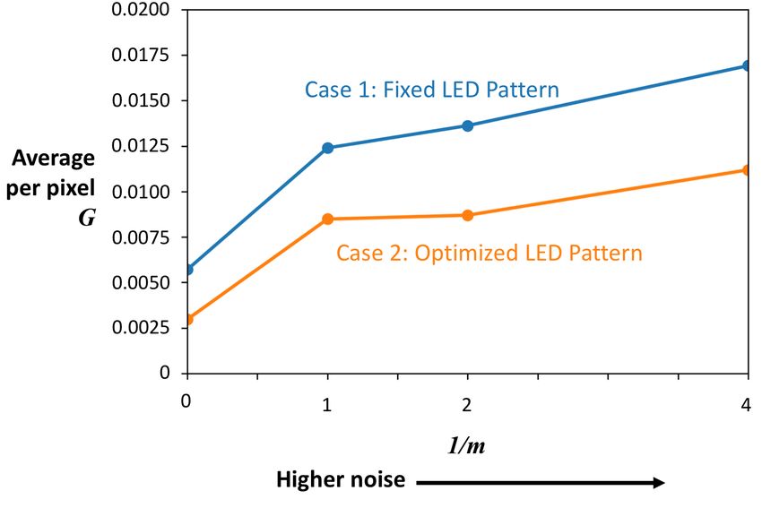
function to go from the high-resolution complex object to the low-resolution collected image in
the first layers of the deep neural network graph. The latter layers of the deep neural network
graph aim to transform the simulated low-resolution image back to the high-resolution complex
field, replacing an iterative algorithm. The first “physical preprocessing" layers emulate the
function of the optics, and allow the parameters of the actual physical system to be optimized
at the same time as the reconstruction algorithm. An overview of our computational graph is
shown in Fig. 5.

 Fig. 5: Overview of our computational graph that is trained with a dataset of input examples.

  We utilize computationally simulated datasets for training and testing of the deep neural
network. The dataset is composed of high-resolution, high field-of-view complex objects,
emulating those reconstructed from a standard Fourier ptychographic microscope setup. To
create the complex phase and amplitude images, we take datasets of intensity images and turn
them into complex objects. Our first example dataset takes the MNIST dataset of handwritten
digits [55] and turns it into a complex object dataset by applying the following formula to each
pixel:
                                                π
                                            e−i 2 p0 ,                                        (6)
where p0 is a pixel of the original image. We then low-pass filter the complex field with the
synthetic NA associated with the Fourier ptychographic setup. The resulting complex objects are
the inputs to the computational graph in Fig. 5.
   The low-resolution intensity image corresponding to a single LED illumination pattern, Ilow ,
is computationally emulated by the procedure outlined in [46], summarized in Section 2. We
assume a square grid LED matrix where the intensity of the LED can be tuned from 0 to 1,
0 ≤ cl ≤ 1. We emphasize that these physical preprocessing layers are included in the TensorFlow
computational graph so that cl is optimized during the training process.
   The next layers of the computational graph add a Gaussian approximation of Poisson noise to
Ilow . Every pixel of Ilow is processed by:
                                   √
                                      Ilow × m × g + Ilow × m

                               max                            ,0 ,                            (7)
                                                 m
where m is a multiplicative factor chosen to fit the noise of a particular setup and g is drawn
from a normal random distribution. A higher m corresponds to higher signal-to-noise ratio. We
redraw the value of g at every evaluation of the TensorFlow computational graph.
   The noisy Ilow is the input to 2 separate post-processing networks. One network aims to
reproduce the real part of the high-resolution object and the other network aims to reproduce the
imaginary part, as shown in Fig. 5. The architecture for the networks is inspired by [56], and
shown in Fig. 6. Each convolutional layer in Fig. 6 is diagrammed in Fig. 7. The networks make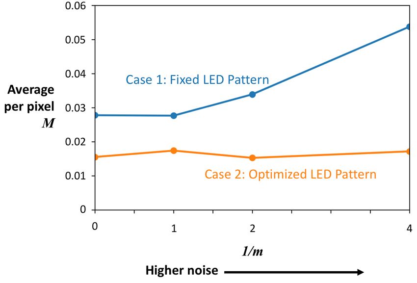
use of convolutional layers [57], maxout neurons [58], batch normalization [59], residual layers [1],
and dropout [60]. The outputs of the two neural networks, Ihighr e al and Ihighi mag , are combined
to output the high-resolution complex field reconstruction, e Ihigh = Ihighr e al + iIhighi mag .

Fig. 6: Diagram of the architecture inside the “ConvNet" blocks in Fig. 5. Each numbered square
in this diagram represents a convolutional layer with batch normalization and maxout neurons, as
shown in Fig. 7. The numbered squares correspond to kernel lengths of 10, 20, 30, 40, 50, 60,
70, 80 respectively. During training, 20% of the nodes in the layers in red are dropped out. Also
shown are the residual connections.

                      Fig. 7: Diagram of each convolution layer in Fig. 6.

   Generative adversarial networks have had success in mimicking the probability distribution of
a dataset [61], and the inclusion of a discriminative network has shown success in improving
image quality in super-resolution deep neural networks [9]. We include a discriminative network
that takes as input both eIhigh and the actual high-resolution field e
                                                                     Iactual and classifies whether
the input is an output of the reconstruction network (a “fake") or an actual high-resolution image,
as shown in Fig. 5. The objective function of this discriminative network is the cross-entropy
loss of correct classification. We alternate training the parameters of the discriminative network
to improve the cross-entropy loss with training of the rest of the computational graph to improve
the overall objective function.
   Our overall objective function consists of 3 parts, as in [62]:

                                         J = M + αG + C,                                         (8)
where M is the mean-squared error between e        Ihigh and eIactual , G is the mean-squared error
between the first gradients of Ihigh and Iactual , and C is the cross-entropy loss representing how
                                e         e
well the discriminative network is “fooled." In calculating G, we take the sum of the mean-squared
error of the gradient in the vertical direction and the gradient in the horizontal direction. The
gradient is calculated by taking the difference between e I and e
                                                                I shifted by one place. The metric C
measures how well the discriminative network is fooled, by calculating the cross-entropy loss of
                            Ihigh . The objective function includes the weighting factor α = 1, 000.
incorrect classification of e
   The parameters of the computational graph are trained with the Adam optimizer [63]. A
randomly selected batch of 4 high-resolution inputs e     Iactual from the training dataset are used
in every iteration of training. For each example in this work, we train for 100,000 iterations,
with a training rate of 1 × 10⁻² . The training rate is decayed by a factor of 0.99 every 1,000
iterations. The variable parameters of the computational graph are initialized with a truncated
normal distribution with σ = 0.1, and values limited to between 2 standard deviations from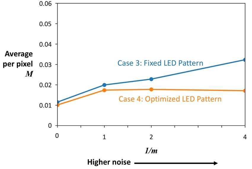
µ = 0. An exponential running average with decay rate of 0.999 of the variable parameters is
saved for testing.
5. Results and Discussion
We obtain image reconstruction results when we optimize the entire computational graph in
Fig. 5. We compare to the results when only optimizing the post-processing layers, keeping the
LED illumination pattern constant. As described in the previous section, the MNIST dataset of
intensity images is processed by Eqn. 6 and then low-pass filtered with the synthetic NA of the
Fourier ptychographic microscope. The optical parameters of the emulated Fourier ptychographic
microscope are given in Table 1. We utilize the full MNIST dataset, consisting of 55,000 training
images, 5,000 validation images, and 10,000 test images.
Size of high-resolution object 5.2 µm, 32 × 32 pixels
Wavelength of LED illumination 630 nm
NA of microscope objective 0.3
Magnification of microscope objective 10×
Pixel size of image sensor 6.5 µm
Pitch of LED matrix 4 mm
LED matrix size 7 x 7 grid, center 45 LEDs allowed to vary
Height of LED matrix, zl 25 mm
Synthetic NA of Fourier ptychographic microscope 0.80
Table 1: Optical parameters used for the simulated MNIST dataset; the original MNIST dataset
is padded with zeros to create 32 × 32 pixel images.
We train the following 4 cases of deep neural networks:
1. The LED matrix is fixed at constant, uniform illumination of cl = 1 for all l during training.
2. The LED matrix is initialized at constant, uniform illumination of cl = 1 for all l, but
allowed to change during training.
3. The LED matrix is fixed at a random initialization of cl , picked from a uniform random
distribution.
4. the LED matrix is initialized at the same random initialization of cl as in case (3), but is
allowed to vary during training.
Fig. 8 shows the results of the trained network for a randomly selected test example for cases
(1) and (2). In Fig. 8, the noise factor m = 0.25. From this single test example, we see that by
allowing the illumination pattern to vary, we obtain better results for both M, the mean-squared
error, and G, the mean-squared error of the image gradient. In Fig. 9, we vary m, and calculate
M and G averaged over the entire test dataset. Allowing the illumination pattern to vary yields
lower M and G for all the noise levels, with the difference growing greater for higher values of
1
m , corresponding to higher levels of noise. It appears that physical encoding of the data by the
illumination pattern allows for more robustness to noise.
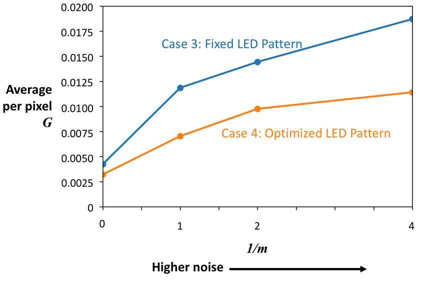
Fig. 10 shows the results for cases (3) and (4) for the same test example as in Fig. 8. We again
plot M and G averaged over the entire test dataset for different levels of noise in Fig. 11 forFig. 8: Test results for a single example for cases (1) and (2). The noise factor m = 0.25.
(a) M averaged over the test dataset for different m. (b) G averaged over the test dataset for different m.
Fig. 9: Cases (1) and (2).cases (3) and (4). We note similar trends to cases (1) and (2): allowing the LED pattern to vary
yields lower error. The final LED pattern in cases (2) and (4) are similar, even though the initial
conditions were different.
Fig. 10: Test results for a single example for cases (3) and (4). The noise factor m = 0.25.
Though the MNIST dataset is useful for fast prototyping, the images do not resemble biological
samples. In order to show proof-of-concept of this method for biologically relevant data, we
utilized breast cancer cell images from the UCSB Bio-Segmentation Benchmark dataset [64], and
converted the images to a high-resolution complex object dataset. Each image was cropped to
512 × 512 pixels and the three 8-bit color channels were summed. Each pixel p0 of the resulting
image was processed by:
i π (765−p0 )
e 765 , (9)
and then low-pass filtered by the synthetic NA of the Fourier ptychographic microscope. We used
34 images from the UCSB Bio-Segmentation Benchmark dataset for training and 12 images each
(a) M averaged over the test dataset for different m. (b) G averaged over the test dataset for different m.
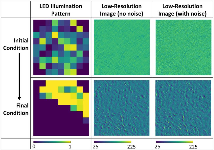
Fig. 11: Cases (3) and (4).for validation and testing. The optical parameters used for this dataset of images are summarized in Table 2. Size of high-resolution object 332.8 µm, 512 × 512 pixels Wavelength of LED illumination 630 nm NA of microscope objective 0.1 Magnification of microscope objective 5× Pixel size of image sensor 6.5 µm Pitch of LED matrix 4 mm LED matrix size 9 x 9 grid, center 69 LEDs allowed to vary Height of LED matrix, zl 100 mm Synthetic NA of Fourier ptychographic microscope 0.28 Table 2: Optical parameters used for the UCSB Bio-Segmentation Benchmark complex object dataset. Fig. 12 shows a test example after training a neural network with noise factor m = 1, following the considerations of case (4). We see reconstruction of many of the image details, and future work will focus on reducing the phase artifacts. Fig. 12: Test result for a single example for case (4) with the UCSB Bio-Segmentation Benchmark complex object dataset. The per pixel M and G for the reconstructed complex object are 0.112 and 0.014, respectively. Averaged over the entire training dataset, we have per pixel M = 0.190 and G = 0.016. Fig. 13b illustrates how the illumination pattern changed during training. The corresponding low-resolution images are also shown, with and without noise for the single validation example shown in Fig. 13a. Visually, we see enhanced image contrast in the low-resolution image corresponding to the final illumination pattern. In the initial low-resolution image, the image contrast is almost totally obscured with the addition of noise. When we compare the low-resolution images with noise in Fig. 13b, it appears that more information about the original object is preserved the final image, corresponding to the optimized illumination pattern. We hypothesize that optimizing the illumination pattern increases the mutual information of the low-resolution image and high-resolution complex object.
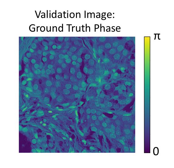
(a) Example validation object phase.

(b) LED matrix and corresponding low-resolution images for the validation object, at the beginning and end
of training.

   We perform a simple experiment to determine if the mutual information increases as we train
the deep neural network. We create a high-resolution dataset of 16 distinct images of 4 × 4 pixels.
Each image is a pattern of ones and zeros and each pixel is processed by Eqn. 6 and filtered by
the synthetic NA of the Fourier ptychographic microscope. An example complex object of this
dataset is shown in Fig. 14. The optical parameters used for this dataset are given in Table 3.
Given the optical parameters, each 4 × 4 pixel high-resolution complex object becomes a 1 × 1
pixel low-resolution intensity image.
   We trained 2 neural networks with no dropout, a batch size of 16, and noise level m = 1,
following the considerations of case (2) and case (4). The high-resolution dataset contains
log2 16 = 4 bits of information. For the low-resolution image to capture all the information about
the high-resolution dataset, the mutual information needs to be 4 bits. We calculate the mutual
information for the initial and final illumination patterns of both neural networks, as shown in
Fig. 15. The mutual information is calculated by:
Fig. 14: An example complex object in the 16 image, 4 × 4 pixel dataset.

      Size of high-resolution object                                 0.65 µm, 4 × 4 pixels
      Wavelength of LED illumination                                 630 nm
      NA of microscope objective                                     0.8
      Magnification of microscope objective                          10×
      Pixel size of image sensor                                     6.5 µm
      Pitch of LED matrix                                            8 mm
      LED matrix size                                                3 x 3 grid, all 9 LEDs allowed to vary
      Height of LED matrix, zl                                       10 mm
      Synthetic NA of Fourier ptychographic microscope               1.29

               Table 3: Optical parameters for the 16 image, 4 × 4 pixel dataset.


                                   ÕÕ                               p (x, y)
                                               p (x, y) log2                   ,                              (10)
                                   y ∈Y x ∈X
                                                                   p(x)p(y)

where p(x) is the marginal probability distribution of high-resolution objects, p(y) is the marginal
probability distribution of low-resolution images, and p(x, y) is the joint probability distribution.
For every x ∈ X, we use Eqn. 7 to generate 1,000,000 samples of y and approximate the
distribution p(y | X = x).
   From Fig. 15, we see that in our joint optimization procedure of the illumination pattern
and the post-processing parameters, the mutual information of the low-resolution image and
high-resolution object increases. We also note that the final LED illumination patterns are similar
for cases (2) and (4). It appears that during training, the LED illumination pattern changes so that
more information about the high-resolution object is physically encoded in the low-resolution
image. The physical preprocessing step is crucial to improved final complex object reconstruction.

6.   Conclusions
The success of deep learning presents an opportunity in the design of imaging systems: by finding
generalizable structure in past data, it is possible to figure out how to optimally collect future
data. This work uses deep learning to jointly optimize the physical parameters of the imaging
system together with the parameters of the image post-processing algorithm. We consider the
optimization of Fourier ptychographic microscopy and demonstrate that we can eliminate the
tradeoff among spatial resolution, field-of-view, and temporal resolution for a given sample type.
   This work frames the task of imaging a high-resolution complex field as a communications
problem, where image information is: (1) encoded as an optical signal with the programmable
(a) Case (2). (b) Case (4). Fig. 15: Mutual information of the high-resolution object and low-resolution image at the beginning and end of training. illumination source of a Fourier ptychographic microscope, (2) collected by an image sensor, and (3) computationally decoded. With a training dataset of high-resolution phase images of fixed cells, the parameters of both the microscope and the decoding algorithm can be co-optimized to maximize imaging speed. The optimized microscope can then be implemented to image the live sample, and the collected measurements fed directly into the post-processing layers of the computational graph, allowing for a high single-shot space-bandwidth product. With this method, instead of collecting images in the traditional sense, we optimally collect information about the spatial structure of the live sample. By using prior knowledge gained from static images, we avoid redundancy in information collection by physically preprocessing the data. We present results from simulated data, in order to show the feasibility of this method. Future work is needed to validate these methods with real experimental data. Additionally, our work assumes that the probability distribution of the training data matches the probability distribution of the test data. It is possible that the structure of the fixed samples may not be the same as the live samples. A possible method to alleviate this problem is to feed the output of the deep neural network into an iterative solver to ensure a valid solution to the inverse problem. Finally, we do not consider temporal relationships between images in this work. We consider each image frame as independent, however there is clearly a relationship between sequential frames. With a training set of video sequences, these temporal relationships could be accounted for. The framework outlined in this paper is not specific to Fourier ptychographic microscopy; these ideas can be extended to other imaging modalities with programmable parameters. Though we have focused on the benefits of this method for imaging of live biological samples, other benefits include reduced data storage needs and faster imaging for high-throughput studies. Acknowledgments This work used the Extreme Science and Engineering Discovery Environment (XSEDE) XStream at Stanford University through allocation TG-TRA100004. XSEDE is supported by National Science Foundation grant number ACI-1548562. The authors would like to thank Eden Rephaeli for coining the term “physical preprocessing."
References
1. K. He, X. Zhang, S. Ren, and J. Sun, “Deep residual learning for image recognition,” in The IEEE Conference on
    Computer Vision and Pattern Recognition (CVPR), (2016).
2. I. Sutskever, O. Vinyals, and Q. V. Le, “Sequence to Sequence Learning with Neural Networks,” in Advances in
    Neural Information Processing Systems 27, Z. Ghahramani, M. Welling, C. Cortes, N. D. Lawrence, and K. Q.
    Weinberger, eds. (Curran Associates, Inc., 2014), pp. 3104–3112.
3. G. Hinton, L. Deng, D. Yu, G. E. Dahl, A. r. Mohamed, N. Jaitly, A. Senior, V. Vanhoucke, P. Nguyen, T. N. Sainath,
    and B. Kingsbury, “Deep Neural Networks for Acoustic Modeling in Speech Recognition: The Shared Views of Four
    Research Groups,” IEEE Signal Process. Mag. 29, 82–97 (2012).
4. W. Freeman, T. Jones, and E. Pasztor, “Example-based super-resolution,” IEEE Comput. Graph. Appl. 22, 56–65
    (2002).
5. J. Kim, J. K. Lee, and K. M. Lee, “Deeply-Recursive Convolutional Network for Image Super-Resolution,”
    arXiv:1511.04491 [cs] (2015).
6. Y. Romano, J. Isidoro, and P. Milanfar, “RAISR: Rapid and Accurate Image Super Resolution,” arXiv:1606.01299
    [cs] (2016).
7. C. Dong, C. C. Loy, K. He, and X. Tang, “Image Super-Resolution Using Deep Convolutional Networks,” IEEE
    Transactions on Pattern Analysis Mach. Intell. 38, 295–307 (2016).
8. J. Kim, J. Kwon Lee, and K. Mu Lee, “Accurate image super-resolution using very deep convolutional networks,” in
    The IEEE Conference on Computer Vision and Pattern Recognition (CVPR), (2016).
9. C. Ledig, L. Theis, F. Huszar, J. Caballero, A. Cunningham, A. Acosta, A. Aitken, A. Tejani, J. Totz, Z. Wang, and
    W. Shi, “Photo-Realistic Single Image Super-Resolution Using a Generative Adversarial Network,” arXiv:1609.04802
    [cs, stat] (2016).
10. M. S. M. Sajjadi, B. Scholkpf, and M. Hirsch, “EnhanceNet: Single Image Super-Resolution Through Automated
    Texture Synthesis,” arXiv:1612.07919 [cs, stat] (2016).
11. R. Dahl, M. Norouzi, and J. Shlens, “Pixel Recursive Super Resolution,” arXiv:1702.00783 [cs] (2017).
12. K. Hayat, “Super-Resolution via Deep Learning,” arXiv:1706.09077 [cs] (2017).
13. Y. Rivenson, Z. Gorocs, H. Gunaydin, Y. Zhang, H. Wang, and A. Ozcan, “Deep Learning Microscopy,” Optica 4,
    1437 (2017).
14. Y. Rivenson, H. Ceylan Koydemir, H. Wang, Z. Wei, Z. Ren, H. Gunaydin, Y. Zhang, Z. Gorocs, K. Liang, D. Tseng,
    and A. Ozcan, “Deep learning enhanced mobile-phone microscopy,” ACS Photonics 5, 2354–2364 (2018).
15. Y. Rivenson and A. Ozcan, “Toward a Thinking Microscope: Deep Learning in Optical Microscopy and Image
    Reconstruction,” arXiv:1805.08970 [physics, stat] (2018).
16. J. W. Goodman, Introduction to Fourier Optics (Roberts and Company Publishers, 2005).
17. M. J. Rust, M. Bates, and X. Zhuang, “Sub-diffraction-limit imaging by stochastic optical reconstruction microscopy
    (STORM),” Nat. Methods 3, 793–796 (2006).
18. E. Betzig, G. H. Patterson, R. Sougrat, O. W. Lindwasser, S. Olenych, J. S. Bonifacino, M. W. Davidson, J. Lippincott-
    Schwartz, and H. F. Hess, “Imaging intracellular fluorescent proteins at nanometer resolution,” Sci. (New York, N.Y.)
    313, 1642–1645 (2006).
19. S. T. Hess, T. P. K. Girirajan, and M. D. Mason, “Ultra-high resolution imaging by fluorescence photoactivation
    localization microscopy,” Biophys. J. 91, 4258–4272 (2006).
20. M. G. L. Gustafsson, “Surpassing the lateral resolution limit by a factor of two using structured illumination
    microscopy.” J. Microsc. 198, 82–87 (2000).
21. M. G. L. Gustafsson, “Nonlinear structured-illumination microscopy: Wide-field fluorescence imaging with
    theoretically unlimited resolution,” Proc. Natl. Acad. Sci. 102, 13081–13086 (2005).
22. G. Zheng, R. Horstmeyer, and C. Yang, “Wide-field, high-resolution Fourier ptychographic microscopy,” Nat.
    Photonics 7, 739–745 (2013).
23. U. S. Kamilov, I. N. Papadopoulos, M. H. Shoreh, A. Goy, C. Vonesch, M. Unser, and D. Psaltis, “Learning approach
    to optical tomography,” Optica 2, 517–522 (2015).
24. N. K. Kalantari, T.-C. Wang, and R. Ramamoorthi, “Learning-Based View Synthesis for Light Field Cameras,” ACM
    Transactions on Graph. 35, 1–10 (2016).
25. A. T. Sinha, J. Lee, S. Li, and G. Barbastathis, “Solving inverse problems using residual neural networks,” (OSA,
    2016), p. W1A.3.
26. S. Li, M. Deng, J. Lee, A. Sinha, and G. Barbastathis, “Imaging through glass diffusers using densely connected
    convolutional networks,” arXiv:1711.06810 [physics] (2017).
27. M. Mardani, E. Gong, J. Y. Cheng, J. Pauly, and L. Xing, “Recurrent generative adversarial neural networks for
    compressive imaging,” in 2017 IEEE 7th International Workshop on Computational Advances in Multi-Sensor
    Adaptive Processing (CAMSAP), (2017), pp. 1–5.
28. H. Chen, Y. Zhang, M. K. Kalra, F. Lin, Y. Chen, P. Liao, J. Zhou, and G. Wang, “Low-Dose CT with a Residual
    Encoder-Decoder Convolutional Neural Network (RED-CNN),” IEEE Transactions on Med. Imaging 36, 2524–2535
    (2017).
29. M. S. K. Gul and B. K. Gunturk, “Spatial and Angular Resolution Enhancement of Light Fields Using Convolutional
    Neural Networks,” arXiv:1707.00815 [cs] (2017).
30. K. H. Jin, M. T. McCann, E. Froustey, and M. Unser, “Deep Convolutional Neural Network for Inverse Problems in
Imaging,” IEEE Transactions on Image Process. 26, 4509–4522 (2017).
31. T. Shimobaba, Y. Endo, T. Nishitsuji, T. Takahashi, Y. Nagahama, S. Hasegawa, M. Sano, R. Hirayama, T. Kakue,
A. Shiraki, and T. Ito, “Computational ghost imaging using deep learning,” arXiv:1710.08343 [physics] (2017).
32. A. Sinha, J. Lee, S. Li, and G. Barbastathis, “Lensless computational imaging through deep learning,” Optica 4, 1117
(2017).
33. M. T. McCann, K. H. Jin, and M. Unser, “A Review of Convolutional Neural Networks for Inverse Problems in
Imaging,” IEEE Signal Process. Mag. 34, 85–95 (2017).
34. N. Borhani, E. Kakkava, C. Moser, and D. Psaltis, “Learning to see through multimode fibers,” arXiv:1805.05614
[physics] (2018).
35. A. Goy, K. Arthur, S. Li, and G. Barbastathis, “Low Photon Count Phase Retrieval Using Deep Learning,”
arXiv:1806.10029 [physics] (2018).
36. T. Nguyen and G. Nehmetallah, “2d and 3d computational optical imaging using deep convolutional neural networks
(DCNNs),” in Dimensional Optical Metrology and Inspection for Practical Applications VII, vol. 10667 (International
Society for Optics and Photonics, 2018), p. 1066702.
37. Y. Sun, Z. Xia, and U. S. Kamilov, “Efficient and accurate inversion of multiple scattering with deep learning,” Opt.
Express 26, 14678–14688 (2018).
38. Y. Wu, Y. Rivenson, Y. Zhang, Z. Wei, H. Gunaydin, X. Lin, and A. Ozcan, “Extended depth-of-field in holographic
imaging using deep-learning-based autofocusing and phase recovery,” Optica 5, 704 (2018).
39. T. Nguyen, Y. Xue, Y. Li, L. Tian, and G. Nehmetallah, “Convolutional neural network for Fourier ptychography
video reconstruction: learning temporal dynamics from spatial ensembles,” arXiv:1805.00334 [physics] (2018).
40. L. Tian, Z. Liu, L.-H. Yeh, M. Chen, J. Zhong, and L. Waller, “Computational illumination for high-speed in vitro
Fourier ptychographic microscopy,” Optica 2, 904–911 (2015).
41. A. Adler, M. Elad, and M. Zibulevsky, “Compressed Learning: A Deep Neural Network Approach,” arXiv:1610.09615
[cs] (2016).
42. A. Chakrabarti, “Learning Sensor Multiplexing Design through Back-propagation,” arXiv:1605.07078 [cs, stat]
(2016).
43. R. Horstmeyer, R. Y. Chen, B. Kappes, and B. Judkewitz, “Convolutional neural networks that teach microscopes
how to image,” arXiv:1709.07223 [physics] (2017).
44. S. Lohit, K. Kulkarni, R. Kerviche, P. Turaga, and A. Ashok, “Convolutional Neural Networks for Non-iterative
Reconstruction of Compressively Sensed Images,” arXiv:1708.04669 [cs] (2017).
45. H. Haim, S. Elmalem, R. Giryes, A. Bronstein, and E. Marom, “Depth Estimation from a Single Image using Deep
Learned Phase Coded Mask,” IEEE Transactions on Comput. Imaging pp. 1–1 (2018).
46. L. Tian, X. Li, K. Ramchandran, and L. Waller, “Multiplexed coded illumination for Fourier Ptychography with an
LED array microscope,” Biomed. Opt. Express 5, 2376–2389 (2014).
47. L.-H. Yeh, J. Dong, J. Zhong, L. Tian, M. Chen, G. Tang, M. Soltanolkotabi, and L. Waller, “Experimental robustness
of Fourier ptychography phase retrieval algorithms,” Opt. Express 23, 33214–33240 (2015).
48. Y. Zhang, W. Jiang, L. Tian, L. Waller, and Q. Dai, “Self-learning based Fourier ptychographic microscopy,” Opt.
Express 23, 18471 (2015).
49. C. E. Shannon, “A Mathematical Theory of Communication,” Bell Syst. Tech. J. 27, 379–423 (1948).
50. J. A. O’Sullivan, R. E. Blahut, and D. L. Snyder, “Information-theoretic image formation,” IEEE Transactions on Inf.
Theory 44, 2094–2123 (1998).
51. L. Rongwei, W. Lenan, and G. Dongliang, “Joint source/channel coding modulation based on BP neural networks,”
in International Conference on Neural Networks and Signal Processing, 2003. Proceedings of the 2003, vol. 1 (2003),
pp. 156–159 Vol.1.
52. T. J. O’Shea and J. Hoydis, “An Introduction to Deep Learning for the Physical Layer,” arXiv:1702.00832 [cs, math]
(2017).
53. M. Abadi, A. Agarwal, P. Barham, E. Brevdo, Z. Chen, C. Citro, G. S. Corrado, A. Davis, J. Dean, M. Devin,
S. Ghemawat, I. Goodfellow, A. Harp, G. Irving, M. Isard, Y. Jia, R. Jozefowicz, L. Kaiser, M. Kudlur, J. Levenberg,
D. Mane, R. Monga, S. Moore, D. Murray, C. Olah, M. Schuster, J. Shlens, B. Steiner, I. Sutskever, K. Talwar,
P. Tucker, V. Vanhoucke, V. Vasudevan, F. Viegas, O. Vinyals, P. Warden, M. Wattenberg, M. Wicke, Y. Yu, and
X. Zheng, “TensorFlow: Large-Scale Machine Learning on Heterogeneous Distributed Systems,” arXiv:1603.04467
[cs] (2016).
54. J. Towns, T. Cockerill, M. Dahan, I. Foster, K. Gaither, A. Grimshaw, V. Hazlewood, S. Lathrop, D. Lifka, G. D.
Peterson, R. Roskies, J. R. Scott, and N. Wilkens-Diehr, “XSEDE: Accelerating Scientific Discovery,” Comput. Sci.
& Eng. 16, 62–74 (2014).
55. Y. LeCun, C. Cortes, and C. Burges, “MNIST handwritten digit database,” http://yann.lecun.com/exdb/mnist (1998).
56. X.-J. Mao, C. Shen, and Y.-B. Yang, “Image Restoration Using Convolutional Auto-encoders with Symmetric Skip
Connections,” arXiv:1606.08921 [cs] (2016).
57. Y. LeCun, P. Haffner, L. Bottou, and Y. Bengio, “Object Recognition with Gradient-Based Learning,” in Shape,
Contour and Grouping in Computer Vision, (Springer-Verlag, London, UK, UK, 1999), pp. 319–347.
58. I. Goodfellow, D. Warde-Farley, M. Mirza, A. Courville, and Y. Bengio, “Maxout networks,” in Proceedings of
the 30th International Conference on Machine Learning, vol. 28 of Proceedings of Machine Learning Research
S. Dasgupta and D. McAllester, eds. (PMLR, Atlanta, Georgia, USA, 2013), pp. 1319–1327.59. S. Ioffe and C. Szegedy, “Batch Normalization: Accelerating Deep Network Training by Reducing Internal Covariate
Shift,” arXiv:1502.03167 [cs] (2015).
60. N. Srivastava, G. Hinton, A. Krizhevsky, I. Sutskever, and R. Salakhutdinov, “Dropout: A simple way to prevent
neural networks from overfitting,” J. Mach. Learn. Res. 15, 1929–1958 (2014).
61. I. J. Goodfellow, J. Pouget-Abadie, M. Mirza, B. Xu, D. Warde-Farley, S. Ozair, A. Courville, and Y. Bengio,
“Generative Adversarial Networks,” arXiv:1406.2661 [cs, stat] (2014).
62. M. Mathieu, C. Couprie, and Y. LeCun, “Deep multi-scale video prediction beyond mean square error,”
arXiv:1511.05440 [cs, stat] (2015).
63. D. P. Kingma and J. Ba, “Adam: A Method for Stochastic Optimization,” arXiv:1412.6980 [cs] (2014).
64. E. Drelie Gelasca, B. Obara, D. Fedorov, K. Kvilekval, and B. Manjunath, “A biosegmentation benchmark for
evaluation of bioimage analysis methods,” BMC Bioinforma. 10, 368 (2009).You can also read