Electron Bernstein waves and narrowband plasma waves near the electron cyclotron frequency in the near-Sun solar wind - Astronomy & Astrophysics
←
→
Page content transcription
If your browser does not render page correctly, please read the page content below
A&A 650, A97 (2021)
https://doi.org/10.1051/0004-6361/202140449                                                                                                               Astronomy
c D. M. Malaspina et al. 2021                                                                                                                              &
                                                                                                                                                          Astrophysics

 Electron Bernstein waves and narrowband plasma waves near the
      electron cyclotron frequency in the near-Sun solar wind
    D. M. Malaspina1,2 , L. B. Wilson III3 , R. E. Ergun1,2 , S. D. Bale4,5 , J. W. Bonnell4 , K. Goodrich4 , K. Goetz6 ,
          P. R. Harvey4 , R. J. MacDowall3 , M. Pulupa4 , J. Halekas7 , A. Case8 , J. C. Kasper9 , D. Larson4 ,
                                             M. Stevens8 , and P. Whittlesey4

      1
          Laboratory for Atmospheric and Space Physics, University of Colorado, Boulder, CO, USA
          e-mail: David.Malaspina@lasp.colorado.edu
      2
          Astrophysical and Planetary Sciences Department, University of Colorado, Boulder, CO, USA
      3
          NASA Goddard Spaceflight Center, Greenbelt, MD, USA
      4
          Space Sciences Laboratory, University of California, Berkeley, CA, USA
      5
          Physics Department, University of California, Berkeley, CA, USA
      6
          School of Physics and Astronomy, University of Minnesota, Minneapolis, MN, USA
      7
          Department of Physics and Astronomy, University of Iowa, Iowa City, Iowa, USA
      8
          Harvard-Smithsonian Center for Astrophysics, Cambridge, MA, USA
      9
          University of Michigan, Ann Arbor, MI, USA
     Received 29 January 2021 / Accepted 9 April 2021

                                                                                     ABSTRACT

     Context. Recent studies of the solar wind sunward of 0.25 AU reveal that it contains quiescent regions, with low-amplitude plasma
     and magnetic field fluctuations, and a magnetic field direction similar to the Parker spiral. The quiescent regions are thought to have
     a more direct magnetic connection to the solar corona than other types of solar wind, suggesting that waves or instabilities in the
     quiescent regions are indicative of the early evolution of the solar wind as it escapes the corona. The quiescent solar wind regions are
     highly unstable to the formation of plasma waves near the electron cyclotron frequency ( fce ).
     Aims. We examine high time resolution observations of these waves in an effort to understand their impact on electron distribution
     functions of the quiescent near-Sun solar wind.
     Methods. High time resolution waveform captures of near- fce waves were examined to determine variations of their amplitude and
     frequency in time as well as their polarization properties.
     Results. We demonstrate that the near- fce wave intervals contain several distinct wave types, including electron Bernstein waves and
     extremely narrowband waves that are highly sensitive to the ambient magnetic field orientation. Using the properties of these waves,
     we suggest possible plasma wave mode classifications and possible instabilities that generate these waves. The results of this analysis
     indicate that these waves may modify the cold core of the electron distribution functions in the quiescent near-Sun solar wind.
     Key words. solar wind – plasmas – instabilities – waves

1. Introduction                                                                                  homogenizes mixed plasmas, smooths discontinuous distribu-
                                                                                                 tions, relaxes particle beam distributions, and scatters particles
Recent studies have demonstrated that solar wind particle dis-                                   in pitch angle.
tributions are highly unstable to the growth of plasma waves at                                      This study focuses on plasma waves near the electron
distances from the Sun smaller than ∼55 solar radii (∼0.25 astro-                                cyclotron frequency ( fce ) in the near-Sun solar wind. These
nomical units). The plasma wave modes reported in this region                                    waves, as reported in Malaspina et al. (2020), were found to pref-
of space include narrowband waves such as ion cyclotron waves                                    erentially occur in regions of extraordinarily low amplitude mag-
(Bowen et al. 2020; Verniero et al. 2020), whistler-mode waves                                   netic fluctuations (quiescent solar wind regions), where the solar
(Agapitov et al. 2020; Jagarlamudi et al. 2020; Cattell et al.                                   wind magnetic field vector (B) remains within ∼5◦ of the the-
2021), Langmuir waves (Bale et al. 2019), ion acoustic waves                                     oretical Parker spiral direction. Additionally, the quiescent solar
(Mozer et al. 2020), and waves near the electron cyclotron fre-                                  wind regions show distinctly different spectra of turbulent fluctu-
quency (Malaspina et al. 2020). Broadband waves have also been                                   ations, with 50 times higher frequency of the 1/ f spectral break
reported, including kinetic Alfvén waves (Chaston et al. 2020)                                   location compared to regions of the solar wind with switchbacks,
and plasma turbulent fluctuations (Chen et al. 2020; Zhao et al.                                 consistent with less evolved solar wind in the quiescent regions
2020; Zhu et al. 2020).                                                                          (Dudok de Wit et al. 2020). Regions of high wave growth were
    Plasma waves are important to the system-scale dynam-                                        found to coincide with a strong sunward drift of the electron
ics of the solar wind because they act to transfer energy from                                   core population, suggesting that the coincident electron strahl
one part of solar wind particle distributions, the wave-unstable                                 population was denser, focused more narrowly into a beam, or
region, to other parts of the distribution where wave damping                                    extended to higher energy compared to surrounding regions. The
occurs. In this way, energy exchange mediated by plasma waves                                    solar wind properties of low-amplitude ambient magnetic field

                                                                                                                                                                             A97, page 1 of 10

                Open Access article, published by EDP Sciences, under the terms of the Creative Commons Attribution License (https://creativecommons.org/licenses/by/4.0),
                                 which permits unrestricted use, distribution, and reproduction in any medium, provided the original work is properly cited.
A&A 650, A97 (2021)

fluctuations, Parker-spiral B vector, higher 1/ f spectral break          FIELDS and SWEAP data are presented in the spacecraft
frequency, and strong sunward electron core drift, are consistent     coordinate system (and the spacecraft reference frame), where
with the interpretation that these regions of high wave growth        +ẑ points sunward, + x̂ points in the direction of motion of the
represent portions of the solar wind that are most directly mag-      spacecraft about the Sun (ram), and +ŷ completes the orthogonal
netically connected to the solar corona. Therefore, these near- fce   set, pointing approximately to ecliptic south. To derive electric
waves may therefore play an important role in the evolution of        field amplitudes, the differential pair voltage data (V12 , V34 ) are
solar wind electrons early in their escape from the solar corona.     rotated into spacecraft coordinates and divided by an effective
     These near- fce waves were found to have two primary wave        electrical length of 3.5 m (Mozer et al. 2020).
power peaks, one near fce and one near 0.7 fce , and many higher          This study contains an analysis of one time-series burst,
harmonics of both frequencies. The waves were found to persist        recorded near June 6, 2020, 12:09:54 UTC (encounter 5), but the
for time periods ranging from minutes to many hours. They were        results are generally applicable to similar bursts captured during
found to increase in occurrence and amplitude with decreasing         any of the encounters examined thus far. Several hundred bursts of
distance to the Sun. The wave mode was not conclusively iden-         this type (150 kS s−1 for ∼3.5 s, six channels of time-series data)
tified in Malaspina et al. (2020), although it was speculated that    are captured per solar encounter. These bursts are selected by an
they might be electrostatic whistler-mode or electron Bernstein       on-board algorithm that seeks the highest-amplitude signals in
waves. In this analysis, the properties of the studied near- fce      V12 time-series data. During each of the first seven encounters,
waves are found to be inconsistent with prior observations of         several tens of these bursts contain waves of the type explored
whistler-mode waves in the solar wind (e.g., Zhang et al. 1998;       here. The waves under study are frequently observed in the con-
Lacombe et al. 2014; Stansby et al. 2016; Tong et al. 2019)           tinuously recorded survey data (Malaspina et al. 2020).
     Malaspina et al. (2020) used relatively low-cadence
(∼0.87s), highly compressed survey spectral data from the
Parker Solar Probe spacecraft to examine these waves. In the          3. Burst data analysis
current study, the detailed properties of these waves are exam-       Figure 1 shows the solar wind conditions for two minutes before
ined using captures of burst captures of high-cadence electric        and after the time-series burst of interest, which begins near
and magnetic field time series data. These data enable determi-       June 6, 2020, 12:09:54 UTC. Figure 1a shows survey power
nation of a wealth of wave properties, which narrows the list of      spectra from ∼200 Hz to 75 kHz, with spectra produced once
possible wave modes down and offers a new understanding of the        per ∼0.87 s. The power shown is the summed power from the
instabilities that drive these waves. It also elucidates the impact   two differential pair signals (V12 + V34 ). The electron cyclotron
that they have on the evolution of solar wind electron distribution   frequency ( fce ) is indicated by a white dashed line, and the
functions.                                                            time of burst capture is indicated by vertical dashed black
     The findings are surprising and demonstrate that (i) the near-   lines. Figure 1b shows measurements from the FGM (sampled
 fce waves consist of at least three separate but simultaneously      at ∼293 sample/s). Figure 1c shows the proton velocity vec-
occurring wave modes, one of which can be conclusively identi-        tor as determined by SWEAP Faraday cup, and Fig. 1d shows
fied as electron Bernstein waves, and (ii) the portion of the elec-   the plasma density as determined by quasi-thermal noise fitting
tron distribution function that is unstable to wave growth is at      (Moncuquet et al. 2020). The velocities shown are in the frame
exceptionally low energies, near the center of the electron core      of the spacecraft. Figure 1e shows the time-series waveforms
distribution. Furthermore, the data examined here constrain the       under study (black shows E x , and blue shows Ey ), sampled at
wave polarization, wave vector direction, and magnitude, and          150 000 samples s−1 .
suggest a possible geometry for the wave source regions.                  Key features of the near- fce waves described in Malaspina
                                                                      et al. (2020) are observed, including steady wave power near
                                                                      0.7 fce and fce , and extensive harmonic structure. The back-
2. Data                                                               ground magnetic field points close to the nominal Parker spi-
                                                                      ral direction for this radial distance from the Sun (∼28.85RS ).
This analysis uses data from the Parker Solar Probe mission           The fluctuation amplitude of the magneticqfield is low, such that
(Fox et al. 2016), primarily the FIELDS (Bale et al. 2016) and
The Solar Wind Electrons Alphas and Protons (SWEAP; Kasper            (hδBi/h|B|i) ≈ 6.3 × 10⁻² , where δB = δB2x + δB2y + δB2z and
et al. 2016) instruments. The full Parker Solar Probe mission         δBx = Bx −hBx i, and all averages are taken over the ∼200 s inter-
consists of 24 orbits of the Sun. Each close approach to the Sun      val shown in Fig. 1b. The solar wind flow velocity is ∼250 km s−1
(
D. M. Malaspina et al.: Electron Bernstein waves and narrowband plasma waves

Fig. 1. Context plasma and magnetic field conditions for the studied
interval of near- fce waves. Panel a: spectrogram of the differential volt-
age signals (V12 + V34 ). The dashed white line indicates the local elec-      Fig. 2. Spectrograms of the high-cadence electric field data from
tron cyclotron frequency. The dashed vertical black lines indicate the         Fig. 1e. Panel a: Fourier spectrogram of electric field data, with fre-
studied burst interval. Panels b,c: ambient magnetic field vector and          quencies normalized to the local fce . Panel b: sum of the power spec-
plasma flow velocity in the spacecraft frame in spacecraft coordinates.        tral density at each frequency over the ∼3.5 s burst interval. Horizontal
Panel d: electron density determined by quasi-thermal noise measure-           dashed lines show integer multiples of fce . Panels c,d: same data as
ments. Panel e: burst capture electric field time series in spacecraft coor-   panels a,b, but spanning a narrower frequency range.
dinates.

                                                                                   Two other distinct wave modes are visible in Figs. 2c and 2d.
at each frequency in Fig. 2a. Figures 2c and d show the same                   The higher-frequency wave is designated type B and the lower
data, but only between 0 and 1.5 fce . The SCM burst data show                 frequency wave type C. Both are narrowband and show time-
no signal discernible from noise during this burst capture.                    variable frequencies, leading to a summed power spread over a
    Several wave modes can be identified in these data. In                     range of frequencies. When the wave power is averaged over
Figs. 2a, b, wave power between electron cyclotron harmonics                   significant fractions of a second (as in the survey power spec-
up to at least the seventh harmonic are visible. The strongest                 tra), these are the waves producing the wave power peaks near
wave power for this mode occurs at 1 fce < f < 2 fce , and suc-                ∼1.0 fce (type B) and ∼0.7 fce (type C) in the statistical results
cessively higher frequencies have lower power. These signals do                reported by Malaspina et al. (2020). The significant spread in
not appear at integer multiple frequencies of each other. Instead,             frequencies reported in Malaspina et al. (2020) is consistent with
they appear at variable frequencies between (N) fce < f <                      time-variable frequencies of these waves. The properties of type
(N + 1) fce . These properties are consistent with electron Bern-              B and C waves are explored below.
stein waves (Bernstein 1958). Electron Bernstein waves have
been reported in the Earth’s magnetopause (Li et al. 2020), near               3.1. Type B: Extremely narrowband fce waves
an interplanetary shock (Wilson 2010), at the Earth’s bow shock
(Breneman et al. 2013), and within the Earth’s magnetosphere                   The type B waves shown in Fig. 2c are extremely narrow, with a
(e.g., Christiansen et al. 1978). In the inner terrestrial magneto-            bandwidth of δ f / f ≈ 3%. These waves vary in frequency with
sphere, these waves are often referred to as electron cyclotron                time throughout the burst, but do not exceed fce .
harmonic (ECH) waves (e.g., Zhou et al. 2017 and references                        The wave frequency is observed to scale almost linearly with
therein). Electron Bernstein waves have been observed in the                   variation in the angle between the background magnetic field and
non-shocked solar wind before, but were associated with space-                 the solar wind velocity (θB,Vsw ). Figure 3a shows θB,Vsw through-
craft charged-particle release (Baumgaertel & Sauer 1989). The                 out the burst event. Here, the magnetic field data from the FGM
presence of such waves in the open near-Sun solar wind is a                    are down-sampled to one value per spectra (∼0.055 s). Proton
novel observation. Through the rest of this publication, we refer              velocity moments are determined at a much slower cadence than
to the electron Bernstein waves as type A waves. The type A                    the fields data are sampled, so the closest (in time) proton veloc-
wave power in the frequency range fce < f < 2 fce has a center                 ity moment is used for the solar wind velocity. The proton veloc-
frequency of ∼5050 Hz, with a bandwidth of ∼1500 Hz, corre-                    ity is steady during this interval (Fig. 1). Figure 3b reproduces
sponding to a bandwidth (δ f / f ) of ∼31%.                                    the burst data electric field power spectra, but with a different
                                                                                                                                     A97, page 3 of 10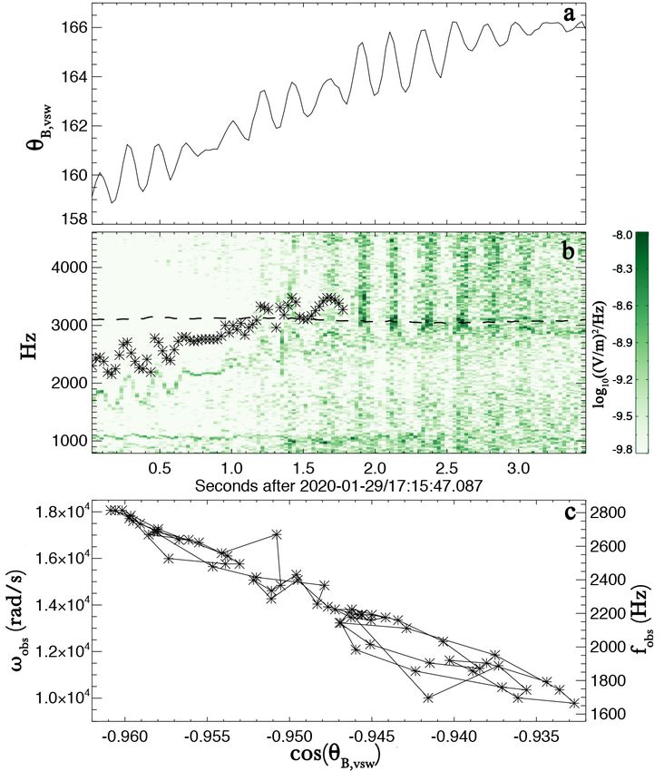
A&A 650, A97 (2021)

Fig. 3. Initial Doppler analysis for burst data recorded near June 6, 2020,
12:09:54 UTC. Panel a: angle between the ambient magnetic field vec-           Fig. 4. Same format as Fig. 3, but for a burst event recorded near January
tor (B) and the proton flow vector (V sw ). Panel b: electric field spectro-   29, 2020, 17:15:47 UTC. For this event, the frequency peak symbols are
gram. The color scale is selected to highlight the type B wave power.          not color-coded, and they are offset upward in frequency for plotting.
Colored symbols indicate the peak type B frequency for each spectrum,
plotted with an offset from the type B spectral line so that both are vis-
ible. Orange, red, and blue symbols correspond to three distinct slopes
observed in panel c. The dashed black line indicates the local electron        wave frequency should also fluctuate. Furthermore, if the stated
cyclotron frequency. Panel c: observed type B wave frequency (radi-
                                                                               assumptions hold, then a linear fit to ωobs vs. cos(θk,Vsw ) yields
ans/s) as a function of the cosine of the angle shown in panel a.
                                                                               an offset corresponding to the plasma frame frequency (ωplasma )
                                                                               and a slope corresponding to |k||Vsw |. If the angle between k and
color scheme to emphasize the type B and C wave-power peaks.                   B is known, a linear fit can be determined.
The type B spectral peak for each of the 8192 sample spectra is                    While the burst examined so far is consistent with a Doppler
indicated using asterisks, shifted down by ∼200 Hz so that both                shift as the origin of the frequency variation, the second exam-
the narrow type B peak and the symbols can be shown. Gaps                      ple shown in Fig. 4 demonstrates the effect more clearly. Figure 4
indicate times when the signal-to-noise ratio of the type B peak               has a nearly identical format to Fig. 3 for an event recorded near
fell below 10. The symbols corresponding to different times are                January 29, 2020, 17:15:47 UTC. In Fig. 4b the symbols indicat-
colored differently. Figure 3c plots the type B observed peak                  ing the identified spectral peaks are shifted upward by 600 Hz so
frequency (in radians/s, ωobs ) as a function of cos(θB,Vsw ). The             that the type B spectral line is visible. Type B spectral peaks
colors match those in Fig. 3b, and at least three intervals with               cannot be clearly separated from other wave power near fce after
distinctly different slopes are visible.                                       ∼1.7 s into the event. At this time, a coherent low-frequency ion
     Given the lack of significant magnetic field structure during             scale wave was present, causing perturbations in θB,Vsw . The cor-
this event (Figs. 1b, 3a), and the lack of observational evidence              responding frequency variation of ωobs is striking, and the fit to
for a significant electron flow during the event under study, we               the data in ωobs − cos(θB,Vsw ) space is linear.
conclude that any Doppler shift of wave frequencies must be due
to a combination of solar wind flow speed and spacecraft motion.               3.1.1. Type B Doppler-shift fitting
The wave frequency variation due to Doppler shift is given by
ωobs = ωplasma + |k||Vsw | cos(θk,Vsw ), where ωobs is the observed            Returning to the data shown in Fig. 3, estimates of |k| and ωplasma
wave frequency, |k| is the magnitude of the wave vector, |Vsw | is             can be made using the frequencies indicated in Fig. 3a and the
the solar wind speed in the frame of the spacecraft, ωplasma is the            following procedure: B and V sw vectors are used to construct
proton-frame wave frequency, and θk,Vsw is the angle between the               an orthonormal coordinate basis defined by (B × V sw ) × B,
wave vector and the plasma flow in the frame of the spacecraft.                B × V sw , and B. In this coordinate basis, the magnetic field
When ωplasma , |k|, and |Vsw | are stable over the ∼3.5 s observation          vector is B = [0, 0, 1] and the solar wind velocity vector is
time, any change in ωobs should be due to variation in cos(θk,Vsw ).           usw = [0.31, 0, −0.95]. A range of possible unit vectors k̂ are
Furthermore, if k is approximately fixed with respect to B over                defined using the polar angle θ and azimuthal angle φ. Each
this burst interval, then ωplasma should vary linearly with θB,Vsw .           angle pair (θ, φ) defines a direction of k̂ with respect to B
That is, as the ambient magnetic field direction fluctuates, the               in each spectral window, such that k(BxVsw)xB = sin(θ) cos(φ),
A97, page 4 of 10
D. M. Malaspina et al.: Electron Bernstein waves and narrowband plasma waves

Fig. 5. Doppler analysis output for the data points colored blue in Fig. 3.   Fig. 6. Doppler analysis output for the red data points in Fig. 3. Same
Panel a: wave frequency, normalized to fce , and panel b: wave number,        format as Fig. 5. Solutions with | f | > fce are not plotted.
in 1/m, both as a function of the angles θ and φ as defined in the text.
Solutions with | f | > fce are not plotted.
                                                                              reversal in polarization between the plasma frame and the space-
k(BxVsw) = sin(θ) sin(φ), and k(B) = cos(θ). With these angle                 craft frame.
definitions, the solar wind vector corresponds to [θ, φ] =                          For the range of fplasma considered, the wave vector k is
[161.8◦ , 0◦ ]. These angles are defined such that θ = 0 (θ = 180)            oblique, with 50◦ < θ < 130◦ . Given the Debye length (∼1.9 m)
points parallel (antiparallel) to B, and φ = +90 points along                 and electron gyroradius (∼97 m), lower values of |k| are more
+B × V sw .                                                                   physically reasonable: |k| = 0.15(1/m) corresponds to a wave-
     Given a k̂(θ, φ) and the measured Vsw , the quantity cos(θk,Vsw )        length of λ ≈ 42 m. Requiring lower values of |k| place k within
can then be determined. The Doppler-shift equation (ωobs =                    ∼30◦ of perpendicular to the plane defined by B and V sw . If
ωplasma + |k||Vsw | cos(θk,Vsw )) can be written as a simple linear            fplasma remains close to fce (small Doppler shift), then the wave
equation y = b + mx. Here, y is the type B ωobs in each spectral              is even more oblique (θ closer to 90◦ ).
window. A least absolute deviation linear fit to the plot of y ver-                 Figure 6 shows a similar fit output to Fig. 5, but for the earlier
sus x yields a slope (m = |k||Vsw |) and an intercept (b = ωplasma ).         part of the wave in Fig. 3a (indicated by red symbols). For these
By sweeping through all possible directions of k̂, performing                 data, the wave vector k is most oblique for fplasma far from fce ,
such a linear fit for each one, values of ωplasma and |k| can be              and slightly less oblique for fplasma near fce . The fit output values
determined throughout the (θ, φ) space.                                       of |k| are similar to those determined in Fig. 5, but slightly higher.
     Figure 5 shows the ranges of ωplasma and |k| that result from            The fit outputs from Figs. 5 and 6 overlap in the region of (θ, φ)
applying this procedure to the later part of the wave in Fig. 3a              space where fplasma ≈ fce .
(indicated by blue symbols). In Fig. 5, regions of (θ, φ) space                     We can now make another assumption: that the waves from
that yield ωplasma > ωce were removed from consideration. The                 the earlier and later parts of the burst have similar plasma-frame
fit output for fplasma / fce is shown in Fig. 5a and the fit output for       frequency ( fplasma ). If this is true, then the true k̂ is localized in
|k| is shown in Fig. 5b.                                                      the (θ, φ) region where Figs. 5 and 6 overlap, that is, along the
     Type B wave frequencies, in the spacecraft frame, are not                dark blue region of Figs. 5a and 6a. Combined with the estimate
observed to exceed the local fce in this wave event or any of                 that lower values of |k| are more physically reasonable, the fol-
the others examined thus far. If the plasma frame frequency                   lowing properties are now determined for the type B wave: (i)
is near fce , then this asymptotic behavior can be understood                 the wavelength is 21 < λ < 42 m, given 0.15 < |k| < 0.3 1/m, (ii)
as indicating times when the Doppler shift becomes small. If                  the wave vector is oblique, such that k̂ is ∼70◦ from B, (iii) k̂ is
the plasma frame frequency is much greater than fce , then the                ∼60◦ from the plane defined by B and V sw , and (iv) the plasma
observed asymptotic behavior would require a Doppler-shift sign               frame frequency ( fplasma ) is within ∼20% of the local fce . These
and magnitude that always produces f ≤ fce in the spacecraft                  are specific wave properties that can be useful to identify the
frame. Given the natural variation of usw and k between wave                  wave mode.
event observations, this is unlikely. Therefore we exclude solu-
tions with f > fce .                                                          3.1.2. Type B resonant velocities
     Negative frequency solutions are also excluded. A neg-
ative plasma frame frequency corresponds to a polarization                    The wave properties estimated above can be used to estimate the
change between the spacecraft frame (positive frequency) and                  portion of the electron distribution function with which the type
the plasma frame. However, the observed Doppler shifts are                    B waves resonate. In the case of Landau resonance, the resonant
small relative to a wave with a plasma frame frequency near fce               portion of the distribution can be determined using ωplasma = u· k.
(considering again that the observed type B frequencies asymp-                The component of the Landau resonance parallel to B satisfies
tote to f = fce ). Such small Doppler shifts are inconsistent with            v|| = ωplasma /( |k| cos(θk,B ) ). The analysis in the prior section
                                                                                                                                   A97, page 5 of 10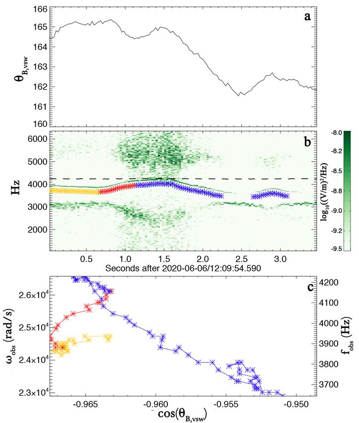
A&A 650, A97 (2021)

concluded that ωplasma ≈ ωce and k̂ ≈ 20◦ from perpendicular
to B, therefore cos(θk,B ) ≈ cos(70◦ ) ≈ 0.17. Using these values
and 0.15 < |k| < 0.3 (1/m) results in resonant velocities
that correspond to electron energies (E) of 0.19 eV < E|| <
0.75 eV. The component of the Landau resonance perpendicular
to B satisfies v⊥ = ωplasma /( |k| sin(θk,B ) ) and results in resonant
energies of 0.025 eV < E⊥ < 0.10 eV. In either case, these
resonant energies are low, near the center of the core electron
velocity distribution function.
     In the case of cyclotron resonance, the resonant portion of the
distribution can be determined using ωplasma = u·k+Nωce , where
N is a positive or negative integer and ωce = 2π fce . Cyclotron
resonant velocities satisfy u|| = (ωplasma − Nωce )/(|k| cos(θk,B )).
Because ωplasma ≈ ωce and the goal is to obtain approximate
resonant energies, the assumption ωplasma = 0.98 ωce is used
here, but is only important for the N = ±1 cyclotron resonances.
Using all other assumptions from the Landau case, the N = 1
cyclotron resonance produces 0.00007 eV < E|| < 0.0003 eV,
and N = −1 produces 0.74 eV < E|| < 3.0 eV. Extending to
N = ±2 results in 0.2 eV < E|| < 0.8 eV and 1.7 eV < E|| <
6.7 eV for positive and negative cases, respectively. All resonant
                                                                          Fig. 7. Doppler analysis output for the type C frequency peaks after the
energies listed here are in the plasma frame.                             most intense cyclotron power. Same format as Fig. 5. Solutions outside
     The −N resonances correspond to electron energies further            the range 0.45 fce < | f | < 0.8 fce are not plotted.
away from the center of the electron core distribution, which
may be more realistic for these waves given the ∼38 eV elec-
tron core temperature. In this formulation, negative values of
N correspond to the anomalous cyclotron resonance. With the               frequency occurs. Moreover, type C waves are not as narrow-
anomalous cyclotron resonance, the resonant electron guiding              band as type B waves, producing additional frequency scatter
center velocities are parallel to a component of the wave vec-            that makes fits to the ωobs vs. cos(θk,Vsw ) data more uncertain.
tor. For this case specifically, B points within ∼20◦ of sunward,             Figure 7 has the same format as Fig. 6, but shows results
and the Doppler shift is such that type B wave frequencies drop,          for type C frequency peaks from the second part of the burst
so the type B wave vector generally points along B (sunward,              event (after the most intense cyclotron power). Following similar
against the solar wind flow). Therefore the resonant electrons            reasoning to the type B analysis, the following properties are
guiding center velocities are likely sunward, implying that type          determined for the type C wave: (i) 0.08 < |k| < 0.15 1/m, (ii) a
B waves are resonant with a portion of the sunward core electron          wave vector with k̂ ≈ 5◦ from perpendicular to B, (iii) k̂ less than
distribution.                                                             ∼30◦ from perpendicular to the plane defined by B and V sw , and
                                                                          (iv) a plasma frame frequency ( fplasma ) within ∼20% of fce /2.
                                                                              Considering Landau resonance for type C waves, using
3.2. Type C: Moderately narrowband fce /2 waves
                                                                          cos(θk,B ) ≈ cos(85◦ ) and 0.08 < |k| < 0.15 (1/m), we find
The type C waves shown in Fig. 2c are moderately narrowband,              that 3 eV < E|| < 10 eV and 0.02 eV < E⊥ < 0.08 eV. With
with a bandwidth of δ f / f ≈ 12%. These waves vary in fre-               cyclotron resonance, these values produce 0.80 eV < E|| <
quency with time across the burst, but do not fall below fce /2.          2.9 eV for N = 1, and 6.5 eV < E|| < 23.0 eV for N = −1.
Similar to the type B waves, the type C frequency variation               For type C waves, as was determined for type B waves, all esti-
scales approximately linearly with variation in θB,Vsw . Strikingly,      mated resonant energies are low, near the center of the electron
the frequency variation of type C waves mirrors that of type              core distribution. Again, all resonant energies discussed are in
B waves (Fig. 2). Where type B waves decrease in frequency,               the plasma frame.
type C increase, and vice versa. When type B waves asymp-
tote to fce , type C waves simultaneously asymptote to fce /2.
                                                                          3.3. Type B and C polarization
The mirrored Doppler shift suggests that the component of the
wave vector along the solar wind direction for these two wave             Polarization is another useful piece of information to help iden-
types is oppositely directed. The type B wave vector appears to           tify wave modes. Polarization determination in this case is some-
have a component toward the Sun (Doppler frequency decrease),             what hampered by having only two reliable electric field mea-
while the type C wave vector has a component away from the                surement directions (in the plane of the heat shield), but much
Sun (Doppler frequency increase). This mirrored Doppler shift             can still be determined.
behavior is consistently observed in all of the six burst data                 Figure 8a shows the wave power spectrogram of the burst
events examined in detail where both type B and C waves are               under study. Horizontal dashed lines indicate fce and fce /2. The
distinct (other events are not shown here). A statistical study           vertical solid lines indicate the central region in which the type
is required to explore this behavior more generally, but that is          A wave power maximizes. Figures 8b and c show the results
beyond the scope of the present work.                                     of a cross-spectral analysis conducted on the two electric field
    The same Doppler-shift fitting analysis that was applied to           signals shown in Fig. 1e. These signals are orthogonal because
the type B waves can be applied to the type C waves, but with             they are rotated into spacecraft coordinates. A filter was applied
additional uncertainty in the results because the spectral peak           such that any cross-spectral result spectral bin with a wave power
frequency of the type C waves is not sufficiently distinct near           below 2 × 10⁻¹⁰ (V/m)2 /Hz is not plotted. This was done to iso-
the central region of this event, where the strongest variation in        late the type A, B, and C waves. The cross-spectral analysis was
A97, page 6 of 10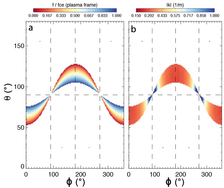
D. M. Malaspina et al.: Electron Bernstein waves and narrowband plasma waves

                                                                               4. Discussion

                                                                               From the above analysis, type B waves have the following prop-
                                                                               erties: (i) a plasma-frame frequency near fce , (ii) right-hand ellip-
                                                                               tical polarization, (iii) a wave vector magnitude of 0.15 < |k| <
                                                                               0.3 1/m, (iv) a wave vector direction ∼20◦ from perpendicular to
                                                                               B with a sunward component on either side of the central region,
                                                                               (v) resonance with low-energy electrons, close to the center of
                                                                               the electron core distribution, possibly anomalous cyclotron res-
                                                                               onance, and (vi) a frequency variation (presumed due to Doppler
                                                                               shift) that mirrors that of the type C waves.
                                                                                    Type C waves have the following properties: (i) a plasma-
                                                                               frame frequency near fce /2, (ii) left-hand elliptical polarization,
                                                                               (iii) a wave vector magnitude of 0.08 < |k| < 0.15 1/m, (iv)
                                                                               a wave vector direction ∼ 5◦ from perpendicular to B with an
                                                                               anti-sunward component on either side of the central region, (v)
                                                                               resonance with low-energy electrons, close to the center of the
                                                                               electron core distribution, possibly anomalous cyclotron reso-
                                                                               nance, and (vi) a frequency variation (presumed due to Doppler
                                                                               shift) that mirrors that of the type B waves.
                                                                                    Given these properties as well as the amplitude variation of
                                                                               type A (electron Bernstein) waves throughout the burst event, we
                                                                               conclude that the central region is likely the source region for all
                                                                               three types of wave. This conclusion is based on the observation
                                                                               that type A (electron Bernstein) wave power maximizes in this
                                                                               region, and the observation that type B and C wave frequencies
                                                                               asymptote to ∼ fce and ∼ fce /2 in this region. If this is a source
Fig. 8. Type B and C cross-spectral analysis. Panel a: electric field spec-    region, then waves will generally radiate away from it. We need
trogram near fce . Dashed horizontal lines indicate fce and fce /2. Panel b:
                                                                               to reconcile this concept with the observation that the Doppler
degree of polarization spectrum from cross-spectral analysis. Panel c:
wave ellipticity spectrum from cross-spectral analysis. Vertical lines         shift for both type B and C waves has the same sense (down
indicate the region of strongest type A wave power.                            for type B, up for type C) on either side of the source region,
                                                                               however. The source region is assumed to be a cylinder. This
                                                                               assumption is based on the gyrotropic nature of electrons in the
                                                                               ambient solar wind, combined with the observed lack of mag-
conducted in the plane of the heat shield because only these two               netic field structure at the time when the type A wave power
signals are well calibrated for this event.                                    maximizes (less than 1 degree variation of the magnetic field
    Figure 8b shows a spectrogram of degree of polarization. All               vector, see Fig. 3a).
three wave types show a high degree of polarization, indicating                     If the source region is cylindrical and elongated along B,
strong coherence between the two input signals. Figure 8c shows                then the combined solar wind and spacecraft velocity cause the
a spectrogram of the wave ellipticity, defined as the ratio of the             structure to pass over the spacecraft at a small angle relative to
minor axis to the major axis for the ellipse transcribed in the                the source region long axis. If the type B wave vectors are tilted
plane of the heat shield by the signal in each spectral bin. Red               everywhere along B (in a cone opening generally sunward), then
corresponds to right-handed polarization, and blue to left-handed              the sign of the k · V sw Doppler-shift term on either side of the
polarization. The maximum magnitude of calculated polariza-                    source region would be negative, consistent with Fig. 2b. Simi-
tion is ∼0.7, indicating elliptical polarization in the plane of the           larly, if the type C wave vectors are tilted everywhere against B
heat shield.                                                                   (in a cone opening generally anti-sunward), then the sign of the
    Figure 8c shows that type A waves are right-hand polarized,                k · V sw Doppler-shift term on either side of the source region
consistent with the interpretation that these are electron Bern-               would be positive, also consistent with Fig. 2b. Furthermore,
stein waves. Outside the central region, the type A polarization               if the type A (electron Bernstein) wave vectors were close to
is mixed and difficult to determine given the relatively low wave              perpendicular with B, but radially outward from the cylindri-
power in these signals. Type B waves are right-hand polarized                  cal source region, then the type A frequency would be slightly
outside the central region, and type C waves are left-hand polar-              higher at the start of the event and slightly lower at the end of
ized outside of the central region. Within the central region,                 the event. There is an indication of this behavior in Fig. 2b, com-
type B and C signals become more ambiguous. Type B and C                       paring the frequencies of type A wave power near 0.5 s (∼1.3 fce )
wave frequencies go to fce and fce /2, respectively, in the central            and near 3 s (∼1.15 fce ). The schematic cartoon in Fig. 9 sum-
region. The degree of polarization falls for type B waves, and the             marizes this source region concept. Here, the cones indicate the
ellipticity becomes scattered, at times appearing left-hand polar-             relative wave vector direction for each type of wave, but all types
ized. This is difficult to interpret physically, as the type A and             of wave are meant to originate from points along the full length
B signals become mixed during this interval. The type C polar-                 of the source region cylinder.
ization changes to right-handed within the central region, as the                   The estimated wavenumber ranges and orientations for
wave power becomes much more diffuse in frequency, and no                      type B and C waves allow estimates of plasma-frame wave-
distinct spectral peak is observed. This too is difficult to inter-            lengths. For type B, 61 < λ|| < 122 m, and 22 < λ⊥ < 45 m.
pret physically, as the type C signals become mixed with other                 For type C, 480 < λ|| < 901 m, and 42 < λ⊥ < 79 m. All of
wave powers present during this interval near fce /2.                          these estimated wavelengths are one to two orders of magnitude

                                                                                                                                   A97, page 7 of 10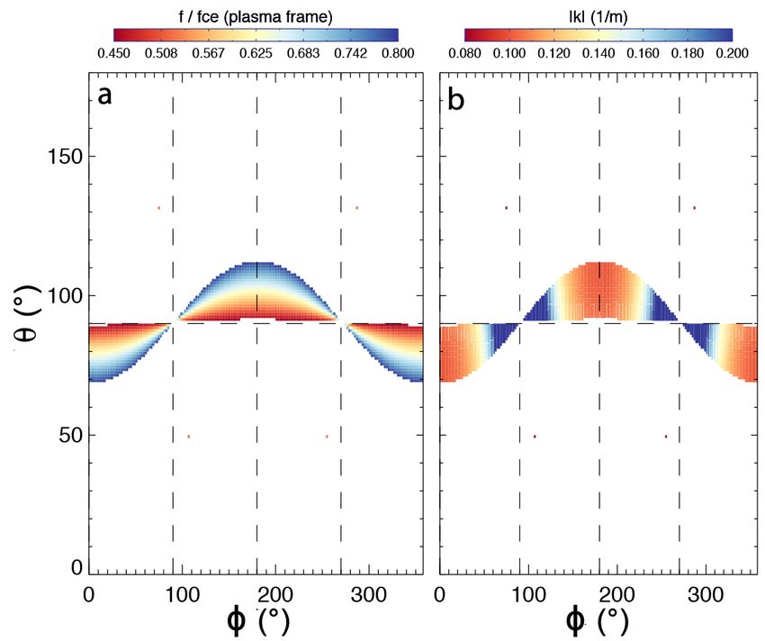
A&A 650, A97 (2021)

                                                                        cos(θk,vsw ) is not completely arbitrary, as the waves under study
                                                                        only appear when usw is within ∼20◦ of parallel to radially out-
                                                                        ward from the Sun (Malaspina et al. 2020).
                                                                             This leaves the possibility that |k| may be smaller inside the
                                                                        source region than outside. This could reduce the Doppler shift
                                                                        in the source region, and bring the wave frequency closer to its
                                                                        plasma frame value. There is some observational support for this.
                                                                        The blue points in Fig. 3c show a small cluster of points in the
                                                                        upper left corner, where the slope of the best-fit line would be
                                                                        shallower than the slope of the best-fit line to the majority of
                                                                        the blue points. This cluster of points exactly corresponds to the
                                                                        points in the center of the source region. A linear fit to these
Fig. 9. Cartoon schematic of the observed near- fce source region.      points alone for any value of θ, φ produces a slope, and therefore
                                                                        |k|, which is smaller by ∼40% than the |k| determined using the
                                                                        rest of the blue points. However, only this one event has been
                                                                        examined to this level of detail, and we do not yet know if a
longer than the Debye length (λD ∼ 1.9 m). The perpendicular            smaller |k| in the source region is a consistent property of these
wavelengths are similar to fractions of the electron gyroradius         waves.
(ρe ∼ 97 m) such that for type B 1/4ρe < λ⊥ < 1/2ρe , and for                A second change in the wave spectra also occurs in the strong
type C 1/2ρe < λ⊥ < 1ρe .                                               emission (source) regions: The wave bandwidth increases. This
     Both type B and C parallel wavelengths are significantly           behavior can be seen in Fig. 2c near 1.3 s and is observed for
smaller than the lower bound source region extent along B. This         type A, B, and C waves. The waves created in the region should
is a necessary condition for wave growth in this region. The            produce a distribution of wave vectors within the source region
source region is observed for ∼1 s. Assuming that it is embed-          that is more isotropic with respect to the background magnetic
ded in the solar wind flow, it is moving ∼250 km s−1 radially           field direction compared to the distribution of wave vectors out-
away from the Sun in the frame of the spacecraft. Assuming that         side of the source region. The more isotropic the distribution of
it extends along B and accounting for the 163◦ angle between            wave vectors, the broader the wave bandwidth should be because
B and V sw , the lower bound source region extent along B is            each wave vector produces a slightly different Doppler shift. This
∼260 km. This is much larger than the estimated parallel wave-          is consistent with the observations. A broader study is required
lengths.                                                                to determine if these are general behaviors of the wave types
     A comparison of the observations and the source region pic-        studied here.
ture presented above shows at least one unresolved discrepancy.              The instability or instabilities driving the observed waves
If type B waves have a plasma frame frequency close to fce and          are not definitively determined in this analysis, but we discuss
they are resonant with electrons, then they should be right-hand        some possibilities here. The first is the electron cyclotron drift
polarized in the plasma frame. If type B waves have a sunward           instability (ECDI; e.g., Forslund et al. 1970, 1971, 1972). The
wave vector (consistent with anomalous cyclotron resonance,             free energy for the ECDI is a cross-field drift between elec-
discussed in Sect. 3.1.2), then the Doppler shift will reduce their     trons and ions, specifically, ions moving across the magnetic
observed frequency by a small amount relative to their plasma           field. Waves radiated by this instability are observed as a cou-
frame frequency. With these properties (ωplasma ≈ ωfce , sunward        pling between electron Bernstein modes and Doppler-shifted ion
k̂, small Doppler shift), type B waves should be right-hand polar-      acoustic waves. The ECDI is highly unlikely to cause the waves
ized in the spacecraft frame. This is consistent with the observed      studied here because the magnetic field fluctuations are small.
polarization in Fig. 8.                                                 Without strong magnetic field gradients such as those at colli-
     However, if type C waves have a plasma frame frequency             sionless shocks, it is not clear how a sizeable ion beam moving
close to fce /2 and they too are resonant with electrons, then          across the magnetic field relative to the core ions and electrons
they should also be right-hand polarized in the plasma frame.           moving with the solar wind might be created.
If type C waves have an anti-sunward wave vector, consistent                 It is also possible to generate cyclotron harmonics with an
with a Doppler shift up in frequency, by an amount smaller than         electron beam drifting across the magnetic field. This insta-
their plasma frame frequency, then we expect that type C waves          bility requires that a fraction of the electrons drift with the
will also be right-hand polarized in the spacecraft frame. The          E × B- and ∇ B-drifts at a magnetic field gradient (e.g., Gary
observed polarization in Fig. 8 indicates left-hand, however. This      & Sanderson 1970). Again, magnetic field fluctuations are small
discrepancy remains unresolved and likely requires a study that         during the interval examined here, so this instability is not likely
treats more than one burst event.                                       to be active.
     For both events presented here, the type B wave frequency               Another possibility for generating the observed waves is
in the spacecraft frame approaches the electron cyclotron fre-          through nonlinear wave-wave interactions. This class of pro-
quency in the source region, where the wave emission is                 cesses usually requires a pump wave to amplify or couple to
strongest. If our Doppler-shift interpretation of the wave fre-         oscillations that mode-convert to other daughter modes. Harker
quency variation in time is correct, then why should the Doppler        & Crawford (1968) showed that a pump wave could generate two
shift consistently minimize in the source region, where the k and       daughter waves in a form of a traveling wave parametric ampli-
usw vectors presumably have an arbitrary orientation from event         fication, one of which would be cyclotron harmonic waves. The
to event?                                                               daughter waves were expected to have k VTe /Ωce . 3, but our
     The physical quantities that produce Doppler shift are |vsw |,     results suggest values >10. This process requires a very uniform
|k|, and cos(θk,vsw ). Inside and outside the source region, we know    plasma and magnetic field, which is consistent with conditions
that |vsw | is steady to our ability to measure it, and cos(θk,vsw )    of the solar wind reported during prior observations of the wave
should be somewhat arbitrary from event to event. Although              modes investigated here (Malaspina et al. 2020).

A97, page 8 of 10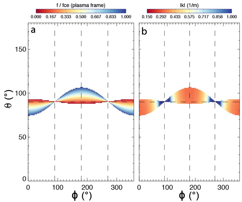
D. M. Malaspina et al.: Electron Bernstein waves and narrowband plasma waves

     A more recent study found that an electromagnetic pump            k ∼ 0.08–0.15 m−1 and the measurement of Vsw ∼ 250 km s−1 ,
wave can decay into an ion acoustic wave and electrostatic             the maximum Doppler shift possible for the type C mode is
electron Bernstein mode (e.g., Kumar & Tripathi 2006). This            only ∼3–6 kHz (i.e., assuming θkV ∼ 0◦ ). However, our esti-
study also found that the converse can occur, that is, an electro-     mates of k were derived under constraints that suggested θkV
static electron Bernstein wave in the presence of low-frequency,       could be as small as ∼50◦ . Then the Doppler-shift range for type
low-wavelength ion acoustic wave can generate electromagnetic          C waves drops to ∼2.0–3.8 kHz. The type C waves are seen at
electron cyclotron harmonics. The expected wave number for             ∼2.5–3.1 kHz in the spacecraft frame, so that their rest frame
the electron Bernstein waves is k ρce ∼ 2, while our observa-          frequencies, were the polarization to be reversed, would need to
tions suggest k ρce > 10 for the type B waves and >7 for type C        be  7, that is, a
This instability is expected to grow for 3 . k ρce,h . 15, where       wavelength well below the thermal electron gyroradius.
ρce,h is the thermal gyroradius of the hot electrons (sunward
hot electrons in our work), and higher harmonics are expected
at higher values of k ρce,h . The suprathermal electron temper-        5. Conclusions
ature is typically ∼2.5–5.0 times that of the core and total at
both 1 AU and as close as 0.17 AU (e.g., Halekas et al. 2020;          This study examined high-cadence burst data captures of elec-
Wilson et al. 2019). Using this range, we find ρce,h ∼ 146–208 m,      tric and magnetic fields of near- fce waves in the near-Sun solar
which gives us k ρce,h ∼ 22–62 for type B and ∼11–31 for type          wind. It was determined that these waves correspond to at least
C. These values are beyond the range of k ρce,h where growth           three separate, simultaneously occurring wave modes, referred
is expected. Finally, variations in the loss-cone instability have     to as types A, B, and C. Type A waves are identified as electron
been performed using a stationary (in the plasma frame) per-           Bernstein waves given the frequency distribution of their promi-
pendicular ring-beam combined with a core (e.g., Maxwellian)           nent harmonics. The modes of the type B and C waves were not
velocity distribution, but again, the expected wave numbers are        conclusively identified, but many of their properties were esti-
k ρce . 3 (e.g., Hadi et al. 2015).                                    mated, including their wave numbers (type B ∼0.23 m−1 , type C
     In the case studied here, a loss cone cannot form in the anti-    ∼0.12 1/m), wave vector direction (type B ∼70◦ , type C ∼85◦ ,
sunward direction because the hot electrons in that direction          from the ambient B-field direction), polarization (type B right-
form the strahl beam, which adiabatically narrows as these elec-       hand elliptically polarized, type C left-hand elliptically polar-
trons escape the solar corona (e.g., Berčič et al. 2020 and refer-   ized, in the frame of the spacecraft), and frequency variation. The
ences therein). However, at the studied radial distances from the      two wave types appear to be intimately connected, with opposing
sun, the strahl electron population has only just begun to scat-       frequency variation in time, but with different magnitudes (d f / f
ter into the isotropic halo (Halekas et al. 2020). It is possible      varies by ∼10% for type B waves and ∼30% for type C waves
that a loss cone can form in the sense that the sunward portion        across the studied event). Resonant electron energies were esti-
of the halo may not yet be populated (via strahl scattering) at        mated based on observed wave properties, indicating that these
these radial distances. While the SPANe instrument does have           waves grow from an instability that is active near the center of
an unobstructed field of view in the anti-sunward direction, the       the electron core population. By comparing the frequency and
angular resolution in that direction is limited, which would not       wave vector characteristics of all three waves, a source region
allow the detection of a loss cone if it was narrower than ∼20◦ .      geometry was suggested.
Furthermore, the analysis presented earlier indicates that the              While only a single wave burst was examined in detail here,
type B and C waves are resonant with electrons at much lower           the prior statistical study (Malaspina et al. 2020) demonstrated
energies than those active in a loss-cone instability as discussed     that these near- fce waves can persist for minutes to hours, occur-
here.                                                                  ring on magnetic field lines close to the theoretical Parker spiral
     Only some of the above possibilities can explain one of           geometry with low fluctuation amplitudes. These near- fce waves
the more difficult issues pertaining to these observations, the        are only observed in the near-Sun environment and become
polarizations. There are no known instabilities that would gen-        stronger and more frequently observed close to the Sun. They
erate electron-scale fluctuations in this frequency range with         preferentially occur when the electron core shows a strong sun-
a left-hand polarization. That is, none of the above instabili-        ward drift.
ties could generate an intrinsically left-hand polarized oscilla-           These properties indicate that these waves grow along field
tion with wavelengths at or below the electron gyroscale. The          lines that are most directly connected to the solar corona. They
only potential mode is the ion acoustic wave in its electromag-        therefore contain electrons that have undergone the least evolu-
netic form, but whether it can persist in this frequency range         tion since escaping the corona. Therefore the waves studied here
at these wavelengths while still being electromagnetic is not          likely play an important role in the near-Sun evolution of the
known. A possible source of ion acoustic modes is a nonlin-            solar wind electron distribution function, particularly concern-
ear wave-wave interaction, as discussed above, but these specific      ing the evolution of the cold core population as it interacts with
processes should generate the electrostatic version of the wave.       the escaping strahl electrons.
The expected wavelength of the ion acoustic mode is consistent
with the estimates for the type C waves, however. When the wave        Acknowledgements. The authors acknowledge helpful conversations with
normal angle of an ion acoustic wave is large, as estimated here       Rudolf Treumann concerning wave growth possibilities and helpful comments
for the type C waves, then the wave should be electromagnetic          from Thierry Dudok de Wit. The authors thank the Parker Solar Probe, FIELDS
                                                                       and SWEAP teams. The FIELDS experiment on Parker Solar Probe was
and not purely electrostatic.                                          designed and developed under NASA contract NNN06AA01C. All data used
     Another complication is that of Doppler shifting. The             here are publicly available on the FIELDS and SWEAP data archives: http:
left-hand polarization of the type C mode in the spacecraft            //fields.ssl.berkeley.edu/data/, http://sweap.cfa.harvard.edu/
frame is clear. The problem is that with our estimates for             pub/data/sci/sweap/.

                                                                                                                               A97, page 9 of 10
A&A 650, A97 (2021)
References Halekas, J. S., Whittlesey, P., Larson, D. E., et al. 2020, ApJS, 246, 22
Harker, K. J., & Crawford, F. W. 1968, J. App. Phys., 39, 5959
Agapitov, O. V., Dudok de Wit, T., Mozer, F. S., et al. 2020, ApJ, 891, L20 Jagarlamudi, V. K., Alexandrova, O., Berčič, L., et al. 2020, ApJ, 897, 118
Ashour-Abdalla, M., & Kennel, C. F. 1978, J. Geophys. Res., 83, 1531 Kasper, J. C., Abiad, R., Austin, G., et al. 2016, Space Sci. Rev., 204, 131
Ashour-Abdalla, M., Kennel, C. F., & Livesey, W. 1979, J. Geophys. Res., 84, Kumar, A., & Tripathi, V. K. 2006, Phys. Plasmas, 13, 052302
6540 Lacombe, C., Alexandrova, O., Matteini, L., et al. 2014, ApJ, 796, 5
Bale, S. D., Goetz, K., Harvey, P. R., et al. 2016, Space Sci. Rev., 204, 49 Li, W. Y., Graham, D. B., Khotyaintsev, Y. V., et al. 2020, Nat. Commun., 11,
Bale, S. D., Badman, S. T., Bonnell, J. W., et al. 2019, Nature, 576, 237 141
Baumgaertel, K., & Sauer, K. 1989, J. Geophys. Res., 94, 11983 Malaspina, D. M., Ergun, R. E., Bolton, M., et al. 2016, J. Geophys. Res. (Space
Berčič, L., Larson, D., Whittlesey, P., et al. 2020, ApJ, 892, 88 Phys.), 121, 5088
Bernstein, I. B. 1958, Phys. Rev., 109, 10 Malaspina, D. M., Halekas, J., Bercic, L., et al. 2020, ApJS, 246, 21
Bowen, T. A., Mallet, A., Huang, J., et al. 2020, ApJS, 246, 66 Moncuquet, M., Meyer-Vernet, N., Issautier, K., et al. 2020, ApJS, 246, 44
Breneman, A. W., Cattell, C. A., Kersten, K., et al. 2013, J. Geophys. Res. (Space Mozer, F. S., Agapitov, O. V., Bale, S. D., et al. 2020, J. Geophys. Res. (Space
Phys.), 118, 7654 Phys.), 125, e27980
Case, A. W., Kasper, J. C., Stevens, M. L., et al. 2020, ApJS, 246, 43 Pulupa, M., Bale, S. D., Bonnell, J. W., et al. 2017, J. Geophys. Res. (Space
Cattell, C., Short, B., Breneman, A., et al. 2021, A&A, 650, A8 Phys.), 122, 2836
Chaston, C. C., Bonnell, J. W., Bale, S. D., et al. 2020, ApJS, 246, 71 Stansby, D., Horbury, T. S., Chen, C. H. K., & Matteini, L. 2016, ApJ, 829, L16
Chen, C. H. K., Bale, S. D., Bonnell, J. W., et al. 2020, ApJS, 246, 53 Tong, Y., Vasko, I. Y., Artemyev, A. V., Bale, S. D., & Mozer, F. S. 2019, ApJ,
Christiansen, P., Gough, P., Martelli, G., et al. 1978, Nature, 272, 682 878, 41
Dudok de Wit, T., Krasnoselskikh, V. V., Bale, S. D., et al. 2020, ApJS, 246, 3 Verniero, J. L., Larson, D. E., Livi, R., et al. 2020, ApJS, 248, 5
Forslund, D. W., Morse, R. L., & Nielson, C. W. 1970, Phys. Rev. Lett., 25, Wilson, L. B., I, Cattell, C. A., Kellogg, P. J., et al. 2010, J. Geophys. Res. (Space
1266 Phys.), 115, A12104
Forslund, D. W., Morse, R. L., & Nielson, C. W. 1971, Phys. Rev. Lett., 27, 1424 Wilson, L. B., III, Chen, L.-J., Wang, S., et al. 2019, ApJS, 245, 24
Forslund, D., Morse, R., Nielson, C., & Fu, J. 1972, Phys. Fluids, 15, 1303 Zhang, Y., Matsumoto, H., & Kojima, H. 1998, J. Geophys. Res., 103, 20529
Fox, N. J., Velli, M. C., Bale, S. D., et al. 2016, Space Sci. Rev., 204, 7 Zhao, L. L., Zank, G. P., Adhikari, L., et al. 2020, ApJ, 898, 113
Gary, S. P., & Sanderson, J. J. 1970, J. Plasma Phys., 4, 739 Zhou, Q., Xiao, F., Yang, C., et al. 2017, Geophys. Res. Lett., 44, 5251
Hadi, F., Yoon, P. H., & Qamar, A. 2015, Phys. Plasmas, 22, 022112 Zhu, X., He, J., Verscharen, D., Duan, D., & Bale, S. D. 2020, ApJ, 901, L3
A97, page 10 of 10You can also read