Estimating Ground-Level Hourly PM2.5 Concentrations Over North China Plain with Deep Neural Networks
←
→
Page content transcription
If your browser does not render page correctly, please read the page content below
Journal of the Indian Society of Remote Sensing
https://doi.org/10.1007/s12524-021-01344-3(0123456789().,-volV)(0123456789().
                                                                         ,- volV)

    RESEARCH ARTICLE

Estimating Ground-Level Hourly PM2.5 Concentrations Over North
China Plain with Deep Neural Networks
Wenhao Zhang1,2 • Fengjie Zheng3                                                    •   Wenpeng Zhang4 • Xiufeng Yang1,2

Received: 25 August 2020 / Accepted: 9 March 2021
Ó The Author(s) 2021

Abstract
Fine particulate matter (PM2.5) has a considerable impact on the environment, climate change, and human health. Herein,
we introduce a deep neural network model for deriving ground-level, hourly PM2.5 concentrations by Himawari-8 aerosol
optical depth, meteorological variables, and land cover information. A total of 151,726 records were collected from 313
ground-level PM2.5 monitoring stations (spread across the North China Plain) to calibrate and test the proposed model. The
sample- and site-based cross-validation yielded satisfactory performance, with correlation coefficients [ 0.8 (R = 0.86 and
0.83, respectively). Furthermore, the variation in mean ground-level hourly PM2.5 concentrations, using 2017 data, showed
that the proposed method could be applied for spatiotemporal continuous PM2.5 monitoring. This study will serve as a
reference for the application of geostationary meteorological satellite to perform ground-level PM2.5 estimation and the
utilization in atmospheric monitoring.

Keywords Fine particulate matter  Deep neural networks  North China Plain  Himawari-8  Aerosol optical depth

Introduction                                                                                             monitoring sites can provide accurate PM2.5 measurements,
                                                                                                         but there are many regions for which measurements are
Fine particulate matter (PM2.5), which consists of particles                                             unavailable as there are no monitoring networks. Thus, the
with aerodynamic diameters \ 2.5 lm, has attracted con-                                                  sparse distribution of ground sites limits our capability to
siderable scientific attention (Pope & Dockery, 2006).                                                   estimate the impacts of human exposure to PM2.5, with data
Previous studies have indicated that prolonged exposure to                                               on local meteorological effects and emission sources
PM2.5 is affiliated with many human health issues including                                              absent. Consequently, it is important that models that can
respiratory problems, cardiovascular disease, cancer, and                                                accurately predict the broader spatiotemporal distribution
infectious diseases (Bartell et al., 2013; Brauer et al., 2012;                                          of ground-level PM2.5 concentrations are developed.
Chen et al., 2017; Crouse et al., 2012; Dominici et al.,                                                    Satellite has been applied to monitor ground-level PM2.5
2006; Gent et al., 2009; Guo et al., 2016; Lao et al., 2019;                                             emissions to fill in spatial gaps in ground measurement
Pope, 2000; Zhang et al., 2020). Generally, ground                                                       coverage (Chu et al., 2016; Hu et al., 2014; Kloog et al.,
                                                                                                         2012; Ma et al., 2014). Several studies were conducted for
                                                                                                         estimating PM2.5 concentrations from the aerosol optical
& Fengjie Zheng
                                                                                                         depth (AOD), derived by satellite remote sensing, includ-
  zhengfengjie84@163.com
                                                                                                         ing multiple linear regression (Chu et al., 2016; Gupta &
1
     School of Remote Sensing and Information Engineering,                                               Christopher, 2008, 2009; Kacenelenbogen et al., 2006; Liu
     North China Institute of Aerospace Engineering,                                                     et al., 2005; Paciorek et al., 2008; Schaap et al., 2009;
     Langfang 065000, China                                                                              Wang, 2003; Yao et al. 2018), mixed-effect models (Just
2
     Hebei Collaborative Innovation Center for Aerospace                                                 et al. 2015; Kloog et al. 2011, 2012, 2014; Lee et al. 2012;
     Remote Sensing Information Processing and Application,                                              Zheng et al. 2016), geographically weighted regressions
     Langfang 065000, China
3
                                                                                                         (Bai et al., 2016; Guo et al., 2017; He & Huang, 2018a, b;
     School of Space Information, Space Engineering University,                                          Hu, 2009; Ma et al., 2014; You et al., 2015; Zou et al.,
     Beijing 101416, China
4
                                                                                                         2016), and chemical transport models (Crouse et al.,
     Tianjin Earthquake Agency, Tianjin 300201, China

                                                                                                                                                           123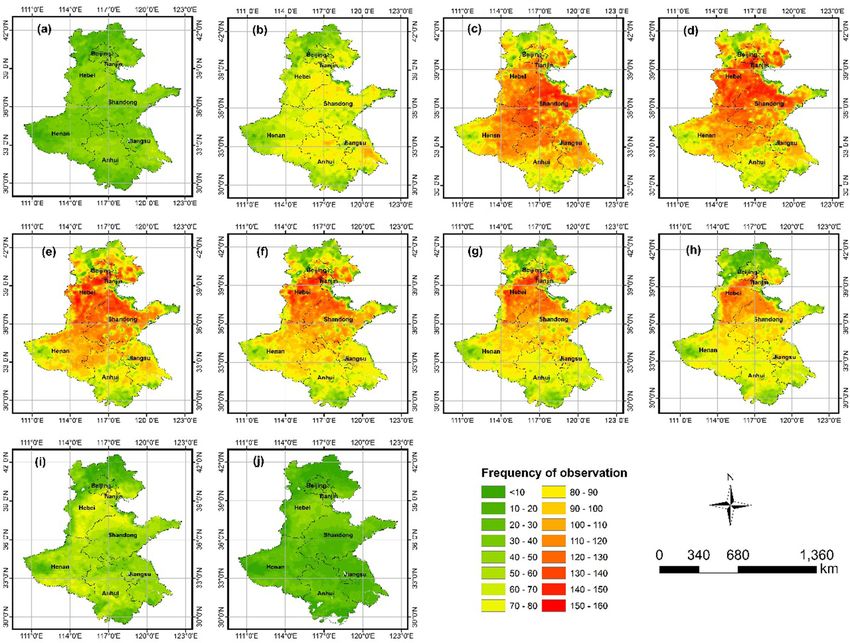
Journal of the Indian Society of Remote Sensing

2012, 2016; Hystad et al., 2012; Liu et al., 2004; van           Materials and Methods
Donkelaar et al., 2006; Wang & Chen, 2016). To improve
the model performance, an increasing number of predic-           Datasets
tors, including meteorological information, land cover, and
aerosol properties, were integrated. Thus, machine learning      Ground-Level PM2.5 Measurements
models, which are capable of complex nonlinear relation-
ships fitting, have been applied to get PM2.5 concentrations     Ground-level PM2.5 concentration dataset was obtained
from satellite observations. For example, random forests         from the China Environmental Monitoring Center
(Chen et al., 2018; Hu et al., 2017), deep belief networks       (CEMC). Hourly PM2.5 measurements from 313 air quality
(DBNs) (Li et al., 2018; Liu et al., 2018), deep neural          sites in the NCP (as shown in Fig. 1) were collated for
networks (DNNs) (Wang & Sun, 2019), and machine                  2017. These concentrations represented the hourly aver-
learning models with high-dimensional expansion (Xue             ages established at the stations by the tapered element
et al., 2019) have been used, and they have delivered            oscillating microbalance (TEOM). The accuracy of TEOM
superior prediction accuracy and applicability.                  is ± 1.5 lg/m3 (You et al., 2016). The data are available at
   All these studies were limited to the use of polar orbit      http://106.37.208.233:20035/.
satellites, however, geostationary satellites are still rarely
used in the estimation of PM2.5. These geostationary             Himawari-8 AOD
satellites are able to conduct more measurements and
facilitate the capturing of atmospheric aerosol variation        Himawari-8 was launched by the Japan Meteorological
data hourly. In particular, with the launch and operation of     Agency on October 7, 2014. It is a next-generation geo-
next-generation geostationary meteorological satellites—         stationary meteorological satellite. The AHI on board
such as the Advanced Geosynchronous Radiation Imager             Himawari-8 has 16 channels. Its spatial temporal resolution
(AGRI) on board FengYun-4A, the Advanced Himawari                is 0.5–2 km and 5–10 min, respectively (Yumimoto et al.,
Imager (AHI) on board Himawari-8/9, and the Advanced             2016; Zhang et al., 2019).
Baseline Imager (ABI) on board GOES-R—abundant AOD                  The AOD products are provided with three levels:
datasets have become available. The quality of these data        ‘‘Level2’’ (L2), ‘‘Level3’’ (L3), and ‘‘Level4’’ (L4)
has been validated: for example, it has been reported that       (Kikuchi et al., 2018). The spatial and temporal resolution
the expected uncertainty for the Himawari-8 AOD is ±             of L3 is 0.05° and 1 h, respectively. In this study, the AOD
 (0.1 ? 0.3 9 AOD) (Zhang et al., 2019), whereas the             data of L3 Version 3.0, which can be received from https://
expected uncertainty for the MODIS (C6.1) 10 km AOD              www.eorc.jaxa.jp/ptree/index.html, were collected to esti-
product is ± (0.05 ? 0.15 9 AOD) (Aldabash et al.,               mate hourly PM2.5 concentrations. It should be noted that a
2020).                                                           comprehensive AOD validation, as used in this study, can
   The North China Plain (NCP), which is renowned for            be found in our previous work (Zhang et al., 2019).
experiencing severe atmospheric pollution events, has
experienced high PM2.5 concentrations for decades owing          Meteorological and Land Cover Data
to the rapid economic and population development that has
taken place nearby. In this study, we applied the DNN            Meteorological data for 2017 were obtained from the sec-
methodology to estimate hourly ground-level PM2.5 con-           ond Modern-Era Retrospective analysis for Research and
centrations over the NCP using Himawari-8 AHI AOD                Applications (MERRA-2). It is the atmospheric product
data.                                                            supported by National Aeronautics and Space Adminis-
   The balance of this paper has been laid out as follows:       tration, with a spatial resolution of 0.5 9 0.625° (Gelaro
data sets and a detailed description of the methodology          et al., 2017; Rienecker et al., 2011). We extracted six
may be found in ‘‘Materials and Methods’’ section,               hourly meteorological factors from this dataset: surface
whereas the results and discussion have been given in            pressure (PS; as Pa), air temperature at 2 m (TMP; as K), E
‘‘Results and Discussion’’ section. The study has been           and N wind speed at 10 m above ground (EW and NW; as
concluded in ‘‘Summary and Conclusions’’ section.                m/s), relative humidity (RH; as %), and planetary boundary
                                                                 layer height (PBLH; as m). The data can be downloaded
                                                                 from the website https://disc.gsfc.nasa.gov/datasets.
                                                                    Landcover-related         variables—surface        albedo
                                                                 (ALBEDO; which is a unitless variable) and surface
                                                                 incoming shortwave flux (SWGDN; as W/m2)—were also
                                                                 extracted from the MERRA-2 data. Elevation (ELEV; as

123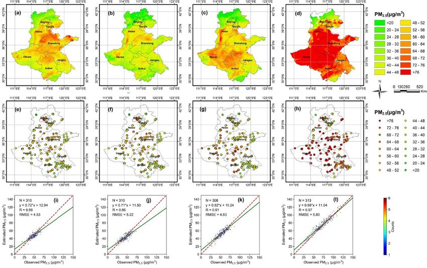
Journal of the Indian Society of Remote Sensing

Fig. 1 North China Plain elevation. Ground-level data for the study were acquired from the air quality sites (white dots) (color figure online)

m) was terrain data at 1 km, whereas the normalized dif-                  consistency. After these processes, the 11 predictors were
ference vegetation index (NDVI) was derived from                          matched with ground PM2.5 in a co-location procedure. The
MOD13A3, a monthly 1-km resolution dataset.                               predictors were collected into a station-centered pixel.
   Based on the AOD, meteorological and land cover, there                 These selection process eventually gave rise to a dataset
are 11 predictors were used to derive hourly PM2.5 con-                   consisting of 151,726 records.
centrations over the NCP. That is AOD, surface pressure,
air temperature, wind speed (E and N), PBLH, RH,                          DNN Model
ALBEDO, SWGDN, ELEV, and NDVI. Statistics for these
datasets and predictors are listed in Table 1.                            The concentrations of ground-level PM2.5 were affected by
                                                                          multiple factors, such as aerosol, meteorological, and sur-
Methods                                                                   face cover. This complex relationship is difficult to
                                                                          describe accurately with a simple linear model, and so deep
Data Integration                                                          learning, which has been widely used in fitting complex,
                                                                          nonlinear relationships, was used to estimate ground-level
Firstly, because the original data involved various coordi-               PM2.5 concentrations. Thus, a DNN model (Hinton et al.,
nate systems and spatial resolutions, all independent vari-               2012) was fitted using Eq. (1):
ables were recalibrated into the WGS84 coordinate system.                 PM2:5 ¼ f ðAOD, PS, TMP, EW, NW, PBLH, RH,
Meteorological variables and land cover data were also                       ALBEDO; SWGDN; ELEV; NDVIÞ;
recalibrated to, in this case, 0.05° resolution to ensure
                                                                                                                                           ð1Þ

                                                                                                                                   123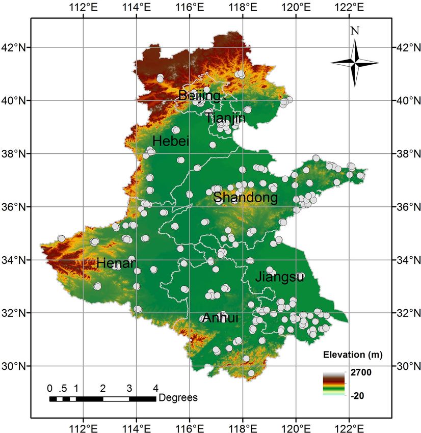
Journal of the Indian Society of Remote Sensing
Table 1 Dataset information
Datasets Predictorsa Units Spatial resolution Temporal resolution Factors
and statistics
Himawari-8 AOD – 0.05° Hourly Aerosol
MERRA-2 PS Pa 0.5 9 0.625° Hourly Meteorological
TMP K 0.5 9 0.625° Hourly Meteorological
EW m/s 0.5 9 0.625° Hourly Meteorological
NW m/s 0.5 9 0.625° Hourly Meteorological
PBLH m 0.5 9 0.625° Hourly Meteorological
RH % 0.5 9 0.625° Hourly Meteorological
ALBEDO – 0.5 9 0.625° Hourly Land cover
SWGDN W/m2 0.5 9 0.625° Hourly Land cover
GMTED2010 ELEV m 1 km – Land cover
MOD13A3 NDVI – 1 km Monthly Land cover
a
The meaning of each item is explained in text
(2) Perform DNN model fitting. To this end, all the
where f () describes the prediction function. The
151,726 records (belonging to 313 sites) were first
meaning of each predictor has been described above.
used to train the model, after which sample- and site-
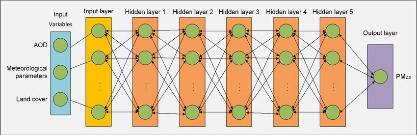
Figure 2 shows the structure of the DNN model, where
based tenfold cross-validation (CV) was carried out
it can be seen that the model contained five hidden layers
to evaluate the performance. CV was conducted as
(which contained 60, 40, 30, 20, and 10 neurons), one input
follows:
layer (which contained the 11 neurons shown in Eq. (1),
and one output layer (which consisted of PM2.5 concen- (a) For sample-based CV, the samples were
tration estimates). This gave the proposed DNN model a randomly divided into ten sets, with each set
structure of 11-60-40-30-20-10-1. It should be noted that accounting for approximately 10% of the
the numbers of layers and neurons were chosen by records. For each CV process, nine sets were
increasing the numbers of neurons until the best estimation used for training samples, with the tenth used
results were derived. to make predictions. Then, we repeated ten
Figure 3 illustrates the workflow used to estimate times until the predictions from each set were
ground-level, hourly PM2.5. The process can be described established;
as follows: (b) Site-based CV was conducted to examine
model sensitivity with respect to the number
(1) Conduct data integration, as described in ‘‘Data
of ground stations and performance with
Integration’’ section. The derived AOD, meteoro-
respect to spatial variations. The 313 sites
logical variables, and land cover, which were
were randomly split into ten sets, with each set
consistent in time and space, were treated as model
accounting for approximately 10% of the sites.
training and validation samples.
As for the sample-based CV, nine sets were
Fig. 2 Structure of the DNN model used for PM2.5 estimation
123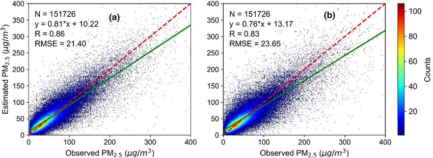
Journal of the Indian Society of Remote Sensing

Fig. 3 Workflow applied to
estimate ground-level, hourly
PM2.5 concentrations

              used to fit the model, with the tenth used to     Results and Discussion
              make predictions. PM2.5 concentration predic-
              tions were finally obtained by completing ten     Descriptive Statistics
              CV cycles;
       (c)    Finally, to evaluate the levels of agreement,     Variable histograms, covering all 151,726 samples, are
              linear fit statistics for model predictions vs    presented in Fig. 4. The surface pressure (PS) was found to
              observations were performed. The statistical      be almost exponentially distributed, whereas air tempera-
              indicators include the correlation coefficient    ture (TMP) was approximately bimodal in its distribution.
              (R), slope, y intercept, and prediction root      The E wind speed, N wind speed, PBLH, surface albedo,
              mean squared error (RMSE).                        surface incoming shortwave flux (SWGDN), RH, and
(3)    Finally, the prediction data (locations with no ground   NDVI were found to have approximately normal distribu-
       PM2.5 observations) were input into the derived          tions. The other variables, including elevation, AOD, and
       DNN model to obtain spatial distributions of hourly      PM2.5, exhibited similar logarithmic distributions. The
       PM2.5 concentrations over the NCP.                       minimum, maximum, and mean PM2.5 concentrations were
                                                                1, 534, and 55.13 lg/m3, respectively, whereas the mini-
                                                                mum, maximum, and mean AOD were calculated to be 0,
                                                                2.99, and 0.4, respectively, with the high AOD and PM2.5
                                                                maximums indicating that severe pollution was experi-
                                                                enced over the NCP. Their standard deviations were cal-
                                                                culated as 0.34 and 42.15 mg/m3, respectively, indicating

                                                                                                                 123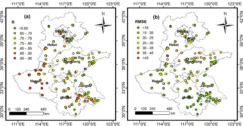
Journal of the Indian Society of Remote Sensing

Fig. 4 Descriptive statistics for dependent and independent variables (minimums, maximums, means, and standard deviations). The meaning of
each item is explained in text

that there had been significant fluctuations in the atmo-
spheric particulate matter concentrations.

Variable Importance Analysis

To evaluate the potential effect of each predictor to the
proposed DNN, we conducted a variable importance
analysis. In Fig. 5, the variables for predicting PM2.5 have
been represented in the y axis, with the percentage RMSE
increase without using the corresponding variable
(%IncRMSE) shown on the x axis. The figure shows that
AOD (55.07%) was the variable with the highest contri-
bution, which would be attributable to its strong correlation
with PM2.5 concentrations. The %IncRMSE calculated
without using air temperature as a predictor was 45.92%,
followed by PBLH (41.21%), SWGDN (35.07%), RH                          Fig. 5 Variable importance analysis. The x axis indicates the
(34.86%), N wind speed (32.09%), surface pressure                      percentage RMSE increase achieved without using the corresponding
                                                                       predictor (%IncRMSE)

123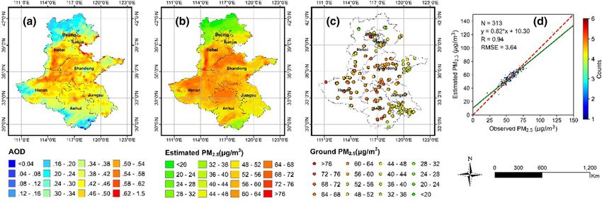
Journal of the Indian Society of Remote Sensing

(30.63%), E wind speed (24.22%), and surface albedo                     land surface variables to estimate point ground-level PM2.5
(24.01%).                                                               meant that it was difficult for meteorological parameters
   Figure 5 also shows that elevation and NDVI were the                 with relatively coarse spatial resolution (0.5° 9 0.625°) to
weakest contributing variables for hourly PM2.5 concen-                 characterize detailed spatial variations. The other reason
trations. These relatively low contributions may have been              was that a spatial average would lead to high values being
due to the small elevation variations over the NCP (shown               averaged and low values being overwhelmed. Taken
in Fig. 4j). Furthermore, hourly PM2.5 concentrations,                  together, these points meant that when we compared spa-
usually with high frequency variations, were likely to be               tially averaged estimations with ground measurements, low
less affected by variables that varied only slowly over time,           values appeared to be overestimated and high values
such as NDVI.                                                           underestimated.
                                                                            The spatial performance of the sample-based CV is
Model Performance and Validation                                        illustrated in Fig. 7, where it can be seen that both R and
                                                                        RMSE (Figs. 7a, b, respectively) exhibit spatial variations.
The scatter plot showing ground observed (x axis) and                   The R ranged between 0.48 and 0.93, whereas the RMSE
estimated (y axis) PM2.5 concentrations for sample- and                 ranged between 13.33 and 45.63, with 81% of R [ 0.75
site-based CVs is shown in Fig. 6a, b. The R, RMSE, slope,              (254 sites out of 313), and 68% of the RMSE \ 25 lg/m3
and y intercept of sample-based CVs were 0.86, 21.40 lg/                (213 out of the 313 sites). With respect to geographic
m3, 0.81, and 10.22 lg/m3, respectively; with regard to the             distribution, sites in Henan Province performed better, with
site-based CVs, the corresponding values were 0.83,                     the RMSE being lower in Anhui and Zhejiang.
23.65 lg/m3, 0.76, and 13.17 lg/m3, respectively. This                      Scatter plots for ground-observed (x axis) and estimated
good level of consistency demonstrated that the proposed                (y axis) daily and monthly PM2.5 concentrations are shown
DNN model was capable of achieving satisfactory                         in Figs. 8a, b. The daily data R and RMSE were calculated
performance.                                                            to be 0.81 and 24.94 lg/m3, whereas the corresponding
   We noted that the site-based CV outcome was compa-                   estimates for the monthly data were 0.90 and 9.91 lg/m3,
rable with that of the sample-based CV, which indicated                 respectively, showing that the model could accurately
that the proposed model had good spatial prediction                     represent seasonal PM2.5 levels, with only small deviations.
capability. In addition, both the regression linear fit slopes
were \ unity (0.81 and 0.76), which implied that the DNN                Map of PM2.5 Estimation
model tended to develop results that were slightly under-
estimated in comparison with the observed PM2.5 concen-                 The distributions of seasonal average PM2.5 over NCP in
tration. This underestimation was confirmed by noting                   2017 are shown in Fig. 9; in Fig. 9a–d; the seasonal vari-
observed PM2.5 concentrations [ 54 lg/m3.                               ations in PM2.5 are clearly observable. The highest PM2.5
   We deduced two possible reasons for the ground-ob-                   estimations were in winter, followed by spring, and then
served PM2.5 concentration underestimation by the model.                autumn, with the lowest values appearing in summer. Mean
Firstly, using spatially averaged AOD, meteorological, and              PM2.5 estimations for spring, summer, autumn, and winter

Fig. 6 Scatter plots for tenfold cross-validations (CVs): a sample-based CV; b site-based CV

                                                                                                                          123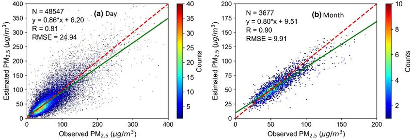
Journal of the Indian Society of Remote Sensing

Fig. 7 Cross-validation spatial performance: a R; b RMSE

Fig. 8 Model validation scatter plots: a daily data; b monthly averages

were 48.93, 39.85, 48.06, and 74.78 lg/m3, respectively.                  was complex. Meanwhile, a heavily polluted region was
The seasonal ground-level PM2.5 observations showed                       revealed at the junction of the five provinces (Hebei,
spatial distributions similar to those seen for the estimates,            Henan, Anhui, Jiangsu, and Shandong). Scatter plots for
as shown in Figs. 9e–h. The R values of four seasons were                 annualized ground-level observations vs estimated PM2.5
0.88, 0.86, 0.91, and 0.97, respectively (Figs. 9i–l),                    levels are shown in Fig. 10c, with the R and RMSE cal-
whereas the corresponding RMSEs were 4.53, 5.22, 4.83,                    culated to be 0.94 and 3.64 lg/m3 (Fig. 10d), respectively.
and 5.80 lg/m3, respectively.                                                 Annualized PM2.5 estimate averages for ten hours
   Annual estimated PM2.5 patterns for the NCP are plotted                (00:00–09:00 (Coordinated Universal Time, UTC)), in
in Fig. 10. Generally, low AOD and PM2.5 levels occurred                  2017, are shown in Fig. 11, whereas Fig. 12 shows the
in NW Hebei Province, with its low population density and                 corresponding ground-level observation frequencies. Fig-
few industries. These spatial AOD (Fig. 10a) and PM2.5                    ure 11 proves that the proposed model can provide at least
(Fig. 10b) distribution results were not completely consis-               ten hourly PM2.5 estimations in one day for any given area,
tent, however, which indicated that their interrelationship               i.e., it can provide PM2.5 concentration information at high

123
Journal of the Indian Society of Remote Sensing

Fig. 9 Spatial distributions for spring (March, April, and May),           PM2.5 concentrations: a–d estimates; e–h ground-observations; i–
summer (June, July, and August), autumn (September, October, and           l ground observation versus estimates distribution scatter plots
November), and winter (December, January, and February) mean

Fig. 10 Spatial distribution for annual average PM2.5 concentrations: a AOD; b estimates; c ground-level observations; d scatter plot for ground-
level observations versus estimates

frequencies. In Fig. 12, we can see that the spatial distri-               decreased as the solar zenith angle increased (Zhang et al.,
bution of ground-level measurements exhibited temporal                     2019).
variations, peaking at noon, local time (03:00 UTC),                          Variations in annual average hourly PM2.5 estimations
whereas the data volume gradually decreased in the                         experienced by different cities are shown in Fig. 13. The
mornings and afternoons. This could be explained by the                    cities were selected based on their distribution and repre-
fact that the ability of the satellite to capture aerosol signals          sentativeness for different regions. They displayed similar
                                                                           trends, i.e., over the period 00:00–09:00 (UTC), the PM2.5

                                                                                                                                     123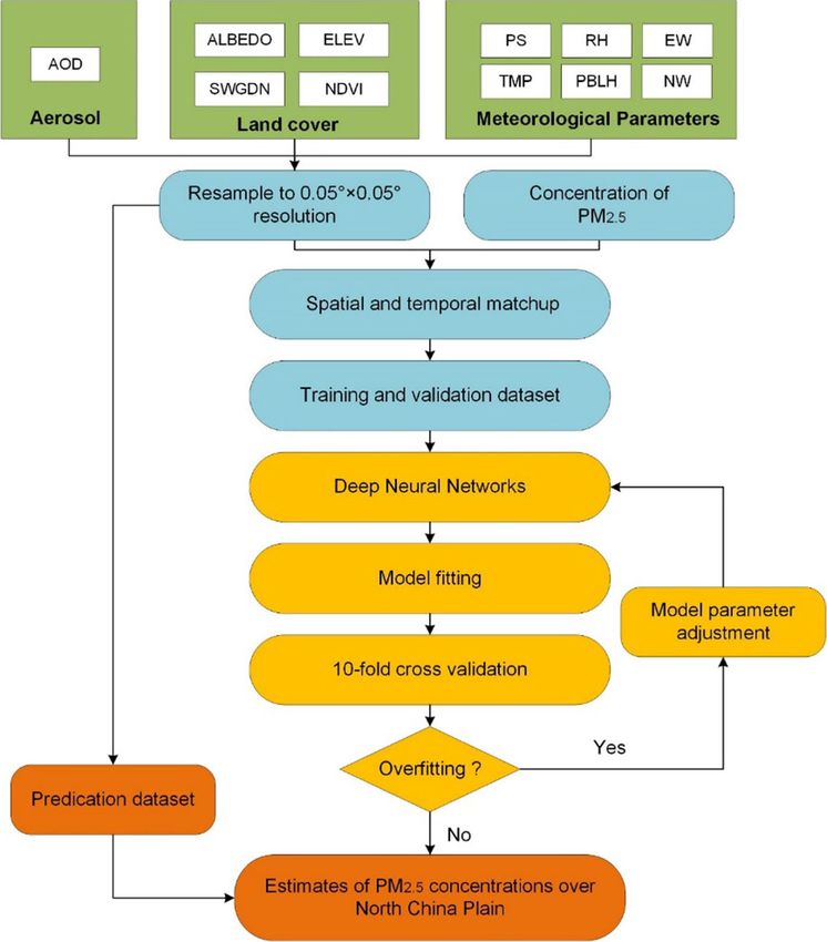
Journal of the Indian Society of Remote Sensing
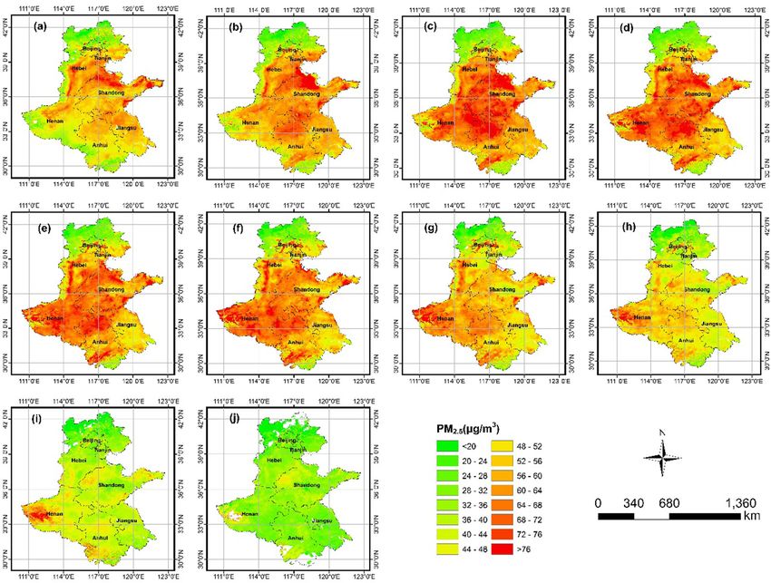
Fig. 11 Annualized PM2.5 estimate averages for different hours (as UTC) in 2017: a–j represent 00:00–09:00, respectively
levels peaked at certain times and then decreased. The using aerosol product (from a new-generation geostation-
peaks for Hefei (117.24, 31.84), Shijiazhuang (114.52, ary satellite Himawari-8), meteorological, and land cover
38.03), Nanjing (118.80, 32.07), and Jinan (117.13, 36.64) information to estimate hourly ground-level PM2.5 con-
appeared at either 02:00 or 03:00 (UTC), whereas Beijing centrations of NCP. The estimated PM2.5 concentrations
(116.41, 39.90) and Zhengzhou (113.64, 34.75) peaked at had a spatial and temporal resolution of 0.05° and 1 h,
01:00. Minimum values were experienced by all cities at respectively, which can capture detailed variations in
either 08:00 or 09:00 (UTC). Figure 13 shows that the temporal PM2.5 distributions than would have been possi-
proposed model could describe variety in PM2.5 concen- ble using polar orbit satellites such as MODIS. A total of
trations at a temporal resolution of 1 h. 11 independent variables were used to fit the proposed
model: AHI AOD, surface pressure, air temperature, E and
N wind speeds, PBLH, RH, surface albedo, SWGDN,
Summary and Conclusions elevation, and NDVI. Through data integration, a total of
151,726 records related to 313 ground stations were col-
It is still a challenge to derive high temporal ground-level lected. To validate the model performance, tenfold CV was
PM2.5 accurately using satellite-derived AOD data, espe- conducted, and it was found that both sample-based
cially for regions with higher particulate matter concen- (R = 0.86, RMSE = 21.40 lg/m3) and site-based
trations and complex compositions, such as the NCP, (R = 0.83, RMSE = 23.65 lg/m3) CVs exhibited satisfac-
which has become heavily polluted with respect to PM2.5. tory performances. R values were calculated to be 0.81 and
Herein, we presented a DNN model that was calibrated
123Journal of the Indian Society of Remote Sensing
Fig. 12 Annualized frequencies for PM2.5 concentration estimates for different hours in 2017 (as UTC): a–j represent 00:00–09:00, respectively
spring, autumn, and summer. The annual patterns showed
that low PM2.5 concentration levels occurred in NW Hebei
Province, whereas the area representing the junction of
Hebei, Henan, Anhui, Jiangsu, and Shandong provinces
was identified as being heavily polluted.
We also produced mapping, in which 2017 hourly data
were used to generate annualized averages for ten hours
(from 00:00 to 09:00 UTC). These results suggested that
the proposed model could provide at least ten different
hourly PM2.5 estimations daily, and thus, it had the capa-
bility to reveal high levels of atmosphere variation over
time. Such successful testing allowed us to conclude that
new-generation geostationary satellites have the potential
Fig. 13 Annual mean variations in 2017 for hourly PM2.5 concen- to be used as useful data sources for ground-level PM2.5
trations in selected study area cities
estimation.
0.90, respectively, for daily and monthly averaged PM2.5 Acknowledgements The authors acknowledge Himawari-8/AHI
levels. AOD support by the P-Tree System, Japan Aerospace Exploration
When mapped, the estimated PM2.5 concentrations for Agency (JAXA). MODIS data were supplied by NASA. The ground-
the NCP showed clear seasonal variations, with the highest based PM2.5 concentrations were obtained from the China Environ-
mental Monitoring Center (CEMC). The MERRA-2 data were
PM2.5 concentrations appearing in winter, followed by
123Journal of the Indian Society of Remote Sensing
supported by Goddard Earth Sciences Data and Information Services temperature in China: A multi-city study. Environment Interna-
Center (GES DISC). tional, 98, 82–88. https://doi.org/10.1016/j.envint.2016.10.004
Chu, Y., Liu, Y., Li, X., Liu, Z., Lu, H., Lu, Y., & Xiang, H. (2016). A
Funding This study was funded by National Natural Science Foun- review on predicting ground PM2.5concentration using satellite
dation of China, Grant number 41801255, Natural Science Founda- aerosol optical depth. Atmosphere, 7(10), 129. https://doi.org/10.
tion of Hebei Province, Grant number D2020409003, and Civil 3390/atmos7100129
Aerospace Pre-research Project, Grant number D040102. Science for Crouse, D. L., Peters, P. A., van Donkelaar, A., Goldberg, M. S.,
Earthquake Resilience, grant number XH19003Y. Villeneuve, P. J., Brion, O., & Burnett, R. T. (2012). Risk of
nonaccidental and cardiovascular mortality in relation to long-
Availability of Data and Material The ground PM2.5 measurements term exposure to low concentrations of fine particulate matter: A
can be obtained from http://106.37.208.233:20035/. The Himawari-8 Canadian national-level cohort study. Environmental Health
AOD can be obtained from https://www.eorc.jaxa.jp/ptree/index.html. perspectives, 120(5), 708–714. https://doi.org/10.1289/ehp.
The MERRA-2 data can be obtained from https://disc.gsfc.nasa.gov/ 1104049
datasets. Crouse, D. L., Philip, S., Van Donkelaar, A., Martin, R. V., Jessiman,
B., Peters, P. A., & Burnett, R. T. (2016). A new method to
jointly estimate the mortality risk of long-term exposure to fine
Declarations particulate matter and its components. Scientific Reports, 6(1),
1–10. https://doi.org/10.1038/srep18916
Conflicts of interest The authors declare no conflict of interest. Dominici, F., Peng, R. D., Bell, M. L., Pham, L., McDermott, A.,
Zeger, S. L., & Samet, J. M. (2006). Fine particulate air pollution
Open Access This article is licensed under a Creative Commons and hospital admission for cardiovascular and respiratory
Attribution 4.0 International License, which permits use, sharing, diseases. Journal of the American Medical Association,
adaptation, distribution and reproduction in any medium or format, as 295(10), 1127–1134. https://doi.org/10.1001/jama.295.10.1127
long as you give appropriate credit to the original author(s) and the Gelaro, R., McCarty, W., Suárez, M. J., Todling, R., Molod, A.,
source, provide a link to the Creative Commons licence, and indicate Takacs, L., & Zhao, B. (2017). The modern-era retrospective
if changes were made. The images or other third party material in this analysis for research and applications, version 2 (MERRA-2).
article are included in the article’s Creative Commons licence, unless Journal of Climate, 30(14), 5419–5454. https://doi.org/10.1175/
indicated otherwise in a credit line to the material. If material is not JCLI-D-16-0758.1
included in the article’s Creative Commons licence and your intended Gent, J. F., Koutrakis, P., Belanger, K., Triche, E., Holford, T. R.,
use is not permitted by statutory regulation or exceeds the permitted Bracken, M. B., & Leaderer, B. P. (2009). Symptoms and
use, you will need to obtain permission directly from the copyright medication use in children with asthma and traffic-related
holder. To view a copy of this licence, visit http://creativecommons. sources of fine particle pollution. Environmental Health Per-
org/licenses/by/4.0/. spectives, 117(7), 1168–1174. https://doi.org/10.1289/ehp.
0800335
Guo, Y., Tang, Q., Gong, D. Y., & Zhang, Z. (2017). Estimating
ground-level PM2.5 concentrations in Beijing using a satellite-
References based geographically and temporally weighted regression model.
Remote Sensing of Environment, 198, 140–149. https://doi.org/
Aldabash, M., Balcik, F. B., & Glantz, P. (2020). Validation of 10.1016/j.rse.2017.06.001
MODIS C6.1 and MERRA-2 AOD using AERONET observa- Guo, Y., Zeng, H., Zheng, R., Li, S., Barnett, A. G., Zhang, S., &
tions: A comparative study over Turkey. Atmosphere, 11(9), 905. Williams, G. (2016). The association between lung cancer
https://doi.org/10.3390/ATMOS11090905 incidence and ambient air pollution in China: A spatiotemporal
Bai, Y., Wu, L., Qin, K., Zhang, Y., Shen, Y., & Zhou, Y. (2016). A analysis. Environmental Research, 144, 60–65. https://doi.org/
geographically and temporally weighted regression model for 10.1016/j.envres.2015.11.004
ground-level PM2.5 estimation from satellite-derived 500 m Gupta, P., & Christopher, S. A. (2008). Seven year particulate matter
resolution AOD. Remote Sensing. https://doi.org/10.3390/ air quality assessment from surface and satellite measurements.
rs8030262 Atmospheric Chemistry and Physics, 8(12), 3311–3324. https://
Bartell, S. M., Longhurst, J., Tjoa, T., Sioutas, C., & Delfino, R. J. doi.org/10.5194/acp-8-3311-2008
(2013). Particulate air pollution, ambulatory heart rate variabil- Gupta, P., & Christopher, S. A. (2009). Particulate matter air quality
ity, and cardiac arrhythmia in retirement community residents assessment using integrated surface, satellite, and meteorological
with coronary artery disease. Environmental Health Perspec- products: Multiple regression approach. Journal of Geophysical
tives, 121(10), 1135–1141. https://doi.org/10.1289/ehp.1205914 Research Atmospheres, 114(14), D14205. https://doi.org/10.
Brauer, M., Amann, M., Burnett, R. T., Cohen, A., Dentener, F., 1029/2008JD011496
Ezzati, M., & Thurston, G. D. (2012). Exposure assessment for He, Q., & Huang, B. (2018a). Satellite-based high-resolution PM2.5
estimation of the global burden of disease attributable to outdoor estimation over the Beijing–Tianjin–Hebei region of China using
air pollution. Environmental Science and Technology, 46(2), an improved geographically and temporally weighted regression
652–660. https://doi.org/10.1021/es2025752 model. Environmental Pollution, 236, 1027–1037. https://doi.
Chen, G., Li, S., Knibbs, L. D., Hamm, N. A., Cao, W., Li, T., & Guo, org/10.1016/j.envpol.2018.01.053
Y. (2018). A machine learning method to estimate PM2.5 He, Q., & Huang, B. (2018b). Satellite-based mapping of daily high-
concentrations across China with remote sensing, meteorological resolution ground PM2.5 in China via space-time regression
and land use information. Science of the Total Environment, 636, modeling. Remote Sensing of Environment, 206, 72–83. https://
52–60. https://doi.org/10.1016/j.scitotenv.2018.04.251 doi.org/10.1016/j.rse.2017.12.018
Chen, G., Zhang, W., Li, S., Zhang, Y., Williams, G., Huxley, R., & Hinton, G., Deng, L., Yu, D., Dahl, G. E., Mohamed, A. R., Jaitly, N.,
Guo, Y. (2017). The impact of ambient fine particles on & Kingsbury, B. (2012). Deep neural networks for acoustic
influenza transmission and the modification effects of modeling in speech recognition: The shared views of four
123Journal of the Indian Society of Remote Sensing
research groups. IEEE Signal Processing Magazine, 29(6), Li, T., Shen, H., Yuan, Q., & Zhang, L. (2018). Deep learning for
82–97. https://doi.org/10.1109/MSP.2012.2205597 ground-level PM2.5 prediction from satellite remote sensing data.
Hu, X., Belle, J. H., Meng, X., Wildani, A., Waller, L. A., Strickland, International Geoscience and Remote Sensing Symposium
M. J., & Liu, Y. (2017). Estimating PM2.5 concentrations in the (IGARSS), 2018, 7581–7584. https://doi.org/10.1109/IGARSS.
conterminous united states using the random forest approach. 2018.8519036
Environmental Science and Technology, 51(12), 6936–6944. Liu, Y., Cao, G., Zhao, N., Mulligan, K., & Ye, X. (2018). Improve
https://doi.org/10.1021/acs.est.7b01210 ground-level PM2.5 concentration mapping using a random
Hu, X., Waller, L. A., Lyapustin, A., Wang, Y., Al-Hamdan, M. Z., forests-based geostatistical approach. Environmental Pollution,
Crosson, W. L., & Liu, Y. (2014). Estimating ground-level PM2.5 235, 272–282. https://doi.org/10.1016/j.envpol.2017.12.070
concentrations in the Southeastern United States using MAIAC Liu, Y., Park, R. J., Jacob, D. J., Li, Q., Kilaru, V., & Sarnat, J. A.
AOD retrievals and a two-stage model. Remote Sensing of (2004). Mapping annual mean ground-level PM2.5 concentra-
Environment, 140, 220–232. https://doi.org/10.1016/j.rse.2013. tions using Multiangle Imaging Spectroradiometer aerosol
08.032 optical thickness over the contiguous United States. Journal of
Hu, Z. (2009). Spatial analysis of MODIS aerosol optical depth, Geophysical Research D: Atmospheres, 109(22), 1–10. https://
PM2.5, and chronic coronary heart disease. International Journal doi.org/10.1029/2004JD005025
of Health Geographics, 8(1), 27. https://doi.org/10.1186/1476- Liu, Y., Sarnat, J. A., Kilaru, V., Jacob, D. J., & Koutrakis, P. (2005).
072X-8-27 Estimating ground-level PM2.5 in the eastern United States using
Hystad, P., Demers, P. A., Johnson, K. C., Brook, J., van Donkelaar, satellite remote sensing. Environmental Science and Technology,
A., Lamsal, L., & Brauer, M. (2012). Spatiotemporal air 39(9), 3269–3278. https://doi.org/10.1021/es049352m
pollution exposure assessment for a Canadian population-based Ma, Z., Hu, X., Huang, L., Bi, J., & Liu, Y. (2014). Estimating
lung cancer case-control study. Environmental Health, 11(1), ground-level PM2.5 in China using satellite remote sensing.
1–13. https://doi.org/10.1186/1476-069X-11-22 Environmental Science and Technology, 48(13), 7436–7444.
Just, A. C., Wright, R. O., Schwartz, J., Coull, B. A., Baccarelli, A. https://doi.org/10.1021/es5009399
A., Tellez-Rojo, M. M., & Kloog, I. (2015). Using high- Paciorek, C. J., Liu, Y., Moreno-Macias, H., & Kondragunta, S.
resolution satellite aerosol optical depth to estimate daily PM2.5 (2008). Spatiotemporal associations between GOES aerosol
geographical distribution in Mexico City. Environmental Science optical depth retrievals and ground-level PM2.5. Environmental
and Technology, 49(14), 8576–8584. https://doi.org/10.1021/acs. Science and Technology, 42(15), 5800–5806. https://doi.org/10.
est.5b00859 1021/es703181j
Kacenelenbogen, M., Léon, J. F., Chiapello, I., & Tanré, D. (2006). Pope, C. A. (2000). Epidemiology of fine particulate air pollution and
Characterization of aerosol pollution events in France using human health: Biologic mechanisms and who’s at risk?
ground-based and POLDER-2 satellite data. Atmospheric Chem- Environmental Health Perspectives, 108(SUPPL. 4), 713–723.
istry and Physics, 6(12), 4843–4849. https://doi.org/10.5194/ https://doi.org/10.2307/3454408
acp-6-4843-2006 Pope, C. A., & Dockery, D. W. (2006). Health effects of fine
Kikuchi, M., Murakami, H., Suzuki, K., Nagao, T. M., & Higurashi, particulate air pollution: Lines that connect. Journal of the Air
A. (2018). Improved hourly estimates of aerosol optical thick- and Waste Management Association, 56(6), 709–742. https://doi.
ness using spatiotemporal variability derived from Himawari-8 org/10.1080/10473289.2006.10464485
geostationary satellite. IEEE Transactions on Geoscience and Rienecker, M. M., Suarez, M. J., Gelaro, R., Todling, R., Bacmeister,
Remote Sensing, 56(6), 3442–3455. https://doi.org/10.1109/ J., Liu, E., & Woollen, J. (2011). MERRA: NASA’s modern-era
TGRS.2018.2800060 retrospective analysis for research and applications. Journal of
Kloog, I., Chudnovsky, A. A., Just, A. C., Nordio, F., Koutrakis, P., climate, 24(14), 3624–3648. https://doi.org/10.1175/JCLI-D-11-
Coull, B. A., & Schwartz, J. (2014). A new hybrid spatio- 00015.1
temporal model for estimating daily multi-year PM2.5 concen- Schaap, M., Apituley, A., Timmermans, R. M. A., Koelemeijer, R.
trations across northeastern USA using high resolution aerosol B. A., & De Leeuw, G. (2009). Exploring the relation between
optical depth data. Atmospheric Environment, 95, 581–590. aerosol optical depth and PM2.5 at Cabauw, the Netherlands.
https://doi.org/10.1016/j.atmosenv.2014.07.014 Atmospheric Chemistry and Physics, 9(3), 909–925. https://doi.
Kloog, I., Koutrakis, P., Coull, B. A., Lee, H. J., & Schwartz, J. org/10.5194/acp-9-909-2009
(2011). Assessing temporally and spatially resolved PM2.5 van Donkelaar, A., Martin, R. V., & Park, R. J. (2006). Estimating
exposures for epidemiological studies using satellite aerosol ground-level PM2.5 using aerosol optical depth determined from
optical depth measurements. Atmospheric Environment, 45(35), satellite remote sensing. Journal of Geophysical Research
6267–6275. https://doi.org/10.1016/j.atmosenv.2011.08.066 Atmospheres, 111(21), D21201. https://doi.org/10.1029/
Kloog, I., Nordio, F., Coull, B. A., & Schwartz, J. (2012). 2005JD006996
Incorporating local land use regression and satellite aerosol Wang, B., & Chen, Z. (2016). High-resolution satellite-based analysis
optical depth in a hybrid model of spatiotemporal PM2.5 of ground-level PM2.5 for the city of Montreal. Science of the
exposures in the mid-atlantic states. Environmental Science Total Environment, 541, 1059–1069. https://doi.org/10.1016/j.
and Technology, 46(21), 11913–11921. https://doi.org/10.1021/ scitotenv.2015.10.024
es302673e Wang, J. (2003). Intercomparison between satellite-derived aerosol
Lao, X. Q., Guo, C., Chang, L. Y., Bo, Y., Zhang, Z., Chuang, Y. C., optical thickness and PM2.5 mass: Implications for air quality
& Chan, T. C. (2019). Long-term exposure to ambient fine studies. Geophysical Research Letters, 30(21), 2095. https://doi.
particulate matter (PM2.5) and incident type 2 diabetes: A org/10.1029/2003GL018174
longitudinal cohort study. Diabetologia, 62(5), 759–769. https:// Wang, X., & Sun, W. (2019). Meteorological parameters and gaseous
doi.org/10.1007/s00125-019-4825-1 pollutant concentrations as predictors of daily continuous PM2.5
Lee, H. J., Coull, B. A., Bell, M. L., & Koutrakis, P. (2012). Use of concentrations using deep neural network in Beijing–Tianjin–
satellite-based aerosol optical depth and spatial clustering to Hebei. China. Atmospheric Environment, 211, 128–137. https://
predict ambient PM2.5 concentrations. Environmental Research, doi.org/10.1016/j.atmosenv.2019.05.004
118, 8–15. https://doi.org/10.1016/j.envres.2012.06.011 Xue, T., Zheng, Y., Tong, D., Zheng, B., Li, X., Zhu, T., & Zhang, Q.
(2019). Spatiotemporal continuous estimates of PM2.5
123Journal of the Indian Society of Remote Sensing
concentrations in China, 2000–2016: A machine learning Zhang, L., Wilson, J. P., MacDonald, B., Zhang, W., & Yu, T. (2020).
method with inputs from satellites, chemical transport model, The changing PM2.5 dynamics of global megacities based on
and ground observations. Environment International, 123, long-term remotely sensed observations. Environment Interna-
345–357. https://doi.org/10.1016/j.envint.2018.11.075 tional, 142, 105862. https://doi.org/10.1016/j.envint.2020.
Yao, F., Si, M., Li, W., & Wu, J. (2018). A multidimensional 105862
comparison between MODIS and VIIRS AOD in estimating Zhang, W., Xu, H., & Zhang, L. (2019). Assessment of Himawari-8
ground-level PM2.5 concentrations over a heavily polluted region AHI aerosol optical depth over land. Remote Sensing, 11(9),
in China. Science of the Total Environment, 618, 819–828. 1108. https://doi.org/10.3390/rs11091108
https://doi.org/10.1016/j.scitotenv.2017.08.209 Zheng, Y., Zhang, Q., Liu, Y., Geng, G., & He, K. (2016). Estimating
You, W., Zang, Z., Pan, X., Zhang, L., & Chen, D. (2015). Estimating ground-level PM2.5 concentrations over three megalopolises in
PM2.5 in Xi’an, China, using aerosol optical depth: A compar- China using satellite-derived aerosol optical depth measure-
ison between the MODIS and MISR retrieval models. Science of ments. Atmospheric Environment, 124, 232–242. https://doi.org/
the Total Environment, 505, 1156–1165. https://doi.org/10.1016/ 10.1016/j.atmosenv.2015.06.046
j.scitotenv.2014.11.024 Zou, B., Pu, Q., Bilal, M., Weng, Q., Zhai, L., & Nichol, J. E. (2016).
You, W., Zang, Z., Zhang, L., Li, Y., & Wang, W. (2016). Estimating High-resolution satellite mapping of fine particulates based on
national-scale ground-level PM2.5concentration in China using geographically weighted regression. IEEE Geoscience and
geographically weighted regression based on MODIS and MISR Remote Sensing Letters, 13(4), 495–499. https://doi.org/10.
AOD. Environmental Science and Pollution Research, 23(9), 1109/LGRS.2016.2520480
8327–8338. https://doi.org/10.1007/s11356-015-6027-9
Yumimoto, K., Nagao, T. M., Kikuchi, M., Sekiyama, T. T.,
Murakami, H., Tanaka, T. Y., & Maki, T. (2016). Aerosol data Publisher’s Note Springer Nature remains neutral with regard to
assimilation using data from Himawari-8, a next-generation jurisdictional claims in published maps and institutional affiliations.
geostationary meteorological satellite. Geophysical Research
Letters, 43(11), 5886–5894. https://doi.org/10.1002/
2016GL069298
123You can also read