Why did deep convection persist over four consecutive winters (2015-2018) southeast of Cape Farewell?
←
→
Page content transcription
If your browser does not render page correctly, please read the page content below
Ocean Sci., 16, 99–113, 2020
https://doi.org/10.5194/os-16-99-2020
© Author(s) 2020. This work is distributed under
the Creative Commons Attribution 4.0 License.

Why did deep convection persist over four consecutive winters
(2015–2018) southeast of Cape Farewell?
Patricia Zunino1 , Herlé Mercier2 , and Virginie Thierry3
1 AltranTechnologies, Technopôle Brest Iroise, Site du Vernis, 300 rue Pierre Rivoalon, 29200 Brest, France
2 CNRS,   University of Brest, IRD, Ifremer, Laboratoire d’Océanographie Physique et Spatiale (LOPS),
IUEM, ZI de la pointe du diable, CS 10070 – 29280 Plouzané, France
3 Ifremer, University of Brest, CNRS, IRD, Laboratoire d’Océanographie Physique et Spatiale (LOPS),

IUEM, ZI de la pointe du diable, CS 10070 – 29280 Plouzané, France

Correspondence: Patricia Zunino (patricia.zuninorodriguez@altran.com)

Received: 19 April 2019 – Discussion started: 17 May 2019
Revised: 20 November 2019 – Accepted: 2 December 2019 – Published: 20 January 2020

Abstract. After more than a decade of shallow convection,        cooling of the intermediate water (200–800 m) and the ad-
deep convection returned to the Irminger Sea in 2008 and         vection of a negative S anomaly in the 1200–1400 m layer.
occurred several times since then to reach exceptional con-      This favorable preconditioning permitted the very deep con-
vection depths (> 1500 m) in 2015 and 2016. Additionally,        vection observed in 2016–2018 despite the atmospheric forc-
deep mixed layers deeper than 1600 m were also reported          ing being close to the climatological average.
southeast of Cape Farewell in 2015. In this context, we used
Argo data to show that deep convection occurred southeast
of Cape Farewell (SECF) in 2016 and persisted during two
additional years in 2017 and 2018 with a maximum convec-         1   Introduction
tion depth deeper than 1300 m. In this article, we investigate
the respective roles of air–sea buoyancy flux and precondi-      Deep convection is the result of a process by which surface
tioning of the water column (ocean interior buoyancy con-        waters lose buoyancy due to atmospheric forcing and sink
tent) to explain this 4-year persistence of deep convection      into the interior of the ocean. It occurs only where specific
SECF. We analyzed the respective contributions of the heat       conditions are met, including large air–sea buoyancy loss
and freshwater components. Contrary to the very negative         and favorable preconditioning (i.e., low stratification of the
air–sea buoyancy flux that was observed during winter 2015,      water column) (Marshall and Schott, 1999). In the subpolar
the buoyancy fluxes over the SECF region during the winters      North Atlantic (SPNA), deep convection takes place in the
of 2016, 2017 and 2018 were close to the climatological av-      Labrador Sea, south of Cape Farewell and in the Irminger
erage. We estimated the preconditioning of the water column      Sea (Kieke and Yashayaev, 2015; Pickart et al., 2003; Piron
as the buoyancy that needs to be removed (B) from the end-       et al., 2017). Deep convection connects the upper and lower
of-summer water column to homogenize it down to a given          limbs of the Meridional Overturning Circulation (MOC) and
depth. B was lower for the winters of 2016–2018 than for the     transfers climate change signals from the surface to the ocean
2008–2015 winter mean, especially due to a vanishing strat-      interior.
ification from 600 down to ∼ 1300 m. This means that less           Observing deep convection is difficult because it happens
air–sea buoyancy loss was necessary to reach a given con-        on short timescales and small spatial scales and during pe-
vection depth than in the mean, and once convection reached      riods of severe weather conditions (Marshall and Schott,
600 m little additional buoyancy loss was needed to homog-       1999). The onset of the Argo program at the beginning of
enize the water column down to 1300 m. We show that the          the 2000s has considerably increased the number of avail-
decrease in B was due to the combined effects of the local       able oceanographic data throughout the year. Although the
                                                                 sampling characteristics of Argo are not adequate to observe

Published by Copernicus Publications on behalf of the European Geosciences Union.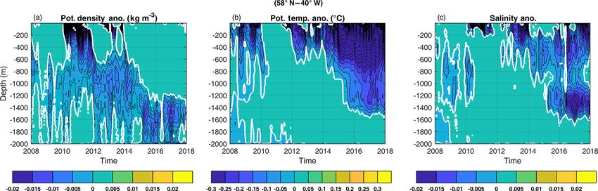
100                                        P. Zunino et al.: Deep convection SECF persisted over four consecutive winters

the small scales associated with the convection process itself,   Only data flagged as good (quality control < 3; Argo Data
Argo data allow for the description of the overall intensity      Management Team, 2017) were considered in our analysis.
of the event and the characterization of the properties of the    Potential temperature (θ ), density (ρ) and potential density
water masses formed in the winter mixed layer as well (e.g.,      anomaly referenced to the surface and 1000 dbar (σ0 and
Yashayaev and Loder, 2017).                                       σ1 , respectively) were estimated from T , S and P data us-
   In the Labrador Sea, deep convection occurs every year,        ing TEOS-10 (http://www.teos-10.org/, last access: 9 Jan-
yet with different intensity (e.g., Yashayaev and Clarke,         uary 2020).
2008; Kieke and Yashayaev, 2015). In the Irminger Sea, Argo          We used two different gridded products of ocean T and S:
and mooring data showed that convection deeper than 700 m         ISAS and EN4. ISAS (Gaillard et al., 2016; Kolodziejczyk
happened during the winters of 2008, 2009, 2012, 2015 and         et al., 2017) is produced by optimal interpolation of in situ
2016 (Väge et al., 2009; de Jong et al., 2012, 2018; Piron        data. It provides monthly fields at 152 depth levels and at
et al., 2016, 2017; de Jong and de Steur, 2016; Fröb et al.,      0.5◦ resolution from 2002 to 2015. Near-real-time data are
2016). Moreover, in winter 2015, deep convection was also         also available for 2016 and 2018. EN4 (Good et al., 2013) is
observed south of Cape Farewell (Piron et al., 2017). Exclud-     an optimal interpolation of in situ data; it provides monthly
ing winter 2009 when the deep convection event was made           T and S at 1◦ spatial resolution and at 42 depth levels for the
possible thanks to a favorable preconditioning (de Jong et        period 1900 to present.
al., 2012), all events coincided with strong atmospheric forc-       Net air–sea heat flux (Q, the sum of radiative and turbu-
ing (air–sea heat loss). Prior to 2008, only few deep convec-     lent fluxes), evaporation (E), precipitation (P ), wind stress
tion events were reported because the mechanisms leading to       (τx and τy ) and sea surface temperature (SST) data were ob-
them were not favorable (Centurioni and Gould, 2004) or be-       tained from the ERA-Interim reanalysis (Dee et al., 2011).
cause the observing system was not adequate (Bacon, 1997;         ERA-Interim provides data with a time resolution of 12 h
Pickart et al., 2003). Nevertheless, the hydrographic prop-       and a spatial resolution of 0.75◦ . The air–sea freshwater flux
erties from the 1990s suggest that deep convection reached        (FWF) was estimated as E–P .
as deep as 1500 m in the Irminger Sea during the winters of          We used monthly absolute dynamic topography (ADT),
1994 and 1995 (Pickart et al., 2003) and as deep as 1000 m        which was computed from the daily 0.25◦ resolution ADT
south of Cape Farewell during winter 1997 (Bacon et al.,          data provided by CMEMS (Copernicus Marine and Environ-
2003).                                                            ment Monitoring Service, http://www.marine.copernicus.eu,
   The convection depths that were reached in the Irminger        last access: 9 January 2020).
Sea and south of Cape Farewell at the end of winter 2015
were the deepest observed in these regions since the begin-
ning of the 21st century (de Jong et al., 2016; Piron et al.,     3     Methods
2017, Fröb et al., 2016). In this work, we show that deep
convection also happened in a region between south of Cape        3.1    Quantification of deep convection
Farewell and the Irminger Sea (the pink box in Fig. 1) every
winter from 2016 to 2018. Hereinafter, we will refer to this      We characterized the convection in the SPNA in the winters
region as southeast Cape Farewell (SECF). We investigated         of 2015–2018 by estimating the mixed layer depths (MLDs)
the respective role of atmospheric forcing (air–sea buoyancy      for all Argo profiles collected in the SPNA north of 55◦ N
flux) and preconditioning (ocean interior buoyancy content)       from 1 January to 30 April of each year (Fig. 1). The MLD
in setting the convection intensity. We also disentangled the     was estimated as the shallowest of the three MLD estimates
relative contribution of salinity and temperature anomalies to    obtained by applying the threshold method of de Boyer Mon-
the preconditioning. The paper is organized as follows. The       tégut et al. (2004) to θ , S and ρ profiles separately. The
data are described in Sect. 2. The methodology is explained       threshold method computes the MLD as the depth at which
in Sect. 3. We present our results in Sect. 4 and discuss them    the difference between the surface (30 m) and deeper lev-
in Sect. 5. Conclusions are listed in Sect. 6.                    els in a given property is equal to a given threshold. In the
                                                                  case that visual inspection of the winter profiles showed a
                                                                  thin stratified layer at the surface, a slightly deeper level
2   Data                                                          (< 150 m) was considered the surface reference level. Fol-
                                                                  lowing Piron et al. (2017), this threshold was taken as equal
We used temperature (T ), salinity (S) and pressure (P )          to 0.01 kg m−3 for ρ. For θ and S, we selected thresholds
data measured by Argo floats north of 55◦ N in the At-            of 0.1◦ C and 0.012, respectively, because they correspond
lantic Ocean. These data were collected by the International      to the threshold of 0.01 kg m−3 in ρ. The latter was previ-
Argo Program (http://www.argo.ucsd.edu/, last access: 9 Jan-      ously shown to perform well in the subpolar gyre on den-
uary 2020; http://www.jcommops.org/, last access: 9 Jan-          sity profiles (Piron et al., 2016). The criteria for tempera-
uary 2020) and downloaded from the Coriolis Data Cen-             ture and salinity were chosen to perform well when tempera-
ter (http://www.coriolis.eu.org/, last access: 9 January 2020).   ture and salinity anomalies within the density-defined mixed

Ocean Sci., 16, 99–113, 2020                                                                   www.ocean-sci.net/16/99/2020/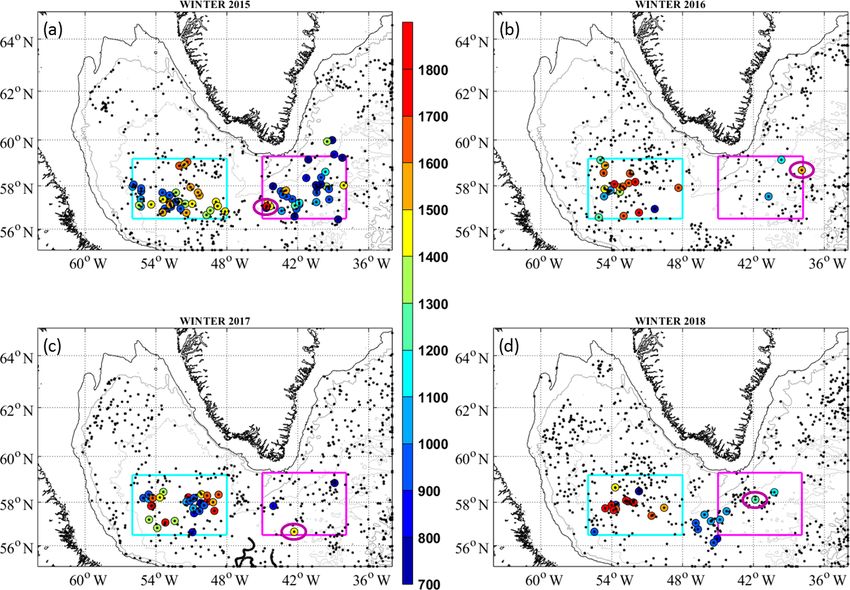
P. Zunino et al.: Deep convection SECF persisted over four consecutive winters                                                           101

Figure 1. Positions of all Argo floats north of 55◦ N in the Atlantic between 1 January and 30 April (a) 2015, (b) 2016, (c) 2017 and (d) 2018
(black and colored points). The colored points and color bar indicate the mixed layer depth (MLD) when the MLD was deeper than 700 m.
The pink circles indicate the position of the maximal MLD observed SECF each winter. The pink and cyan boxes delimit the regions used for
estimating the time series of atmospheric forcing and the vertical profiles of buoyancy to be removed in the SECF region and the Labrador
Sea, respectively (SECF: 56.5–59.3◦ N and 45.0–38.0◦ W, Labrador Sea: 56.5–59.2◦ N and 56–48◦ W).

layer are density-compensated. Our MLD estimates are com-                for each winter as the vertical mean from 200 m to the MLD
parable to those obtained using MLD determination based on               of all profiles with an MLD deeper than 700 m. For further
the Pickart et al. (2002) methods (see Sect. S1 and Figs. S1             use, we define the deep convection period as follows. For a
and S2 in the Supplement).                                               given winter, the deep convection period begins the day when
   In this paper, deep convection is characterized by profiles           the first profile with a deep (> 700 m) mixed layer is detected
with an MLD deeper than 700 m (colored points in Fig. 1) be-             and ends the day of the last detection of a deep mixed layer.
cause it is the minimum depth that should be reached for re-
newing Labrador Sea Water (LSW) (Yashayaev et al., 2007;                 3.2    Time series of atmospheric forcing
Piron et al., 2016). The winter MLD and the associated θ , S
and ρ properties were examined for the Labrador Sea and the              The air–sea buoyancy flux (Bsurf ) was calculated as the sum
SECF region by considering the profiles inside the cyan and              of the contributions of Q and FWF (Gill, 1982; Billheimer
pink boxes in Fig. 1, respectively. Those two boxes were de-             and Talley, 2013):
fined to include all Argo profiles with an MLD deeper than
                                                                                    αg
700 m during 2016–2018 and the minimum of the monthly                    Bsurf =          Q − β g SSS FWF,                                (1)
ADT for either the SECF region or the Labrador Sea. No                             ρ0 c p
deep MLD was recorded in the northernmost part of the
                                                                         where α and β are the coefficients of thermal and saline ex-
Irminger Sea during this period. We computed the maximum
                                                                         pansions, respectively, estimated from surface T and S. The
MLD and the MLD third quartile (Q3 ) from profiles with an
                                                                         gravitational acceleration g is equal to 9.8 m s−2 , the refer-
MLD greater than 700 m in each of the two boxes separately.
                                                                         ence density of sea water ρ0 is equal to 1026 kg m−3 and the
Q3 is the MLD value that is exceeded by 25 % of the profiles
                                                                         heat capacity of sea water Cp is equal to 3990 J kg −1 ◦ C−1 .
and is equivalent to the aggregate maximum depth of convec-
                                                                         SSS is the sea surface salinity (Q: W m−2 , FWF: m s−1 ).
tion defined by Yashayaev and Loder (2016). Hereafter, we
                                                                            For easy comparison with previous results, which only
refer to Q3 as the aggregate maximum depth of convection.
                                                                         considered the heat component of the buoyancy air–sea flux
The properties (ρ, θ and S) of the mixed layers were defined
                                                                         (e.g., Yashayaev and Loder, 2017; Piron et al., 2017; Rhein et

www.ocean-sci.net/16/99/2020/                                                                               Ocean Sci., 16, 99–113, 2020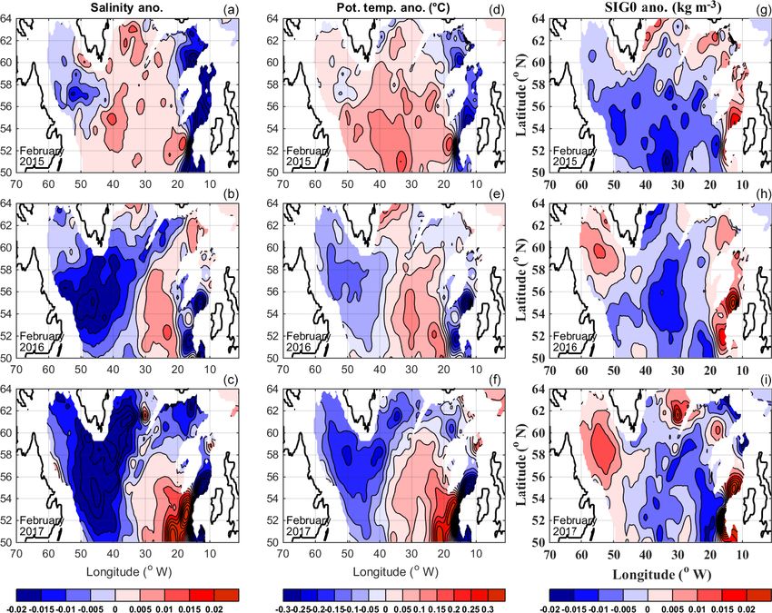
102                                       P. Zunino et al.: Deep convection SECF persisted over four consecutive winters

al., 2017), Bsurf (m2 s−3 ) was converted (W m−2 ) following    3.3    Preconditioning of the water column
                     ∗ :
Eq. (2) and noted Bsurf
                                                                The preconditioning of the water column was evaluated as
 ∗        ρ0 cp                                                 the buoyancy that has to be removed (B(zi)) from the late
Bsurf   =       Bsurf .                                   (2)
           gα                                                   summer density profile to homogenize it down to a depth zi:
                                                                                          g o
                                                                                            Z
The FWF was also converted (W m−2 ) using                                g
                                                                B (zi) =    σ0 (zi) zi −       σ0 (z)dz,                (7)
                                                                         ρ0              ρ0 zi
                          ρ0 c p
FWF∗ = FWFβSSS                   .                        (3)   where σ0 (z) is the vertical profile of potential density
                            α
                                                                anomaly estimated from the profiles of T and S measured by
We also computed the horizontal Ekman buoyancy flux             Argo floats in September in the given region (pink or cyan
(BFek ), which can be decomposed into the horizontal Ekman      box in Fig. 1).
heat flux (HFek ) and salt flux (SFek ).                          Following Schmidt and Send (2007), we split B into a tem-
                                                                perature (Bθ ) and salinity (BS ) term:
                                   Cp
BFek = −g (Ue ∂x SSD + Ve ∂y SSD)                         (4)                                     Z o
                                  α.g                           Bθ (zi) = −( g α θ (zi) zi − g α θ (z)dz),               (8)
HFek = −(Ue ∂x SST + Ve ∂y SST) ρ0 Cp                     (5)                                 Z o
                                                                                                    zi
                                β ρ0 Cp                         BS (zi) = g β S (zi) zi − g β S(z)dz.                    (9)
SFek = −(Ue ∂x SSS + Ve ∂y SSS)                           (6)
                                   α                                                           zi

BFek = SFek – HFek . Ue and Ve are the eastward and north-      In order to compare the preconditioning with the heat to be
ward components of the Ekman horizontal transport esti-         removed and/or air–sea heat fluxes, B, Bθ and BS are re-
mated from the wind stress meridional and zonal compo-          ported in Joules per square meter. B, Bθ and BS were esti-
nents. SSD, SST and SSS are ρ, T and S at the surface of        mated for a given year from the mean of all September pro-
the ocean (BFek , HFek and SFe : J s−1 m−2 ). Because ERA-      files of B, √
                                                                            Bθ and BS . The associated errors were estimated
Interim does not supply SSD or SSS, they were estimated         as std(B)/ n, where n is the number of profiles used to com-
from EN4 as follows. The monthly T and S data at 5 m of         pute the September mean values.
depth from EN4 were interpolated on the same time and
space grid as the air–sea fluxes from ERA-Interim (12 h and     4     Results
0.75◦ , respectively). SSD was estimated from those interpo-
lated EN4 data (SST and SSS). Properties at 5 m of depth        4.1    Intensity of deep convection and properties of
were considered to be representative of the Ekman layer.               newly formed LSW
Data at locations where the ocean bottom was shallower than
1000 m were excluded from the analysis to avoid regions         We examine the time evolution of the winter mixed layer
covered by sea ice.                                             SECF since the exceptional convection event of winter 2015
   Following Piron et al. (2016), the time series of atmo-      (W2015 hereinafter) (Table 1 and Figs. 1–3). In W2015,
spheric forcing were estimated for the SECF region and the      we recorded a maximum MLD of 1710 m south of Cape
Labrador Sea as follows. First, the gridded air–sea flux data   Farewell (Fig. 1a), in line with Piron et al. (2017). The max-
and the horizontal Ekman fluxes were averaged over the pink     imum MLD of 1575 m observed for W2016 (Fig. 1b) is
(SECF region) and cyan (Labrador Sea) boxes (Fig. 1). Sec-      compatible with the active mixed layer > 1500 m observed
ond, we estimated the accumulated fluxes from 1 Septem-         in a mooring array in the central Irminger Sea by de Jong
ber to 31 August the year after. Finally, we computed the       et al. (2018). For W2015 and W2016, the aggregate maxi-
time series of the anomalies of the accumulated fluxes from     mum depth of convection was 1205 and 1471 m, respectively
1 September to 31 August with respect to the 1993–2016          (Table 1). In W2017, deep convection was observed from
mean.                                                           three Argo profiles (Figs. 1c and 2a–c). The maximum MLD
   Finally, in order to quantify the net intensity of the at-   of 1400 m was observed on 16 March 2017 at 56.65◦ N–
mospheric forcing over the winter, we computed estimates        42.30◦ W. In W2018, the maximum MLD of 1300 m was
      ∗ + BF
of Bsurf                                                        observed on 24 February at 58.12◦ N, 41.84◦ W (Figs. 1d,
               ek fluxes accumulated from 1 September to
31 March the year after. Following Piron et al. (2017), the     2d–f). Float 5903102 measured an MLD of 1100 m south of
associated errors were calculated by a Monte Carlo simula-      Cape Farewell (Fig. 1d), but the estimated MLDs coincided
tion using 50 random perturbations of Q, FWF and Bsurf .        with the deepest levels of measurement of the float so that
                                                       ∗ ,Q
The error amounted to 0.05, 0.04 and 0.03 J m−2 for Bsurf       these estimates, possibly biased low (see Fig. 2d–f), were dis-
           ∗
and FWF , respectively. The error of the horizontal Ekman       carded from our analysis. These results show that convection
buoyancy transport was also estimated by a Monte Carlo sim-     deeper than 1300 m occurred during four consecutive winters
ulation and amounted to 0.04 J m−2 .                            SECF.

Ocean Sci., 16, 99–113, 2020                                                                 www.ocean-sci.net/16/99/2020/
P. Zunino et al.: Deep convection SECF persisted over four consecutive winters 103
Table 1. Properties of the deep convection SECF and in the Labrador Sea in winters 2015–2018. We show: the maximal MLD observed,
the aggregate maximum depth of convection, the σ0 , S and θ of the winter mixed layer formed during the convection event and n, which is
the number of Argo profiles indicating deep convection. The uncertainties given with σ0 , S and θ are the standard deviation of the n values
considered to estimate the mean values.
SECF Maximal MLD (m) Aggregate max. depth σ0 Salinity θ n
of convection (m)
W2015 1710 1205 27.733 ± 0.007 34.866 ± 0.013 3.478 ± 0.130 29
W2016 1575 1471 27.746 ± 0.002 34.871 ± 0.003 3.388 ± 0.032 3
W2017 1400 1251 27.745 ± 0.007 34.868 ± 0.007 3.364 ± 0.109 3
W2018 1300 1300 27.748 ± 0.001 34.859 ± 0.003 3.263 ± 0.031 2
Labrador Sea Maximal MLD Aggregate max. depth σ0 Salinity θ n
of convection (m)
W2015 1675 1504 27.733 ± 0.009 34.842 ± 0.010 3.279 ± 0.036 41
W2016 1801 1620 27.743 ± 0.006 34.836 ± 0.010 3.124 ± 0.047 18
W2017 1780 1674 27.752 ± 0.008 34.853 ± 0.009 3.172 ± 0.029 26
W2018 2020 1866 27.756 ± 0.006 34.855 ± 0.010 3.145 ± 0.083 13
Figure 2. Vertical distribution of σ0 , S and θ of Argo profiles showing an MLD deeper than 700 m SECF in winter 2017 (a, b, c) and in
winter 2018 (d, e, f). The black points indicate the MLD. The triangles in (d) are the MLD that coincided with the maximal profiling pressure
reached by the float. In the legend, the float and cycle of each profile are indicated.
Although the number of floats showing deep convection was computed for the deep convection periods defined from
in W2017 and W2018 was small (three and two floats, re- 15 January to 21 April 2015, 22 February to 21 March 2016,
spectively), it represented a significant percentage of the 16 March to 4 April 2017 and 24 February to 26 March 2018.
floats operating in the SECF box at that time. The percent- The longest period of deep convection occurred in W2015
age of floats showing deep convection in the SECF region and the shortest in 2017. The percentages of floats showing
www.ocean-sci.net/16/99/2020/ Ocean Sci., 16, 99–113, 2020104 P. Zunino et al.: Deep convection SECF persisted over four consecutive winters
deep convection during the deep convection period are 73 %, ∗ (Fig. 4a) and BF (Fig. 4d).
negative anomalies in both Bsurf ek
50 %, 33 % and 50 % for the winters of 2015, 2016, 2017 This correlation was not observed for all the years presenting
and 2018, respectively. The lowest percentage is found for a negative anomaly of atmospheric forcing. It is noteworthy
W2017, but it is still substantial. It might reflect the fact that that during W2016, W2017 and W2018, the anomaly of at-
for this specific year floats showing a deep MLD were found mospheric forcing was close to zero.
in the southwestern corner of the SECF box only, suggesting Contrary to the very negative anomaly in atmospheric
that convection did not occur over the full box. fluxes over the SECF region observed for W2015, the atmo-
The properties (σ0 , S and θ ) of the end-of-winter mixed spheric fluxes were close to the mean during W2016, W2017
layer were estimated for the four winters (Table 1 and Fig. 3). and W2018.
We observed that, between W2015 and W2018, the water
mass formed by deep convection significantly densified and 4.3 Analysis of the preconditioning of the water
cooled by 0.019 kg m−3 and 0.215 ◦ C, respectively (see Ta- column southeast of Cape Farewell
ble 1 and Fig. 3).
In the Labrador Sea, the aggregate maximum depth of con- Our hypothesis is that the exceptional deep convection that
vection increased from 2015 to 2018 (see Table 1). Deep happened in W2015 in the SECF region favorably precon-
convection observed in the Labrador Sea in W2018 was the ditioned the water column for deep convection the follow-
most intense since the beginning of the Argo era (see Fig. 2c ing winters. The time evolutions of θ , S, σ1 and 1σ1 =
in Yashayaev and Loder, 2016). From W2015 to W2018, 0.01 kg m−3 layer thicknesses (Fig. 5) show a marked change
newly formed LSW cooled, became saltier, and densified by in the hydrographic properties of the SECF region at the
0.134 ◦ C, 0.013 and 0.023 kg m−3 , respectively (Table 1). beginning of 2015 caused by the exceptional deep convec-
The water mass formed SECF is warmer and saltier than tion that occurred during W2015 (see Piron et al., 2017).
that formed in the Labrador Sea (Fig. 3). The deep convec- The intermediate waters (500–1000 m) became colder than
tion SECF is always shallower than in the Labrador Sea. This the years before, and despite a slight decrease in salinity,
result is discussed later in Sect. 5. the cooling caused the density to increase (Fig. 5c). Fig-
ure 5d shows 1σ1 = 0.01 kg m−3 layer thicknesses larger
4.2 Analysis of the atmospheric forcing southeast of than 600 m appearing at the end of W2015 for the first
Cape Farewell time since 2002. In the density range 32.36–32.39 kg m−3 ,
these layers remained thicker than ∼ 450 m during W2016
∗ and Q are in phase and of the
The seasonal cycles of Bsurf to W2018. This indicates low stratification at intermediate
same order of magnitude, while FWF∗ , which is positive depths and a favorable preconditioning of intermediate wa-
and 1 order of magnitude lower than Q, does not present a ters for deep convection initiated by W2015 deep convection.
seasonal cycle (Fig. S3). The means (1993–2018) of the cu- The denser density of the core of the thick layers in 2017–
mulative sums from 1 September to 31 March of Q, FWF∗ 2018 compared with 2015–2016 agrees with the densifica-
∗ estimated over the SECF box (Fig. 1) are −2.46 ±
and Bsurf tion of the mixed layer SECF shown in Table 1 and Fig. 3.
0.43 × 10⁹ , 0.28 ± 0.10 × 10⁹ and −2.22 ± 0.49 × 10⁹ J m−2 , B(zi) is our estimate of the preconditioning of the water
∗ is 10 % lower on average than Q because
respectively. Bsurf column before winter (see the Methods section). Figure 6a
of the buoyancy addition by FWF∗ . Considering the Ekman shows that, deeper than 100 m, B for W2016, W2017 and
transports, the 1993–2018 means of the accumulated BFek , W2018 was smaller than B for W2015 or B for the mean
HFek and SFek from 1 September to 31 March amount to W2008–W2014. Furthermore, for W2016, W2017 and 2018,
0.37±1.15×10⁸ , −0.35±1.36×10⁸ and 0.02±2.04×10⁸ × B remained nearly constant with depth between 600 and
109 J m−2 , respectively. The horizontal Ekman heat flux is 1300 m, which means that once the water column has been
negative, while the Ekman buoyancy flux is positive. This homogenized down to 600 m, little additional buoyancy loss
buoyancy gain indicates a southeastward transport of surface results in the homogenization of the water column down to
freshwater caused by dominant winds from the southwest. It 1300 m. Both conditions, (i) less buoyancy to be removed
is noteworthy that BFek is 1 order of magnitude smaller than and (ii) the absence of a gradient in the B profile down to
∗ .
the Bsurf 1300 m, indicate a more favorable preconditioning of the
The total atmospheric forcing SECF was quantified as the water column for W2016, W2017 and W2018 than during
∗ and BF . The anomalies of accumulated fluxes
sum of Bsurf W2008–W2015.
ek
from 1 September to 31 August the year after, with respect To understand the relative contributions of θ and S to the
to the mean 1993–2016, are displayed in Fig. 4 for the SECF preconditioning, we computed the thermal (Bθ ) and haline
box. The gray line in Fig. 4a is the total atmospheric forc- (BS ) components of B (B = Bθ + BS ). In general, Bθ (BS )
∗ plus BF ). We identify years with very
ing anomaly (Bsurf increases with depth when θ decreases (S increases) with
ek
negative buoyancy loss in the SECF region, e.g., 1994, 1999, depth. On the contrary, a negative slope in a Bθ (BS ) profile
2008, 2012 and 2015. The very negative anomalies of atmo- corresponds to θ increasing (S decreasing) with depth and
spheric forcing in 1999 and 2015 were caused by the very is indicative of a destabilizing effect. The negative slopes in
Ocean Sci., 16, 99–113, 2020 www.ocean-sci.net/16/99/2020/P. Zunino et al.: Deep convection SECF persisted over four consecutive winters 105
Figure 3. TS diagrams in the mixed layer for profiles with an MLD deeper than 700 m during the winters of 2015, 2016, 2017 and 2018 for
(a) the Labrador Sea and (b) SECF. The properties of the mixed layers were estimated as the vertical means between 200 m and the MLD.
Bθ and BS profiles are not observed simultaneously because in Fig. 7a) than for the mean 2008–2014 (1000 m; see blue
density profiles are stable. dashed line in Fig. 7a). Finally, we note that the profiles of
We describe the relative contributions of Bθ and BS to B B(zi ), Bθ (zi ) and BS (zi ) for W2016 and W2018 are more
by looking first at the mean 2008–2014 profiles (discontin- similar to the profiles of W2017 than to those of W2015
uous blue lines in Fig. 6). Bθ accounts for most of the in- or to the mean 2008–2014 (see Fig. 6), which indicates that
crease in B from the surface to 800 m and below 1400 m (see the water column was also favorably preconditioned for deep
Fig. 6a and b). The negative slope in the BS profile between convection in W2016 and W2018 for the same reasons as in
800 and 1000 m (Fig. 6c) slightly reduces B (Fig. 6a) and W2017.
is due to the decrease in S associated with the core of LSW The origin of the changes in B is now discussed from the
(see Fig. 3 in Piron et al., 2016). In the layer 1000–1400 m, time evolutions of the monthly anomalies of θ , S and σ0 at
the increase in B (Fig. 6a) is mainly explained by the in- 58◦ N–40◦ W, which is at the center of the SECF box (Fig. 8).
crease in BS (Fig. 6c), which follows the increase in S in The time evolutions there are similar to those at any other
the transition from LSW to Iceland Scotland Overflow Water location inside the SECF box. These anomalies were com-
(ISOW). This transition layer will be referred to hereinafter puted using ISAS Gaillard et al., 2016) and were referenced
as the deep halocline. The preconditioning of the water col- to the monthly mean of 2002–2016. A positive anomaly
umn is usually analyzed in terms of heat (e.g., Piron et al., of σ0 appeared in 2014 between the surface and 600 m
2015, 2017). The decomposition of B in Bθ and BS reveals (Fig. 8a) and reached 1200 m in 2015 and beyond. This pos-
that θ governs B in the layer 0–800 m. S tends to reduce the itive anomaly of σ0 correlates with a negative anomaly of
stabilizing effect of θ in the layer 800–1000 m and reinforces θ . The latter, however, reached ∼ 1400 m of depth in 2016,
it in the layer 1000–1400 m by adding up to 1 × 10⁹ J m2 to which is deeper than the positive anomaly of σ0 . The nega-
B. tive anomaly of S between 1000 and 1500 m that appeared
In order to further understand why the SECF region was in 2015 and strongly reinforced in 2016 caused the nega-
favorably preconditioned during the winters of 2016–2018, tive anomaly in σ0 between 1200 and 1500 m (the density
we compare the Bθ and BS of W2017, which was the most anomaly caused by the negative anomaly in θ between 1200
favorably preconditioned winter, with the mean 2008–2014 and 1400 m does not balance the density anomaly caused by
(Fig. 7a). From the surface to 1600 m, Bθ and BS were the negative anomaly of S).
smaller for W2017 than for the mean 2008–2014. There are The θ and S anomalies in the water column during 2016–
two additional remarkable features. First, in the layer 500– 2018 explain the anomalies of B, Bθ and BS and can be
1000 m, the large reduction of Bθ compared to the 2008– summarized as follows. On the one hand, the properties of
2014 mean mostly explains the decrease in B in this layer. the surface waters (down to 500 m) were colder than previ-
Second, the more negative value of BS in the layer 1100– ous years and, despite the fact that they were also fresher,
1300 m, compared to the 2008–2014 mean, eroded the Bθ they were denser. The density increase in the surface water
slope, making the B profile more vertical for W2017 than reduced the density difference with the deeper-lying waters.
for the mean. The more negative contribution of BS in the The intermediate layer (500–1000 m) was also favorably pre-
layer 1100–1300 m comes from the fact that the deep halo- conditioned due to the observed cooling. Additionally, in the
cline was deeper for W2017 (1300 m; see orange dashed line layer 1100–1300 m, the large negative anomaly of BS with
www.ocean-sci.net/16/99/2020/ Ocean Sci., 16, 99–113, 2020106 P. Zunino et al.: Deep convection SECF persisted over four consecutive winters
Figure 4. Time series of anomalies of accumulated (a) Bsurf∗ , (b) Q, (c) FWF∗ (d) BF , (e) HF and (f) SF averaged in the SECF
ek ek ek
region. They are anomalies with respect to 1993–2016. The accumulation was from 1 September to 31 August the following year. The winter
North Atlantic Oscillation (NAO) index (Hurrell et al., 2018) is also represented in (g). The gray line in (a) is the sum of the anomalies of
∗ and BF . Note that the range of values in the y axis is not the same in all the plots.
accumulated Bsurf ek
Ocean Sci., 16, 99–113, 2020 www.ocean-sci.net/16/99/2020/P. Zunino et al.: Deep convection SECF persisted over four consecutive winters 107
Figure 5. Time evolutions of vertical profiles measured from Argo floats in the SECF region: (a) θ, (b) S, (c) σ1 and (d) the thickness
of 0.01 kg m−3 thick σ1 layers. The white horizontal bars in plots (a), (b) and (c) indicate the maximal convection depth observed in the
Irminger Sea or SECF when deep convection occurred. The white line in plot (a) indicates the depth of the isotherm 3.6 ◦ C. The black vertical
ticks on the x axes of plot (b) indicate times of Argo measurements. These figures were created from all Argo profiles reaching deeper than
1000 m in the SECF region (56.5–59.3◦ N, 45–38◦ W; pink box in Fig. 1). The yearly numbers of Argo profiles used in this figure are shown
in Fig. S5.
respect to its mean is explained by the decrease in S in this served MLD within ±200 m. The differences could be due to
layer, which caused a decrease in σ0 and consequently re- errors in the atmospheric forcing (Josey et al., 2018), lateral
duced the σ0 difference with the shallower-lying water. The advection and/or spatial variation in the convection intensity
decrease in S also resulted in a deepening of the deep halo- within the box not captured by the Argo sampling.
cline. The satisfactory predictability of the convection depth
with our 1-D model indicates that deep convection oc-
4.4 Atmospheric forcing versus preconditioning of the curred locally. In spite of the fact that the atmospheric
water column forcing was close to mean (1993–2016) conditions during
W2016, W2017 and W2018, convection depths > 1300 m
We now use the estimates of the accumulated atmospheric were reached in the SECF region. This was only possible
∗ +BF ) from 1 September to 31 March the year
forcing (Bsurf thanks to the favorable preconditioning.
ek
after (see Fig. S4) to predict the maximum convection depth
for a given winter based on September profiles of B. The pre-
dicted convection depth is determined as the depth at which 5 Discussion
B(zi) (Fig. 6a) equals the accumulated atmospheric forcing.
The associated error was estimated by propagating the error Deep convection happens in the Irminger Sea and south of
in the atmospheric forcing (0.05 × 10⁹ J m−2 ). The accumu- Cape Farewell during specific winters characterized by a
lated atmospheric forcing amounted to −3.21 × 10⁹ ± 0.05 strong atmospheric forcing (high buoyancy loss), a favorable
−2.21 ± 0.04 × 10⁹ , −2.01 ± 0.05 × 10⁹ and −2.47 ± 0.05 × preconditioning (low stratification) or both at the same time
109 J m−2 for W2015, W2016, W2017 and W2018, respec- (Bacon et al., 2003; Pickart et al., 2003). In the Irminger Sea,
tively. We found predicted convection depths of 1085 ± 20, strong atmospheric forcing explained, for instance, the very
1285 ± 20, 1415 ± 20 and 345 ± 20 m for W2015, W2016, deep convection (reaching depths greater than 1500 m) ob-
W2017 and W2018, respectively. We consider the aggregate served in the early 1990s (Pickart et al., 2003) and in W2015
maximum depth of convection to be the observed estimate of (de Jong et al. 2016; Fröb et al., 2016; Piron et al., 2017). It
the MLD (Table 1). The predicted MLD agrees with the ob- also explained the return of deep convection in W2008 (Väge
www.ocean-sci.net/16/99/2020/ Ocean Sci., 16, 99–113, 2020108 P. Zunino et al.: Deep convection SECF persisted over four consecutive winters Figure 6. Vertical profile of (a) the buoyancy to be removed (B), (b) the thermal component (Bθ ) and (c) the salinity component (BS ). They were calculated from all Argo data measured in the SECF box (see Fig. 1) in September before the winter indicated in the legend. For W2015 and W2018, we considered data from 15 August to 30 September 2017 because not enough data were available in September. The number of Argo profiles taken into account to estimate the B profiles was more than 10 for all the winters. et al., 2009) and in W2012 (Piron et al., 2016). The favor- originated locally during W2015 when extraordinary deep able preconditioning caused by the densification of the mixed convection happened. A slight freshening of the water col- layer during W2008 favored a new deep convection event in umn (400–1500 m) appeared in 2015, likely caused by the W2009 despite neutral atmospheric forcing (de Jong et al., W2015 convection event; then it decreased before a second 2012). Similarly, the preconditioning observed after W2015 S anomaly intensified in 2016 between 1100 and 1400 m in the SECF region favored deep convection in W2016 (this (Fig. 8c). It is unlikely that this second anomaly was ex- work). The favorable preconditioning persisted for three con- clusively locally formed by deep convection because it in- secutive winters (2016–2018) in the SECF region, which tensified during summer 2016. Our hypothesis is that this allowed deep convection although atmospheric forcing was second S anomaly originated in the Labrador Sea and was close to the climatological values. Why did this favorable further transferred to the SECF region by the cyclonic circu- preconditioning persist in time? lation encompassing the Labrador Sea and Irminger Sea at We previously showed that during 2016–2018 two hydro- these depths (Daniault et al., 2016; Ollitrault and Colin de graphic anomalies affected different ranges of the water col- Verdière, 2014; Lavander et al., 2000; Straneo et al., 2003). umn in the SECF box: a cooling intensified in the layer 200– This is corroborated by the 2-D evolution of the anomalies in 800 m and a freshening intensified in the 1000–1500 m layer. S in the layer 1200–1400 m (Fig. 9): a negative anomaly in S Those resulted in a decrease in the vertical density gradient appeared in the Labrador Sea in February 2015, which was between the intermediate and the deeper layers, creating a transferred southward and northeastward in February 2016 favorable preconditioning of the water column. Note that the and intensified over the whole SPNA in February 2017. By cooling affected the layer from the surface to 1400 m, and the this mechanism, the advection from the Labrador Sea con- freshening affected the layer from the near surface to 1600 m, tributed to create property anomalies in the water column. but the cooling and the freshening were intensified at differ- However, the buoyancy budget showed that this was a minor ent depth ranges (Fig. 8). contribution compared to the buoyancy loss due to the local We see in Fig. 5a a sudden decrease in θ in the interme- air–sea flux, even if it was essential to preconditioning the diate layers in 2015 compared to the previous years. It indi- water column for deep convection. cates that the decrease in θ of the intermediate layer likely Ocean Sci., 16, 99–113, 2020 www.ocean-sci.net/16/99/2020/
P. Zunino et al.: Deep convection SECF persisted over four consecutive winters 109
Figure 7. Decomposition of the profiles of buoyancy to be removed (B, continuous lines) in its thermal (Bθ , dotted lines) and salinity (BS ,
dashed lines) components in (a) the SECF region; (b) the Labrador Sea. The BS components for W2016 and W2018 were added to show the
evolution of the depth of the deep halocline.
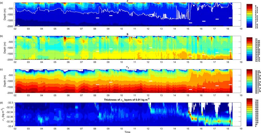
Figure 8. Evolution of vertical profiles of monthly anomalies of (a) σ0 , (b) θ and (c) S at 58◦ N, 40◦ W. The anomalies were estimated from
the ISAS database (Gaillard et al., 2016) and were referenced to the monthly mean estimated for 2002–2016.
We now compare the atmospheric forcing and the pre- the Labrador Sea and −2.18 ± 0.54 × 10⁹ J m−2 in the SECF
conditioning of the water column in the SECF region with region. The difference was larger during the period 2016 –
those of the nearby Labrador Sea where deep convection hap- 2018 when the atmospheric forcing equaled −3.10 ± 0.19 ×
pens almost every year. The atmospheric forcing over the 109 J m−2 in the Labrador Sea and −2.23 ± 0.23 × 10⁹ J m−2
Labrador Sea is ∼ 15 % larger than that over the SECF re- in the SECF region. In terms of preconditioning, the 2008–
gion: the means (1993–2018) of the atmospheric forcing, de- 2014 mean B profile (blue continuous lines in Fig. 7) was
∗ +BF from 1 September
fined as the time-accumulated Bsurf ek lower by ∼ 0.5 × 10⁹ J m−2 in the Labrador Sea than SECF
to 31 March the year after, are −2.61 ± 0.55 × 10⁹ J m−2 in for the surface to the 1000 m layer and by more than 1 ×
www.ocean-sci.net/16/99/2020/ Ocean Sci., 16, 99–113, 2020110 P. Zunino et al.: Deep convection SECF persisted over four consecutive winters Figure 9. Horizontal distribution of the anomalies of S (a, b, c), θ (d, e, f) and σ0 (g, h, i) in the layer 1200–1400 m in February 2015 (a, d, g), February 2016 (b, e, h) and February 2017 (c, f, i). The monthly anomalies were estimated from the ISAS database and were referenced to the period 2002–2016. 109 J m−2 below 1200 m. This indicates that the water col- those of Yashayaev and Loader, 2017). In contrast, in the umn was more favorably preconditioned in the Labrador Sea SECF region during the same period, the atmospheric forcing than in the SECF region during 2008–2014. Differently, B was close to climatological values, and the favorable precon- for W2017 shows slightly lower values from the surface to ditioning of the water column allowed for 1300 m of depth 1300 m in the SECF region than in the Labrador Sea (see convection, which was exceptional for the SECF region. orange lines in Fig. 7). However, B in the Labrador Sea The Labrador Sea, SECF region and Irminger Sea are three remains constant down to the depth of the deep halocline distinct deep convection sites (e.g., Yashayaev et al., 2007; between LSW and North Atlantic Deep Water (NADW) at Bacon et al., 2003; Pickart et al., 2003; Piron et al., 2017). In 1700 m. In the SECF region, the deep halocline remained at this work, we give new insights on the connections between ∼ 1300 m between 2016 and 2018 (see BS lines in Fig. 7a). the different sites, showing how the lateral advection of fresh Differently, in the Labrador Sea, the deep halocline deep- LSW formed in the Labrador Sea favored the precondition- ened from 1200 m for the mean to 1735, 1775 and 1905 m ing in the SECF region, fostering deeper convection. in W2016, W2017 and W2018, respectively (see the dashed Climate models forecast an increasing input of freshwater lines in Fig. 7b). The deep halocline acts as a physical bar- in the North Atlantic due to ice melting under present cli- rier for deep convection in both the SECF region and the mate change (Bamber et al., 2018), which could reduce or Labrador Sea, but because the deep halocline is deeper in even shut down the deep convection in the North Atlantic the Labrador Sea than in the SECF region, the precondition- (Yang et al., 2016; Brodeau and Koenigk, 2016). We ob- ing is more favorable to a deeper convection in the Labrador served a fresh anomaly in the surface waters in regions close Sea than in the SECF region. Summarizing, in the winters to the eastern coast of Greenland in 2016 that extended to of 2016–2018 in the Labrador Sea, both atmospheric forc- the whole Irminger Sea in 2017 (Fig. S6). However, this sur- ing and preconditioning of the water column allowed for the face freshening did not hamper the deep convection in the deepest convection depth in the Labrador Sea since the be- SECF region, possibly because the surface water also cooled. ginning of the Argo period (comparison of our results with Swingedouw et al. (2013) indicated that the freshwater signal Ocean Sci., 16, 99–113, 2020 www.ocean-sci.net/16/99/2020/
P. Zunino et al.: Deep convection SECF persisted over four consecutive winters                                                    111

due to Greenland ice sheet melting is mainly accumulating        LSW formed in the Labrador Sea. The S anomaly of this
in the Labrador Sea. However, no negative anomaly of S was       layer resulted in a deeper deep halocline. Hence, the cooling
detected in the surface waters of the Labrador Sea (Fig. S6).    of the intermediate water was essential to reach a convection
It might be explained by the intense deep convection affect-     depth of 800–1000 m, and the freshening in the layer 1200–
ing the Labrador Sea since 2014 that could have transferred      1400 m and the associated deepening of the deep halocline
the surface freshwater anomaly to the ocean interior. This       allowed for very deep convection (> 1300 m) in W2016–
suggests that, in the last years, the interactions between ex-   W2018.
pected climate change anomalies and the natural dynamics
of the system combined to favor very deep convection. This,
however, does not foretell the long-term response to climate     Data availability. The Argo data were collected and made freely
change.                                                          available by the International Argo Program and the national pro-
                                                                 grams that contribute to it (https://doi.org/10.17882/42182;
                                                                 Argo group, 2019). The ISAS data were downloaded
                                                                 from the SEANOE site (https://doi.org/10.17882/52367;
6   Conclusions
                                                                 Kolodziejczyk et al., 2017). The EN4 data are available at http:
                                                                 //hadobs.metoffice.com/en4/download.html (Good et al., 2013).
During 2015–2018 winter deep convection happened in the          The ERA-Interim data are available at https://www.ecmwf.int/en/
SECF region, reaching deeper than 1300 m. The deep con-          forecasts/datasets/reanalysis-datasets/era-interim (Dee et al., 2011).
vection of W2015 was observed over a larger region and dur-      The NAO data were downloaded from the UCAR Climate Data
ing a longer period of time than the deep convection events      Guide website (https://climatedataguide.ucar.edu/climate-data/
of the winters of 2016, 2017 and 2018. Despite these differ-     hurrell-north-atlantic-oscillation-nao-index-station-based,       last
ences, it is the first time that deep convection, with a maxi-   access: 9 January 2020; Hurrell et al., 2018). The Ssalto/Duacs
mum convection depth greater than 1300 m, was observed in        altimeter products were produced and distributed by the Coper-
this region during four consecutive winters.                     nicus Marine and Environment Monitoring Service (CMEMS)
   The atmospheric forcing and preconditioning of the water      (http://marine.copernicus.eu/services-portfolio/access-to-products/
                                                                 ?option=com_csw&view=details&product_id=SEALEVEL_
column were evaluated in terms of buoyancy. We showed that
                                                                 GLO_PHY_L4_REP_OBSERVATIONS_008_047, last access:
the atmospheric forcing is 10 % weaker when evaluated in
                                                                 9 January 2020).
terms of buoyancy than in terms of heat because of the non-
negligible effect of the freshwater flux. The analysis of the
preconditioning of the water column in terms of buoyancy to      Supplement. The supplement related to this article is available on-
be removed (B) and its thermal and salinity terms (Bθ and        line at: https://doi.org/10.5194/os-16-99-2020-supplement.
BS ) revealed that Bθ dominated the B profile from the sur-
face to 800 m, and BS reduced the B in the 800–1000 m layer
because of the low salinity of LSW. Deeper, BS increased B       Author contributions. PZ treated and analyzed the data. PZ and
due to the deep halocline (LSW–ISOW) that acted as a phys-       HM interpreted the results. PZ, HM and VT discussed the results
ical barrier limiting the depth of the convection.               and wrote the paper.
   During 2016–2018, the air–sea buoyancy losses were close
to the climatological values, and very deep convection was
possible thanks to the favorable preconditioning of the water    Competing interests. The authors declare that they have no conflict
column. It was surprising that these events reached convec-      of interest.
tion depths similar to those observed in W2012 and W2015,
when the latter were caused by high air–sea buoyancy loss
intensified by the effect of strong wind stress. It was also     Acknowledgements. We thank all the navy staff and PIs contribut-
surprising that the water column remained favorably precon-      ing to the deployment of Argo floats; without them this work would
                                                                 not be possible. We thank Marieke Femke de Jong and two anony-
ditioned during three consecutive winters without strong at-
                                                                 mous reviewers; their comments and suggestions have enriched our
mospheric forcing. In this paper, we studied the reasons why
                                                                 work.
this happened.
   The preconditioning for deep convection during 2016–
2018 was particularly favorable due to the combination           Financial support. This paper is a contribution to the EQUIPEX
of two types of hydrographic anomalies affecting differ-         NAOS project funded by the French National Research Agency
ent depth ranges. First, the surface and intermediate wa-        (ANR) under reference ANR-10-EQPX-40.
ters (down to 800 m) were favorably preconditioned because
buoyancy (density) decreased (increased) due to the cooling
caused by the atmospheric forcing. Second, buoyancy (den-        Review statement. This paper was edited by Neil Wells and re-
sity) increased (decreased) in the layer 1200–1400 m due to      viewed by Femke de Jong and two anonymous referees.
the decrease in S caused by the lateral advection of fresher

www.ocean-sci.net/16/99/2020/                                                                       Ocean Sci., 16, 99–113, 2020
112 P. Zunino et al.: Deep convection SECF persisted over four consecutive winters
References injects oxygen and anthropogenic carbon to the ocean interior,
Nat. Commun., 7, 13244, https://doi.org/10.1038/ncomms13244,
Argo Data Management Team: Argo user’s manual V3.2, 2016.
https://doi.org/10.13155/29825, 2017. Gaillard, F., Reynaud, T., Thierry, V., Kolodziejczyk, N., and
Argo group: Argo float data and metadata from Global Von Schuckmann, K.: In situ-based reanalysis of the global
Data Assembly Centre (Argo GDAC), SEANOE, ocean temperature and salinity with ISAS: Variability of the
https://doi.org/10.17882/42182, 2019. heat content and steric height, J. Climate, 29, 1305–1323,
Bacon, S.: Circulation and Fluxes in the North At- https://doi.org/10.1175/JCLI-D-15-0028.1, 2016.
lantic between Greenland and Ireland, J. Phys. Gill, A. E.: Atmosphere-Ocean Dynamics, vol. 30, Academic, San
Oceanogr., 27, 1420–1435, https://doi.org/10.1175/1520- Diego, CA, 1982.
0485(1997)0272.0.CO;2, 1997. Good, S. A., Martin, M. J., and Rayner, N. A.: EN4:
Bacon, S., Gould, W. J., and Jia, Y.: Open-ocean convec- Quality controlled ocean temperature and salinity pro-
tion in the Irminger Sea, Geophys. Res. Lett., 30, 1246, files and monthly objective analyses with uncertainty
https://doi.org/10.1029/2002GL016271, 2003. estimates, J. Geophys. Res.-Oceans, 118, 6704–6716,
Bamber, J. L., Tedstone, A. J., King, M. D., Howat, I. M., En- https://doi.org/10.1002/2013JC009067, 2013 (data avail-
derlin, E. M., van den Broeke, M. R., and Noel, B.: Land Ice able at: http://hadobs.metoffice.com/en4/download.html, last
Freshwater Budget of the Arctic and North Atlantic Oceans: access: 9 January 2020).
1. Data, Methods, and Results, J. Geophys. Res.-Oceans, 123, Hurrell, J. and National Center for Atmospheric Research
https://doi.org/10.1002/2017JC013605, 2018. Staff (Eds.): The Climate Data Guide: Hurrell North
Billheimer, S. and Talley, L. D.: Near cessation of Eighteen De- Atlantic Oscillation (NAO) Index (station-based), avail-
gree Water renewal in the western North Atlantic in the warm able at: https://climatedataguide.ucar.edu/climate-data/
winter of 2011–2012, J. Geophys. Res.-Oceans, 118, 6838–6853, hurrell-north-atlantic-oscillation-nao-index-station-based
https://doi.org/10.1002/2013JC009024, 2013. (last access: 28 June 2018), 2018.
Brodeau, L. and Koenigk, T.: Extinction of the northern oceanic Josey, S. A., Hirschi, J. J.-M., Sinha, B., Duchez, A., Grist,
deep convection in an ensemble of climate model simulations J. P., and Marsh, R.: The Recent Atlantic Cold Anomaly:
of the 20th and 21st centuries, Clim. Dynam., 46, 2863–2882, Causes, Consequences, and Related Phenomena, Annu. Rev.
https://doi.org/10.1007/s00382-015-2736-5, 2016. Mar. Sci., 10, 475–501, https://doi.org/10.1146/annurev-marine-
Centurioni and Gould, W. J.: Winter conditions in the Irminger Sea 121916-063102, 2018.
observed with profiling floats, J. Marine Res., 62, 313–336, 2004. Kieke, D. and Yashayaev, I.: Studies of Labrador Sea Water for-
Daniault, N., Mercier, H., Lherminier, P., Sarafanov, A., mation and variability in the subpolar North Atlantic in the light
Falina, A., Zunino, P., and Gladyshev, S.: The north- of international partner and collaboration, Prog. Oceanogr., 132,
ern North Atlantic Ocean mean circulation in the 220–232, https://doi.org/10.1016/j.pocean.2014.12.010, 2015.
early 21st century, Prog. Oceanogr., 146, 142–158, Kolodziejczyk, N., Prigent-Mazella, A., and Gaillard, F.:
https://doi.org/10.1016/j.pocean.2016.06.007, 2016. ISAS-15 temperature and salinity gridded fields, Seanoe,
de Boyer Montégut, C., Madec, G., Fischer, A. S., Lazar, https://doi.org/10.17882/52367, 2017.
A., and Iudicone, D.: Mixed layer depth over the global Lavender, K. L., Davis, R. E., and Owens, W. B.: Mid-depth recir-
ocean: An examination of profile data and a profile- culation observed in the interior Labrador and Irminger seas by
based climatology, J. Geophys. Res.-Oceans, 109, 1–20, direct velocity measurements, Nature, 407, 2000.
https://doi.org/10.1029/2004JC002378, 2004. Marshall, J. and Schott, F.: Open-Ocean Convection The-
de Jong, M. F. and de Steur, L.: Strong winter cooling over the ory, and Models Observations, Rev. Geophys., 37, 1–64,
Irminger Sea in winter 2014–2015, exceptional deep convection, https://doi.org/10.1029/98RG02739, 1999.
and the emergence of anomalously low SST, Geophys. Res. Lett., Ollitrault, M. and Colin de Verdière, A.: The Ocean General Cir-
43, 7106–7113, https://doi.org/10.1002/2016GL069596, 2016. culation near 1000-m Depth, J. Phys. Oceanogr., 44, 384–409,
de Jong, M. F., Van Aken, H. M., Våge, K., and Pickart, https://doi.org/10.1175/JPO-D-13-030.1, 2014.
R. S.: Convective mixing in the central Irminger Pickart, R. S., Torres, D. J., and Clarke, R. A.: Hydrography of the
Sea: 2002–2010, Deep-Sea Res. Pt. I, 63, 36–51, Labrador Sea during active convection, J. Phys. Oceanogr., 32,
https://doi.org/10.1016/j.dsr.2012.01.003, 2012. 428–457, 2002.
de Jong, M. F., Oltmanns, M., Karstensen, J., and de Steur, Pickart, R. S., Straneo, F., and Moore, G. W. K.: Is Labrador Sea
L.: Deep Convection in the Irminger Sea Observed Water formed in the Irminger basin?, Deep-Sea Res. Pt. I, 50,
with a Dense Mooring Array, Oceanography, 31, 50–59, 23–52, https://doi.org/10.1016/S0967-0637(02)00134-6, 2003.
https://doi.org/10.5670/oceanog.2018.109, 2018. Piron, A., Thierry, V., Mercier, H., and Caniaux, G.: Argo float ob-
Dee, D. P., Uppala, S. M., Simmons, A. J., Berrisford, P., Poli, P., servations of basin-scale deep convection in the Irminger sea
Kobayashi, S., and Vitart, F.: The ERA-Interim reanalysis: Con- during winter 2011–2012, Deep-Sea Res. Pt. I, 109, 76–90,
figuration and performance of the data assimilation system, Q. J. https://doi.org/10.1016/j.dsr.2015.12.012, 2016.
Roy. Meteor. Soc., 137, 553–597, https://doi.org/10.1002/qj.828, Piron, A., Thierry, V., Mercier, H., and Caniaux, G.: Gyre-scale
2011 (data available at: https://www.ecmwf.int/en/forecasts/ deep convection in the subpolar North Atlantic Ocean dur-
datasets/reanalysis-datasets/era-interim, last access: 9 Jan- ing winter 2014–2015, Geophys. Res. Lett., 44, 1439–1447,
uary 2020). https://doi.org/10.1002/2016GL071895, 2017.
Fröb, F., Olsen, A., Våge, K., Moore, G. W. K., Yashayaev, I.,
Jeansson, E., and Rajasakaren, B.: Irminger Sea deep convection
Ocean Sci., 16, 99–113, 2020 www.ocean-sci.net/16/99/2020/P. Zunino et al.: Deep convection SECF persisted over four consecutive winters 113 Rhein, M., Steinfeldt, R., Kieke, D., Stendardo, I., and Yashayaev, Yang, Q., Dixon, T. H., Myers, P. G., Bonin, J., Cham- I.: Ventilation variability of Labrador Sea Water and its impact bers, D., and Van Den Broeke, M. R.: Recent increases on oxygen and anthropogenic carbon: a review, Philos. T. Roy. in Arctic freshwater flux affects Labrador Sea convection Soc. A, 375, 20160321, https://doi.org/10.1098/rsta.2016.0321, and Atlantic overturning circulation, Nat. Commun., 7, 1–7, 2017. https://doi.org/10.1038/ncomms10525, 2016. Schmidt, S. and Send, U.: Origin and Composition of Seasonal Yashayaev, I. and Clarke, A.: Evolution of North Atlantic Water Labrador Sea Freshwater, J. Phys. Oceanogr., 37, 1445–1454, Masses Inferred From Labrador Sea Salinity Series, Oceanogra- https://doi.org/10.1175/JPO3065.1, 2007. phy, 21, 30–45, https://doi.org/10.5670/oceanog.2008.65, 2008. Straneo, F, Pickart, R. S., and Lavender, K.: Spreading of Labrador Yashayaev, I. and Loder, J. W.: Recurrent replenishment sea water: an advective-diffusive study based on Lagrangian data, of Labrador Sea Water and associtated decadal-scale Deep-Sea Res. Pt. I, 50, 701–719, 2003. variability, J. Geophys. Res.-Oceans, 121, 8095–8114, Swingedouw, D., Rodehacke, C. B., Behrens, E., Menary, M., https://doi.org/10.1002/2016JC012046, 2016. Olsen, S. M., and Gao, Y.: Decadal fingerprints of freshwater dis- Yashayaev, I. and Loder, J. W.: Further intensification of deep con- charge around Greenland in a multi-model ensemble, Clim, Dy- vection in the Labrador Sea in 2016, Geophys. Res. Lett., 44, nam., 41, 695–720, https://doi.org/10.1007/s00382-012-1479-9, 1429–1438, https://doi.org/10.1002/2016GL071668, 2017. 2013. Yashayaev, I., Bersch, M., and van Aken, H. M.: Spreading of the Våge, K., R. S. Pickart, V. Thierry, G. Reverdin, C. M. Lee, B. Labrador Sea Water to the Irminger and Iceland basins, Geophys. Petrie, T. A. Agnew, A. Wong, and M. H. Ribergaard: Sur- Res. Lett., 34, 1–8, https://doi.org/10.1029/2006GL028999, prising return of deep convection to the subpolar North At- 2007. lantic Ocean in winter 2007–2008, Nat. Geosci., 2, 67–72, https://doi.org/10.1038/ngeo382, 2009. www.ocean-sci.net/16/99/2020/ Ocean Sci., 16, 99–113, 2020
You can also read