Past and Future Spatial Growth Dynamics of Chihuahua City, Mexico: Pressures for Land Use
←
→
Page content transcription
If your browser does not render page correctly, please read the page content below
International Journal of
           Geo-Information

Article
Past and Future Spatial Growth Dynamics of
Chihuahua City, Mexico: Pressures for Land Use
Jesús A. Prieto-Amparán 1 , Alfredo Pinedo-Alvarez 2 , Federico Villarreal-Guerrero 2, *,
Carmelo Pinedo-Alvarez 2 , Carlos Morales-Nieto 2 and Carlos Manjarrez-Domínguez 3
 1    Graduate Student, Facultad de Zootecnia y Ecología, Universidad Autónoma de Chihuahua, Chihuahua,
      Chih. 31453, Mexico; jesus_prieto06@hotmail.com
 2    Facultad de Zootecnia y Ecología, Universidad Autónoma de Chihuahua, Chihuahua, Chih. 31453, Mexico;
      apinedoa@gmail.com (A.P.-A.); cpinedo@uach.mx (C.P.-A.); cnieto@uach.mx (C.M.-N.)
 3    Facultad de Ciencias Agrotecnológicas, Universidad Autónoma de Chihuahua, Chihuahua, Chih. 31310,
      Mexico; carlosmd23@hotmail.com
 *    Correspondence: fvillarreal@uach.mx; Tel.: +52-614-4-34-03-63 (ext. 15)

 Academic Editors: Qiming Zhou and Wolfgang Kainz
 Received: 18 August 2016; Accepted: 1 December 2016; Published: 8 December 2016
 Abstract: In this study, the transitions of land use that occurred in the urban and peripheral areas of
 Chihuahua City, Mexico, were determined for the period 1989–2014. Landsat TM and OLI scenes,
 as well as the method of Markov Chains (MC) were used. Grasslands and Shrublands were the
 land uses that experienced the highest pressures for land use. Grasslands occupied 23.5% of the
 area in 1989, decreasing to 16.01% in 2014. Likewise, Shrublands were reduced from 54.53% to
 48.06%. The areas occupied by Croplands, Oak forest, Water bodies and Riparian vegetation stayed
 in general constant. In contrast, the urban area increased from 13.6% to 28.6% of the total area studied.
 In addition, projections of land use for 2019 and 2024 were generated through the method of MC
 and Cellular Automata (CA). According to the projections, validated with an agreement of 0.90,
 the Human settlements would continue to expand, occupying 38.57% by 2019 and almost half of the
 studied territory (47.33%) by 2024. The ecosystems with the highest pressure for land use change will
 continue to be the Grasslands and Shrublands. By 2024, the former would lose 15.8% while the latter
 would lose 16.7% of the area. These methods are valuable for urban planning and the results could
 support growth plans for Chihuahua City, Mexico, with a sustainable approach.

 Keywords: land use change; Markov; Cellular Automata; transition matrix

1. Introduction
     The increase in population and urbanization is one of the most complex processes because it
involves changes in land use and vegetation at local, regional and global scales [1,2]. Although urban
areas cover only 2% of the planet’s surface, they have significantly altered the natural landscape [3–6].
During the last decade, urban sprawl has become a topic of particular interest due to the accelerated
growth of human settlements on the planet and the great impact involved in the phenomenon [7–10].
     Cities are responsible for the production of 78% of the greenhouse gases, contributing significantly
to global climate change [11]. Other effects of urbanization include alteration of the biogeochemical
cycles [12] and the reduction of areas dedicated to agricultural crops, grasslands, forests and in general
of the ecosystems located nearby. This has resulted in land fragmentation and degradation [13].
Therefore, the understanding of the growth dynamics of urban areas is of great importance to elaborate
better and more environmentally friendly urban growth plans, and to take actions for the preservation
of the natural resources [14].
     To analyze the structure and growth dynamics of urban systems it is necessary to link the spatial
patterns with the landscape to quantify the causes and consequences of their evolution [15]. Several

ISPRS Int. J. Geo-Inf. 2016, 5, 235; doi:10.3390/ijgi5120235                       www.mdpi.com/journal/ijgi
ISPRS Int. J. Geo-Inf. 2016, 5, 235                                                                  2 of 19

methods for detecting changes in the urban area are based on remote sensing [16–18]. Such methods
either employ multi-temporal analyses of satellite images using algebra of maps [19] or apply imaging
spatial regression techniques [20]. The latter are the ones most recently employed to estimate land use
through the variation of a regression model [21]. However, they have limitations for the quantification
of changes on a temporal basis [22].
     Markov Chains (MC) and Cellular Automata (CA) are stochastic models that incorporate the
interaction of spatial and temporal dynamics [22–26]. These methods can serve to analyze the dynamic
behavior of land use in a time-space pattern and provide forecasts of future changes that can help
in decision-making [23,27]. Some studies have shown the strong capabilities of traditional Markov
models to describe trends in land use change [28–30]. Even though the Markov analysis itself cannot
simulate and predict changes in land use, MC together with CA have the capability of determining the
spatiotemporal dynamics and project future scenarios when fed with appropriate susceptibility and
limitations criteria [31–33]. Therefore, the integration of MC and CA give complementary results [34].
The method of MC quantifies the transition changes based on the past while CA uses this parameter to
estimate changes in the future and their location [35].
     Chihuahua City, Mexico, has experienced rapid growth in past decades. From 8489 ha occupied
in 1980, Chihuahua City grew to 19,024 ha by 2005 [36]. This urban growth has caused a process of
fragmentation and loss of biodiversity, resulting in significant losses of area for the natural ecosystems
that were once located in the peripheral areas of the city. Such ecosystems included mainly Grasslands
and Shrublands. These Grasslands are immersed in the Chihuahuan desert and they belong to the
North America Grasslands Priority Conservation Areas [37]. Besides that, Grasslands are one of the
most threatened ecosystems on the planet [13], and, specifically in this region, they possess a great
biodiversity and a high degree of endemism [38].
     Chihuahua City requires high inputs of water for domestic and industrial operations. It has been
reported that a total of 150.2 × 10⁶ m3 of water is spent by the city on an annual basis. This concentrates
great pressure over the aquifers due to the amount of water extracted from them. Besides that, some
of the city’s growth has occurred over their recharged zones [38]. In addition, the growth of the city
is expected to continue at high rates in the coming years. The lack of local policy on this topic in
Chihuahua is threatening the sustainability of the water governance system on a long-term basis,
with serious externalities on other areas such as agriculture [39]. If this is regulated, urban growth
would occur by taking into account both the space demand and the impact over the natural resources.
However, the magnitude and direction of such growth is not known precisely, limiting urban managers
for making effective growth plans to mitigate environmental impacts.
     The objective of this study was to analyze the growth dynamics and the pressures for land use
change in the urban and peripheral areas of Chihuahua City, Mexico. The analysis was based on the
methodologies of MC and CA. The land use transitions for the period 1989–2014 were determined
through MC. In addition, projections of land use for the years 2019 and 2024 were generated by CA.
Analysis and discussions on the effects of the future growth of the city over the nearby ecosystems
are presented.

2. Materials and Methods

2.1. Study Area
     The urban and peripheral areas of Chihuahua City, Mexico, were studied. The city lies at the
geographic coordinates of 28◦ 400 N and 106◦ 050 W (Figure 1). The topography of the area has elevations
ranging from 1306 to 2665 m above the sea level. The land uses of the nearby city areas are Grasslands,
Shrublands, Oak forest, Water bodies, Croplands and Riparian vegetation. In 2010, Chihuahua had
a total population of 819,543 [40].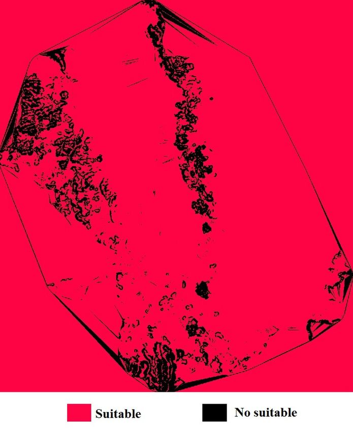
ISPRS Int. J. Geo-Inf. 2016, 5, 235                                                                                      3 of 19
ISPRS Int. J. Geo-Inf. 2016, 5, 235                                                                                      3 of 18

                                           Figure 1. Location of the study area.
                                           Figure 1. Location of the study area.

2.2. Collection and Pre-Processing of the Data
2.2. Collection and Pre-Processing of the Data
      Four scenes covering the study area and taken by the Landsat sensor (Path 32, Row 40) were
      Four scenes covering the study area and taken by the Landsat sensor (Path 32, Row 40) were
used. The spatial resolution of the scenes was 30 m × 30 m. The four scenes corresponded to the years
used. The spatial resolution of the scenes was 30 m × 30 m. The four scenes corresponded to the
1989, 1999, 2009 and 2014 and they were obtained from the United States Geological Survey [41]. The
years 1989, 1999, 2009 and 2014 and they were obtained from the United States Geological Survey [41].
characteristics of each of the scenes are presented in Table 1.
The characteristics of each of the scenes are presented in Table 1.
       Table 1. Characteristics of the scenes corresponding to the urban and peripheral areas of Chihuahua.
      Table 1. Characteristics of the scenes corresponding to the urban and peripheral areas of Chihuahua.
      Satellite        Capture Data                                  Characteristics                               Path/Row
    Landsat (TM)
     Satellite             1989 Data
                       Capture                              7 spectralCharacteristics
                                                                       bands, 30 m resolution                        32/40
                                                                                                                   Path/Row
    Landsat (TM)           1999                             7 spectral bands, 30 m resolution                        32/40
   Landsat (TM)            1989                            7 spectral bands, 30 m resolution                         32/40
    Landsat(TM)
   Landsat  (TM)           2009
                           1999                            77 spectral
                                                              spectral bands,
                                                                       bands, 30
                                                                              30 m
                                                                                 m resolution
                                                                                    resolution                       32/40
                                                                                                                     32/40
   Landsat (TM)
   Landsat  (OLI)          2014
                           2009        8 spectral bands, 307 m  resolution;
                                                              spectral      panchromatic
                                                                       bands,              band, 15 m resolution
                                                                              30 m resolution                        32/40
                                                                                                                     32/40
   Landsat (OLI)            2014       8 spectral bands, 30 m resolution; panchromatic band, 15 m resolution         32/40
       The scenes were radiometrically corrected. The conversion from digital numbers (DN´s) to
 reflectance values
       The scenes    wasradiometrically
                  were    performed withcorrected.
                                            the Top of   theconversion
                                                       The   Atmosphere    (TOA)
                                                                        from       process,
                                                                              digital       which
                                                                                      numbers      allows
                                                                                                (DN´s)  to
 making   comparisons    among    images  from   different  dates.  The radiometric   conversion
 reflectance values was performed with the Top of the Atmosphere (TOA) process, which allows      for  the
 Landsat  TM sensor was
 making comparisons        performed
                       among   images by  following
                                       from  differentEquations
                                                       dates. The(1) and (2), where
                                                                   radiometric      the spectral
                                                                               conversion for theradiance
                                                                                                  Landsat
(TM) sensor
      and thewas
              TOA  reflectance  (  ) were obtained:
                 performed by following Equations (1) and (2), where the spectral radiance (L ) and the             λ
           = (( (ρλ ) were
TOA reflectance        − obtained:
                              )/(                         −              )) ∗ (        −              )+                     (1)

       Lλ = (( Lmaxλ − Lminλ ) / ( QCALmax − QCALmin∗ ∗        )) ∗ ( QCAL − QCALmin) + Lminλ       (1)
                                             =                                                   (2)
                                                       ∗
                                                  π ∗ L λ ∗ d2
where          is DN;               and ρλ = ESUNare        the minimum and maximum quantized
                                                      λ ∗ cosθs
                                                                                                    (2)
calibrated pixel value, respectively;        is the spectral radiance scales to        ;        is the
where QCAL is DN; QCALmin and QCALmax are the minimum and maximum quantized calibrated
spectral radiance scales to           ; is the distance from the earth to the sun;       is the mean
pixel value, respectively; Lminλ is the spectral radiance scales to QCALmin; Lmaxλ is the spectral
solar exoatmospheric irradiance; and      is the solar zenith angle.
radiance scales to QCALmax; d is the distance from the earth to the sun; ESUNλ is the mean solar
     In the case of the data from the Landsat OLI, the radiometric conversion was performed
exoatmospheric irradiance; and θs is the solar zenith angle.
applying Equation (3).
                                                                    ´
                                                          ∗
                                                              =                                                              (3)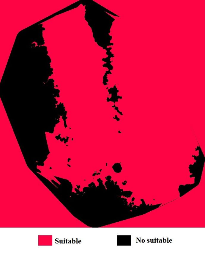
ISPRS Int. J. Geo-Inf. 2016, 5, 235                                                                            4 of 19

    In the case of the data from the Landsat OLI, the radiometric conversion was performed applying
Equation (3).
                                                     ρλ
                                             ρ∗λ =                                               (3)
                                                   sinθSE
where ρλ is the TOA planetary reflectance, with a correction for the solar angle, and θSE is the local
sun elevation angle.
     For the reflectance normalization of the images from 1989, 1999 and 2009, the image from Landsat
OLI was used. This process allowed an improvement on the histograms by modifying the brightness
values in the images from 1989, 1999 and 2009, taking as a reference the image from 2014. With this,
spectral variations of the land use covers were minimized [42].
     As a final step for data processing, the scenes were edited and the study area was defined on the
images by using the software ArcMap 10.2® . The edges were made similar to those of the watersheds of
the area. Such edges were taken from the digital elevation model of the state of Chihuahua. All scenes
were ensured to cover the same area after the edition process.

2.3. Land Use Classification
     Image layer stacking was performed with the software ERDAS® . This procedure allowed
generating false/true colored images, which were required for the analysis of land use classification.
For the case of the Landsat TM sensor, band 5 corresponding to the infrared channel (1.55–1.75 µm),
band 4 in the near infrared range (0.76–0.90 µm), and the band 3 in the red range (0.63–0.69 µm) were
used. These combinations were made based on the recommendations by Lillesand and Kiefer [43]
and applied to the images from the years 1989, 1999 and 2009. Likewise, band 6 corresponding to the
medium infrared channel (1.57–1.65 µm), band 5 in the near infrared range (0.85–0.88 µm), and band 4
in the red range (0.64–0.67 µm) were used for the Landsat OLI. These combinations were applied to
the image from the year 2014.
     A classification based on the method of maximum likelihood was applied to obtain the information
of land use (Equation (4)). This method employed Gaussian probability. As a result, thematic maps
of land use were obtained for each year indicated in the second column of Table 1. The classification
areas included the following land use types: (1) Croplands; (2) Human settlements; (3) Shrublands;
(4) Grasslands; (5) Oak forest; (6) Water bodies; and (7) Riparian vegetation. The image carries
properties allusive to each type of land use as shown in Table 2.

                                                    1               1                 −1
                         gi ( x ) = In p (ωi ) −
                                                    2
                                                      In   ∑i   −
                                                                    2
                                                                      ( x − mi ) T ∑ i ( x − mi )                 (4)

where gi is the class, x represents the n-dimensional data (where n is the number of bands), p (ωi ) is
the probability that the class ωi appears in the image and that is assumed for all classes, |∑i| is the
determinant of the co-variance matrix with data from class ωi , T is the transposed matrix, ∑i−1 is the
inverse matrix and mi is the vector.

        Table 2. Definition of land uses for the study area and properties of corresponding training areas.

           Land Use                            Properties of the Training Areas from Each Land Use Type
         Croplands                    Irregular shape composed of pixels colored “Peridot Green” and “Ultramarine”
     Human settlements                           Irregular shape composed of pixels colored “Glacier Blue”
         Shrubland                                 Irregular shape composed of pixels colored “Lime Dust”
         Grasslands                               Irregular shape composed of pixels colored “Cantaloupe”
         Oak forest                               Irregular shape composed of pixels colored “Green Leaf”
        Water bodies                              Irregular shape composed of pixels colored “Dark Navy”
     Riparian vegetation                        Irregular shape composed of pixels colored “Quetzal Green”
ISPRS Int. J. Geo-Inf. 2016, 5, 235 5 of 19
2.4. Land Use Classification Accuracy
The cartography of land use land cover from the government of the state of Chihuahua
(scale 1:50,000) was used for accuracy validation [44]. The cartography corresponding to land use land
cover from the Mexican Institute of Statistics, Geography and Informatics (INEGI) (scale 1:250,000) was
also employed [40]. In addition, data from field sampling and photointerpretation were considered
during the validation process.
The statistical index KAPPA [45] was used to determine the accuracy of the land use classification
on the maps. KAPPA is a discrete multivariate technique for comparing classes through a matrix [46].
It can be used to establish the degree of similarity between mapped and actual or real values of land
use [47]. A KAPPA value equal to one indicates a 100% similarity between mapped and real values.
Conversely, a value equal to zero suggests a similarity of 0%. KAPPA is represented by Equation (5).
N ∑K Xii ∑k ( Xi+ ∗ X+i )
K APPA = (5)
N 2 − ∑ k ( Xi + ∗ X + i )
where KAPPA is the Kappa index; k is the total number of matrix rows; Xii is the observation number
on row i and column i (along the diagonal); Xi+ and X+i are total marginal for row i and column i,
respectively; and N is the total number of observations.
To estimate the KAPPA index, a group of sample points in the peripheral area was employed.
The resulting accuracy is shown in Table 3.
Table 3. Accuracy of the land use classification.
Precision
Land Use
1989 1999 2009 2014
Croplands 0.82 1.00 1.00 1.00
Human settlements 1.00 1.00 0.83 1.00
Shrublands 0.61 0.85 0.57 0.44
Grasslands 0.83 0.80 1.00 0.51
Oak forest 0.87 1.00 1.00 1.00
Water bodies 1.00 1.00 1.00 1.00
Riparian vegetation 1.00 1.00 1.00 0.81
General Precision KAPPA 0.87 0.95 0.91 0.82
2.5. Models of Markov Chains and Cellular Automata
To elaborate projections of land use change for future years, the geosimulation techniques of
MC and CA were employed [48]. They account for the changes in land use between two dates by
extrapolating them assuming constant changes [49]. The CA technique includes a simulation model
where space and time are discrete variables while the assigned interactions are local variables [30]. It is
fed with the results from the MC methodology to simulate land use in a future time. In this study,
the classifications of 1989 and 1999 were used to estimate the land uses of 2009. Likewise, the land
uses of 2014 were estimated based on the classifications of 1999 and 2009.
The MC methodology was implemented in the MARKOV module of the software Idrisi Selva® .
This technique is based on a stochastic model that describes the probability of change from one state to
another through a transition probability matrix [28]. The results of the MC methodology include a
probability matrix, a matrix of transition areas and transition probability maps. The probability matrix
includes the probability of one land use to change from one category to another. This matrix is the
result of the crossing between the images after setting a proportional error. The matrix of transition
areas states the number of pixels that are expected to change from each land use to the others during
the period of time analyzed. The transition probability maps are generated based on the projections of
possible changes during the period analyzed. In this study, changes in land uses of 1989, 1999, 2009ISPRS Int. J. Geo-Inf. 2016, 5, 235 6 of 19
and 2014 were used to develop the transition probability matrix that helped to develop the land use
projections for 2019 and 2024. The mathematical expression of the transition probability is:
m
∑ Pij = 1 i = 1, 2 . . . ...m (6)
I =1
P11 P12 . . . P1m
P = ( Pij) = P21 P12 P2m (7)
Pm1 Pn2 Pmm
ISPRS Int. J. Geo-Inf. 2016, 5, 235 6 of 18
where Pij is the the probability of transition from one land use to another, and m is the total number of
where
land Pijtypes
use is theofthe
theprobability
study area.ofPij
transition from
values stay one land
within use to0–1.
the range another, and m is the total number
of land
According to the non-after effect of the Markov methodology0–1.
use types of the study area. Pij values stay within the range and the condition equations of
Bayes,According
the Markov to prediction
the non-after
modeleffect of the Markov
is obtained methodology
(Equation 8): and the condition equations of
Bayes, the Markov prediction model is obtained (Equation 8):
= P(n−1) Pij
P ((n)) = (8)
( ) (8)
whereP ((n))isisthe
where probabilityP inintime
theprobability timen, (,n (− 1−) 1)is the probability
is the probability of the previous
of the previous time n. .
time
The
The combination
combinationofof MCMC andand CA wasCA implemented
was implemented through the module
through the of CA_Markov
module available
of CA_Markov
in the software ® , which allows
available in theIDRISI
softwareSelva
IDRISI Selva®, which simulating
allows the dynamics
simulating theofdynamics
growth based on thebased
of growth increase
on
of the number of pixels. Each pixel can take a value from a finite set of
the increase of the number of pixels. Each pixel can take a value from a finite set of states [34]. All states [34]. All pixels are
affected
pixels are byaffected
a transition function that
by a transition takesthat
function as arguments the measured
takes as arguments values ofvalues
the measured the pixels
of the and the
pixels
values
and the of values
the neighboring pixels as a pixels
of the neighboring function asof a time. Cellular
function Automata
of time. Cellular and MC wereand
Automata implemented
MC were
to simulate thetoland
implemented uses of
simulate the2009land and 2014.
uses Sinceand
of 2009 this2014.
period comprehends
Since this period five years, periods
comprehends five of the
years,
same
periodsnumber
of theofsameyears were used
number to estimate
of years were used landtouses of the land
estimate future. That
uses is, land
of the uses
future. were
That is,simulated
land uses
for thesimulated
were years 2019for and
the2024.
years 2019 and 2024.
For
Forthethesimulations,
simulations,it was
it was assumed
assumed thatthatthe probabilities
the probabilitiesof change were low
of change were and constant
low during
and constant
the periods
during the analyzed. Thus, theThus,
periods analyzed. transition probability
the transition matrix created
probability matrixfrom the changes
created from theobservedchanges
between
observed2009 and 2014
between 2009wasandused
2014towas simulate
used to the land uses
simulate theofland
2019. Likewise,
uses of 2019.the transition
Likewise, theprobability
transition
matrix of 2014
probability and 2019
matrix of 2014wasandused2019 to was
estimate
usedthe land usesthe
to estimate of land
2024.uses of 2024.
In
In an
aniterative
iterativeprocess,
process,thethemodule
module ofofCA_Markov
CA_Markov uses
usesthethe
transition
transitionprobability of each
probability landland
of each use
to establish
use to establishthe susceptibility
the susceptibility of each pixel,
of each based
pixel, on their
based properties,
on their to betooccupied
properties, be occupiedby each of the
by each of
other typestypes
the other of land use. While
of land use. Whilethat isthat
performed,
is performed,a spatial filter restricts
a spatial the susceptibility
filter restricts of pixels
the susceptibility of
located away from
pixels located away thefrom
classthe
being processed,
class which is done
being processed, whichbyisassigning
done by aassigning
value of greater
a valuepreference
of greater
to neighboring
preference areas. In thisareas.
to neighboring study, Inspatial
this study, of 5 ×filters
filtersspatial 5 were ofapplied
5 × 5 were(Figure
applied2). (Figure 2).
0 0 1 0 0
0 1 1 1 0
1 1 1 1 1
0 1 1 1 0
0 0 1 0 0
Figure2.2.The
Figure The55×
× 55 filter
filter configuration
configuration used
used in CA_Markov.
in CA_Markov.
2.6. Suitability
2.6. Suitability Parameters
Parameters and
and Limitations
Limitations for
for Urban
Urban Growth
Growth
The parameters
The parameters to
to define
define the
the suitability
suitability of
of aa given
given pixel
pixel to
to change
change from
from one
one type
type of
of land
land use
use to
to
anotherwere
another weredefined.
defined. Such
Such parameters
parameters serveserve to represent
to represent the susceptibility
the susceptibility of the
of the land to beland to be
occupied
occupied by each of the other land uses. These parameters were assigned to the variables
by each of the other land uses. These parameters were assigned to the variables of elevation, slope, of
elevation, slope, distance to rivers and distance to roads. It was assumed that these variables
remained unchanged over the 25 years represented by the dates of the oldest and most recent
satellite images analyzed in this study. The suitability parameters for the variables of elevation and
slope were defined as zero for not suitable and one for suitable (Figure 3). The suitability parameters
for distance to rivers and distance to roads were assigned on a scale of 0 to 255 to represent aISPRS Int. J. Geo-Inf. 2016, 5, 235 7 of 19
distance to rivers and distance to roads. It was assumed that these variables remained unchanged over
the 25 years represented by the dates of the oldest and most recent satellite images analyzed in this
study. The suitability parameters for the variables of elevation and slope were defined as zero for not
suitable and one for suitable (Figure 3). The suitability parameters for distance to rivers and distance
to roads were assigned on a scale of 0 to 255 to represent a minimum and maximum convenience,
respectively
ISPRS (Figure
Int. J. Geo-Inf. 2016,4).
5, 235 7 of 18
ISPRS Int. J. Geo-Inf. 2016, 5, 235 7 of 18
Figure
Figure 3.
3. Suitability
Suitabilityparameters:
parameters:(left) Red
(left) Cells
Red areare
Cells suitable elevations
suitable for urban
elevations development,
for urban and
development,
Figure 3. Suitability parameters: (left) Red Cells are suitable elevations for urban development, and
Black Cells are elevations not suitable for urban development; and (right) Red Cells
and Black Cells are elevations not suitable for urban development; and (right) Red Cells are are slopes
Black Cells are elevations not suitable for urban development; and (right) Red Cells are slopes
suitable for urban development, and Black Cells are slopes
slopes not
not suitable
suitable for
for urban
urban development.
development.
suitable for urban development, and Black Cells are slopes not suitable for urban development.
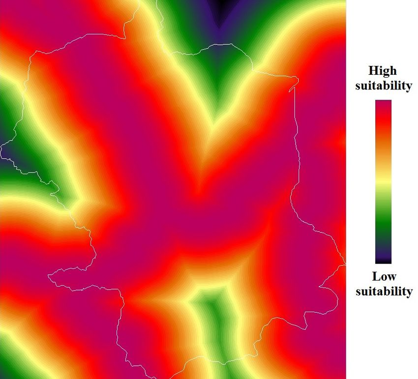
Figure 4. Suitability parameters: (left) distance to rivers (m); and (right) distance to roads (m).
Figure 4. Suitability parameters: (left) distance to rivers (m); and (right) distance to roads (m).
Figure 4. Suitability parameters: (left) distance to rivers (m); and (right) distance to roads (m).
2.7. Validation of the Land Use Change Projections
2.7. Validation of the Land Use Change Projections
2.7. Validation of the Land
The transition Use Change
probability Projections
matrix, matrix of transition areas and transition maps for 1989 and
The transition probability matrix, matrix of transition areas and transition maps for 1989 and
1999 The
were created probability
transition with the Markov
matrix, methodology. Then,areas
matrix of transition we used the CA_Markov
and transition maps formodule
1989 and to
1999 were created with the Markov methodology. Then, we used the CA_Markov module to
simulate
1999 werethe land with
created use ofthe2009. Likewise,
Markov the transition
methodology. probability
Then, we matrix, the matrix
used the CA_Markov moduleoftotransition
simulate
simulate the land use of 2009. Likewise, the transition probability matrix, the matrix of transition
area and use
the land the transition maps of 1999
of 2009. Likewise, and 2009 were
the transition generated
probability and the
matrix, thenmatrix
used to
ofsimulate
transitionthearea
change
and
area and the transition maps of 1999 and 2009 were generated and then used to simulate the change
in land use for 2014.
the transition maps of 1999 and 2009 were generated and then used to simulate the change in land
in land use for 2014.
The
use for validation of the model to simulate land use change was conducted by comparing the
2014.
The validation of the model to simulate land use change was conducted by comparing the
results
Theofvalidation
the estimated land to
of the model use changes
simulate landwith the land
use change wasuses verified
conducted through supervised
by comparing the results
results of the estimated land use changes with the land uses verified through supervised
classifications for 2009 and 2014. For this, a randomly stratified sampling design
of the estimated land use changes with the land uses verified through supervised classificationswas used and the
for
classifications for 2009 and 2014. For this, a randomly stratified sampling design was used and the
K
2009 index
APPA and wasFor
2014. employed. Once the simulated
this, a randomly land uses design
stratified sampling were validated,
was usedestimations of land
and the KAPPA usewas
index for
KAPPA index was employed. Once the simulated land uses were validated, estimations of land use for
2019 and 2024
employed. Oncewere
themade. Finally,
simulated theuses
land procedure used in this
were validated, study is summarized
estimations in Figure
of land use for 2019 and 5. 2024
2019 and 2024 were made. Finally, the procedure used in this study is summarized in Figure 5.
were made. Finally, the procedure used in this study is summarized in Figure 5.ISPRS Int. J. Geo-Inf. 2016, 5, 235 8 of 19
ISPRS Int. J. Geo-Inf. 2016, 5, 235 8 of 18
Figure 5. Procedure followed to analyze the spatio-temporal changes of seven land uses in the urban
Figure 5. Procedure followed to analyze the spatio-temporal changes of seven land uses in the urban
and metropolitan areas of Chihuahua City.
and metropolitan areas of Chihuahua City.
3. Results
3. Results
3.1. Detection of Land Use Changes
3.1. Detection of Land Use Changes
Results from the analysis of land use show a remarkable gain for the surface area corresponding
Results from the analysis of land use show a remarkable gain for the surface area corresponding
to Human settlements (Table 4). Chihuahua City increased more than twice its occupied area in the
to Human settlements (Table 4). Chihuahua City increased more than twice its occupied area in the
past 25 years. The expansion occurred mainly to the north and southeast directions (Figure 6). In
past 25 years. The expansion occurred mainly to the north and southeast directions (Figure 6). In these
these directions, the lowest elevations exist and this condition makes the terrain desirable for
directions, the lowest elevations exist and this condition makes the terrain desirable for residential
residential development. Of the categories analyzed, the only one that showed continuous growth is
development. Of the categories
the Human settlements, with analyzed, the only
13.57%, 17.01%, one that
24.63% andshowed
28.50%continuous growth
for 1989, 1999, 2009is the
andHuman
2014,
settlements, with 13.57%, 17.01%, 24.63% and 28.50% for 1989, 1999, 2009 and 2014,
respectively. In contrast, the land uses of Shrublands and Grasslands showed a reduction in their respectively.
Inarea
contrast,
duringthe
theland
sameuses of Shrublands
period and Grasslands
(Figure 7). Regarding showed
the classes a reduction
of Croplands, in their
Oak forest,area during
Water the
bodies
same period (Figure 7). Regarding the classes of Croplands, Oak forest, Water bodies
and Riparian vegetation, their occupied surface areas stayed in general constant. Each of these and Riparian
vegetation, their occupied
classes presented a changesurface areas1%
lower than stayed in period
for the general1989–2014.
constant. Each of these classes presented a
change lower than 1% for the period 1989–2014.ISPRS Int. J. Geo-Inf. 2016, 5, 235 9 of 19
ISPRS Int. J. Geo-Inf. 2016, 5, 235 9 of 18
Table 4. Occupation
Table percentages
4. Occupation of seven
percentages land use
of seven types
land use in the urban
types in theand peripheral
urban areas of Chihuahua
and peripheral areas of
City in 1989, 1999,
Chihuahua City 2009 and1999,
in 1989, 2014.
2009 and 2014.
Occupation (%)
Land Use Occupation (%)
Land Use 1989 1999 2009 2014
1989 1999 2009 2014
Croplands 4.12 3.76 3.66 3.48
Croplands
Human settlements 4.12
13.57 3.76
17.01 3.66
24.63 3.48
28.58
Human settlements 13.57 17.01 24.63 28.58
Shrublands
Shrublands 54.53
54.53 53.64
53.64 49.35
49.35 48.06
48.06
Grasslands
Grasslands 23.50
23.50 21.67
21.67 18.18
18.18 16.01
16.01
Oakforest
Oak forest 2.89
2.89 2.86
2.86 2.86
2.86 2.86
2.86
Water bodies
Water bodies 0.07
0.07 0.08
0.08 0.11
0.11 0.11
0.11
Riparian vegetation 1.31 0.97 1.21 0.90
Riparian vegetation 1.31 0.97 1.21 0.90
Figure 6. Land use maps of the city of Chihuahua for the years 1989, 1999, 2009 and 2014.
Figure 6. Land use maps of the city of Chihuahua for the years 1989, 1999, 2009 and 2014.ISPRS Int. J. Geo-Inf. 2016, 5, 235 10 of 19
ISPRS Int. J. Geo-Inf. 2016, 5, 235 10 of 18
50
1989 1999 2009 2014
40
Surface (ha × 1000)
30
20
10
0
CL HS OF WB S G R
Land use
Figure 7. Growth dynamics of seven land use types in the urban and peripheral areas of Chihuahua
Figure 7. Growth dynamics of seven land use types in the urban and peripheral areas of Chihuahua
City during 1989–2014. CL, Croplands; HS, Human settlements; OF, Oak forest; WB, Water bodies; S,
City during 1989–2014. CL, Croplands; HS, Human settlements; OF, Oak forest; WB, Water bodies;
Shrublands; G, Grasslands;
S, Shrublands; R, Riparian
G, Grasslands; vegetation.
R, Riparian vegetation.
The dynamics of land use changes are presented in Table 5. The Grasslands presented the
Theloss
greatest dynamics of land
of surface withuse changes
1,471 are presented
ha during in 1989–1999.
the period Table 5. TheThis
Grasslands
land usepresented
increasedtheitsgreatest
loss in
loss of surface with 1471 ha during the period 1989–1999. This land use increased its
surface to 2,820 ha during the period 1999–2009 and further reduced its area to 1,746 ha during the loss in surface
to 28202009–2014.
period ha duringThethe area
period 1999–2009
occupied and furtherwas,
by Shrublands reduced its area
after the to 1746 the
Grasslands, ha during
category the period
that lost
2009–2014. The area occupied by Shrublands was, after the Grasslands, the category
most of the surface area. By contrast, the Human settlements experienced the largest growth with that lost most
a
of the surface area. By contrast, the Human settlements experienced the largest growth
total increase of 12,097 ha for the period of 1989–2014. The location of housing projects has markedly with a total
increase of to
contributed 12,097 ha for the
the increase period
in the area of 1989–2014.
occupied The location
by Human of housing projects has markedly
settlements.
contributed to the increase in the area occupied by Human settlements.
Table 5. Change dynamics of seven types of land use in the urban and peripheral areas of Chihuahua
Table 5. Change dynamics of seven types of land use in the urban and peripheral areas of Chihuahua
City. Positive and negative numbers indicate gains and losses of surface, respectively.
City. Positive and negative numbers indicate gains and losses of surface, respectively.
Category Surface (ha)
Total
Category
Year 1989–1999 Surface
1999–2009(ha) 2009–2014
Total
Croplands
Year −290
1989–1999 −82
1999–2009 −146
2009–2014 −518
Human settlements
Croplands 2,772
−290 6,143
−82 3,182
−146 12,097
−518
Shrublands
Human settlements −26
2772 0
6143 0
3182 −26
12,097
Shrublands
Grasslands −12
26 0
21 00 33 −26
Grasslands
Oak forest 12
−720 21
−3,458 0
−1,041 −5,21933
Oak forest −720 −3458 −1041 −5219
Water
Water bodies
bodies −1,471
− 1471 −2,820
−2820 −1,746
−1746 −6,037
−6037
Riparian
Riparian vegetation
vegetation −−273
273 195
195 −249
−249 −327
−327
The transition probabilities of the land use corresponding to the periods 1989–1999, 1999–2009,
The transition probabilities of the land use corresponding to the periods 1989–1999, 1999–2009,
and 2009–2014 are shown in Table 6. Bold numbers along the diagonal show the transition
and 2009–2014 are shown in Table 6. Bold numbers along the diagonal show the transition probabilities
probabilities among the study periods. The probability of change from the land use of agriculture to
among the study periods. The probability of change from the land use of agriculture to the one
the one of Human settlements was 16% for the period 1999–2009 and decreased to 14% during
of Human settlements was 16% for the period 1999–2009 and decreased to 14% during 2009–2014.
2009–2014. Shrublands had a probability of change of 11% during 1989–1999, 15% during 1999–2009
Shrublands had a probability of change of 11% during 1989–1999, 15% during 1999–2009 and 12%
and 12% during 2009–2014. Moreover, Grasslands presented the highest increase in the probability
during 2009–2014. Moreover, Grasslands presented the highest increase in the probability of change
of change during the same period: 16% for the period 1989–1999, 23% for the period 1999–2009 and
during the same period: 16% for the period 1989–1999, 23% for the period 1999–2009 and 20% for the
20% for the period 2009–2014.
period 2009–2014.
This transition probability matrix (Table 6) indicates that the classes of Croplands, Shrublands,
This transition probability matrix (Table 6) indicates that the classes of Croplands, Shrublands,
Oak forest, Water bodies and Human settlements had been stable with a tendency to stay in the
Oak forest, Water bodies and Human settlements had been stable with a tendency to stay in the same
same land use during the periods 1989–1999 to 2009–2014, as indicated by the probabilities close to
land use during the periods 1989–1999 to 2009–2014, as indicated by the probabilities close to 1.0 in the
1.0 in the transition matrix. Regarding Grasslands, there was a decrease in the transition probability
transition matrix. Regarding Grasslands, there was a decrease in the transition probability of 0.82 from
of 0.82 from the period of 1989–1999 to 0.75 during 1999–2009 and to 0.79 for the period 2009–2014.
The decrease in the transition probability indicates an increased likelihood for change of the
Grasslands to another type of land use.ISPRS Int. J. Geo-Inf. 2016, 5, 235 11 of 19
ISPRS Int. J. Geo-Inf. 2016, 5, 235 11 of 18
the period of 1989–1999 to 0.75 during 1999–2009 and to 0.79 for the period 2009–2014. The decrease in
Tableprobability
the transition 6. Transitionindicates
probability
anmatrix for the
increased periods 1989–1999,
likelihood 1999–2009,
for change and 2009–2014.
of the Grasslands to another
typeLand
of land
Useuse. Year CL HS S G OF WB R
1989–1999 0.81 0.05 0.13 0.00 0.00 0.00 0.00
Table 6. Transition probability matrix for the periods 1989–1999, 1999–2009, and 2009–2014.
CL 1999–2009 0.83 0.16 0.00 0.00 0.00 0.00 0.00
Land Use
2009–2014
Year
0.85
CL HS
0.14 S
0.00 G 0.00
OF
0.00
WB R
0.00 0.00
1989–1999 0.00 0.89 0.10 0.00 0.00 0.00 0.00
1989–1999 0.81 0.05 0.13 0.00 0.00 0.00 0.00
HS CL
1999–2009
1999–2009 0.00
0.83 0.160.89 0.00 0.100.00 0.00
0.00 0.00
0.00 0.00
0.00 0.00
2009–2014
2009–2014 0.01
0.85 0.140.90 0.00 0.010.00 0.01
0.00 0.01
0.00 0.01
0.00 0.01
1989–1999
1989–1999 0.00
0.00 0.890.11 0.10 0.870.00 0.00
0.00 0.00
0.00 0.00
0.00 0.00
S HS 1999–2009
1999–2009 0.00
0.00 0.890.15 0.10 0.820.00 0.00
0.00 0.00
0.00 0.00
0.00 0.01
2009–2014
2009–2014 0.01
0.00 0.900.12 0.01 0.870.01 0.01
0.00 0.01
0.00 0.01
0.00 0.00
1989–1999
1989–1999 0.00
0.00 0.110.16 0.87 0.000.00 0.82
0.00 0.00
0.00 0.00
0.00 0.00
G S 1999–2009
1999–2009 0.00
0.00 0.150.23 0.82 0.010.00 0.00
0.75 0.00
0.00 0.01
0.00 0.00
2009–2014 0.00 0.12
2009–2014 0.00 0.20 0.87
0.000.00 0.00
0.79 0.00
0.00 0.00
0.00 0.00
1989–1999
1989–1999 0.00
0.00 0.160.00 0.00 0.110.82 0.00
0.00 0.00
0.88 0.00
0.00 0.00
G 1999–2009 0.00 0.23 0.01 0.75 0.00 0.00 0.00
OF 1999–2009 0.01 0.01 0.01 0.01 0.90 0.01 0.01
2009–2014 0.00 0.20 0.00 0.79 0.00 0.00 0.00
2009–2014 0.01 0.01 0.01 0.01 0.90 0.01 0.01
1989–1999 0.00 0.00 0.11 0.00 0.88 0.00 0.00
1989–1999
1999–2009
0.01
0.01 0.01
0.01 0.01
0.010.01 0.01
0.90
0.01
0.01
0.90
0.01
0.01
OF
WB 1999–2009
2009–2014 0.01
0.01 0.010.01 0.01 0.010.01 0.01
0.90 0.01
0.01 0.90
0.01 0.01
2009–2014
1989–1999
0.01
0.01 0.01
0.01 0.01
0.010.01 0.01
0.01
0.01
0.90
0.90
0.01
0.01
WB 1989–1999
1999–2009 0.02
0.01 0.010.00 0.01 0.290.01 0.00
0.01 0.00
0.90 0.01
0.01 0.66
R 1999–2009
2009–2014 0.00
0.01 0.010.16 0.01 0.000.01 0.00
0.01 0.00
0.90 0.00
0.01 0.83
2009–2014
1989–1999 0.29 0.01
0.02 0.000.01 0.010.00 0.01
0.00 0.01
0.01 0.01
0.66 0.90
R
CL, Croplands; HS, 1999–2009 0.00
Human settlements; 0.16 Oak 0.00
OF, 0.00 Water
forest; WB, 0.00bodies;
0.00S, Shrublands;
0.83 G,
2009–2014
Grasslands; R, Riparian vegetation. 0.01 0.01 0.01 0.01 0.01 0.01 0.90
CL, Croplands; HS, Human settlements; OF, Oak forest; WB, Water bodies; S, Shrublands; G, Grasslands;
The algorithm
R, Riparian of CA_Markov determines the exact location of the changes. Thus, the
vegetation.
probability of change of any pixeldetermines
The algorithm of CA_Markov depends on thethe previously
exact location assigned filter and
of the changes. onthe
Thus, theprobability
restriction
ofand suitability
change parameters
of any pixel depends applied to neighboring
on the previously pixels.
assigned filterThe
and Human settlements
on the restriction andshowed an
suitability
increase in the transition probability, indicating a stabilization of this class due to population
parameters applied to neighboring pixels. The Human settlements showed an increase in the transition growth
[40], as shown
probability, in Figure
indicating 8.
a stabilization of this class due to population growth [40], as shown in Figure 8.
24
22 y = 0.0359x - 9.0025
Surface (ha × 1000)
20 R² = 0.9606
18
16
14
12
10
500 600 700 800 900
Population ( × 1000)
Figure8.8.Relationship
Figure Relationshipbetween
betweenthe
theurban
urbansprawl
sprawland
andits
itspopulation.
population.
Theprevious
The previousresults
resultsindicate
indicatethree
threemainmainfindings
findingsfrom
fromthe
theanalysis
analysisof
ofthe
thegrowth
growthdynamics
dynamicsof of
Chihuahua City: (1) the class that had the greatest loss of land use and the one that had the
Chihuahua City: (1) the class that had the greatest loss of land use and the one that had the greatest greatest
transitionchange
transition changewaswas Grasslands;
Grasslands; (2)(2)
it isitexpected
is expected
that that Croplands
Croplands continue
continue to change
to change to areas;
to urban urban
areas; and (3) Shrublands are another type of land use that will increase its probability of change to
urban area (Table 6). This shows a dominance of the urban land use over the Croplands, GrasslandsISPRS Int. J. Geo-Inf. 2016, 5, 235 12 of 19
and
ISPRS(3)
Int.Shrublands
J. Geo-Inf. 2016,are another type of land use that will increase its probability of change to urban
5, 235 12 of 18
area (Table 6). This shows a dominance of the urban land use over the Croplands, Grasslands and
Shrublands.
and Shrublands. In addition, this indicates
In addition, a continuous
this indicates changechange
a continuous and a pressure on the neighboring
and a pressure natural
on the neighboring
resources due to the
natural resources due expansion of the urban
to the expansion of thearea through
urban time. time.
area through
3.2. Validation of
3.2. Validation of the
the Land
Land Use
Use Change
Change Projections
Projections
For
For the
the validation
validation of
of land
land use
use change
change projections,
projections, the
the land
land uses
uses of
of 2009
2009 and
and 2014 were simulated
2014 were simulated
with
with CA_Markov. The simulated land uses were then compared with the actual land uses resulting
CA_Markov. The simulated land uses were then compared with the actual land uses resulting
from
from the
the supervised
supervised classifications
classifications of
of the
the same
same years.
years. The
The comparison
comparison ofof simulated
simulated and
and actual
actual values
values
of land use are shown in Figure 9, where deviations can be visually assessed.
of land use are shown in Figure 9, where deviations can be visually assessed.
45 45
40 2009 S-2009 40 2014 S-2014
35
Surface (ha × 1000)
35
Surface (ha × 1000)
30 30
25 25
20 20
15 15
10 10
5 5
0 0
CL HS S G OF WB R CL HS S G OF WB R
Land use Land use
Figure 9.9.Comparison
Figure Comparisonof of simulated
simulated and and real uses
real land landfor:
uses for:
2009 2009and
(left); (left);
2014 and 2014
(right). CL,(right). CL,
Croplands;
Croplands; HS, Human settlements; OF, Oak forest; WB, Water bodies; S, Shrublands;
HS, Human settlements; OF, Oak forest; WB, Water bodies; S, Shrublands; G, Grasslands; G, Grasslands;
R, Riparian
R, Riparian vegetation.
vegetation.
It can be observed in Figure 9 that for both, 2009 and 2014, the differences between the actual
It can be observed in Figure 9 that for both, 2009 and 2014, the differences between the actual and
and simulated land uses were small. The overall accuracy was 90% for 2009 and 91% for 2014. The
simulated land uses were small. The overall accuracy was 90% for 2009 and 91% for 2014. The greatest
greatest accuracy was obtained for the class of Oak forest, while the class that showed the lowest
accuracy was obtained for the class of Oak forest, while the class that showed the lowest accuracy was
accuracy was Human settlements with 0.79 and 0.70 for 2009 and 2014, respectively (Table 7).
Human settlements with 0.79 and 0.70 for 2009 and 2014, respectively (Table 7).
The 100% agreement between the simulated and real values for the class of Oak forest were
obtained because the probability of change of this class was unaffected by other classes. In addition,
Table 7. Agreement between the real and simulated values of seven land uses of 2009 and 2014 in the
this urban
class is not geographically close to the urban area. In the case of Human settlements, the
and peripheral areas of Chihuahua City.
resulting lower agreement could be due to the growth patterns influenced by different causes such
as socio-economic, political, and other larger contextual
Agreement factors.
betweenStill,
Real all
andagreement
Simulated values estimated
Land Use
during the validation process could be considered2009 as very good. The 2014
values of KAPPA close to 1.0
indicate a high similarity between the simulated and real values, as well as a spatial distribution of
Croplands 0.88 0.86
the simulated land uses close to reality. Based on 0.79
Human settlements
the above, CA_Markov 0.70
model can be used to
predict future changes inShrublands
land uses in the study area.0.90 0.95
Grasslands 0.85 0.85
Oak forest
Table 7. Agreement between 0.99 of seven land uses
the real and simulated values 0.99
of 2009 and 2014 in the
urban and peripheralWater
areas bodies
of Chihuahua City. 0.99 0.99
Riparian vegetation 0.92 0.99
Agreement between Real and0.91
Simulated
General
Land Use KAPPA
Precision 0.90
2009 2014
Croplands 0.88 0.86
The 100% agreement between the simulated and real values for the class of Oak forest were
Human settlements 0.79 0.70
obtained because the probability of change of this class was unaffected by other classes. In addition, this
Shrublands 0.90 0.95
class is not geographically close to the urban area. In the case of Human settlements, the resulting lower
Grasslands 0.85 0.85
Oak forest 0.99 0.99
Water bodies 0.99 0.99
Riparian vegetation 0.92 0.99
General Precision KAPPA 0.90 0.91ISPRS Int. J. Geo-Inf. 2016, 5, 235 13 of 19
agreement could be due to the growth patterns influenced by different causes such as socio-economic,
political, and other larger contextual factors. Still, all agreement values estimated during the validation
process could be considered as very good. The values of KAPPA close to 1.0 indicate a high similarity
between the simulated and real values, as well as a spatial distribution of the simulated land uses close
to reality. Based on the above, CA_Markov model can be used to predict future changes in land uses in
the study area.
3.3. Simulations of Land Use
The model of CA_Markov was used to simulate the areas occupied by seven land uses for the
years 2019 and 2024, as an effect of the urban development. For the simulation of the land uses of 2019,
the transition probability matrix of the period 2009–2014 was used, setting 2009 as the base year and
considering the following five years of change. Afterwards, the year of 2019 was established as the
starting point to generate the land uses of 2024. For that, the transition probability matrix of the period
2014–2019 was employed.
The transition probabilities for the years 2019 and 2024 are shown in Table 8. The class of
Grasslands, which had the lowest probability represented by a 0.64 in 2014–2019 and 0.58 in 2019–2024,
is the class which would be subjected to the greatest probability of change with a value calculated of
0.79 for 2014 (Table 6) and an estimated and reduced value of 0.58 for the next 10 years (Table 8).
Table 8. Transition probability matrix for 2019 and 2024.
Year CL HS S G OF WB R
2014–2019 0.74 0.25 0.00 0.00 0.00 0.00 0.00
CL
2019–2024 0.68 0.31 0.00 0.00 0.00 0.00 0.00
2014–2019 0.00 0.89 0.10 0.00 0.00 0.00 0.00
HS
2019–2024 0.00 0.89 0.10 0.00 0.00 0.00 0.00
2014–2019 0.01 0.18 0.79 0.00 0.00 0.00 0.00
S
2019–2024 0.01 0.18 0.79 0.00 0.00 0.00 0.00
2014–2019 0.00 0.32 0.02 0.64 0.00 0.00 0.00
G
2019–2024 0.00 0.38 0.03 0.58 0.00 0.00 0.00
2014–2019 0.01 0.01 0.01 0.016 0.90 0.01 0.01
OF
2019–2024 0.01 0.01 0.01 0.01 0.90 0.01 0.01
2014–2019 0.01 0.01 0.01 0.01 0.01 0.90 0.01
WB
2019–2024 0.01 0.01 0.01 0.01 0.01 0.90 0.01
2014–2019 0.01 0.01 0.01 0.01 0.01 0.01 0.90
R
2019–2024 0.01 0.01 0.01 0.01 0.01 0.01 0.90
CL, Croplands; HS, Human settlements; OF, Oak forest; WB, Water bodies; S, Shrublands; G, Grasslands;
R, Riparian vegetation.
It is estimated that Human settlements is the land use that will show the greatest percentage of
change in coverage beginning with 28.57% in 2014 (Table 4) and reaching 38.57% in 2019 (Table 9).
This type of land use will end up covering almost half of the study area (47.33%) in 2024. The classes
of Water bodies, Oak forest and Riparian vegetation will be nearly unaffected by the urban growth.
However, according to the results from the projections for 2019 and 2024, Human settlements will be
extended over adjacent and sensitive areas such as Grasslands and Shrublands (Figure 10).ISPRS Int. J. Geo-Inf. 2016, 5, 235 14 of 19
Table 9. Simulated coverage areas and percentage of occupation of seven land uses of the urban and
peripheral areas of Chihuahua City by 2019 and 2024.
Year 2019 2024
Land Use Surface (ha) Occupation (%) Surface (ha) Occupation (%)
Croplands 2565.23 3.22 2328.43 2.92
Human settlements 30,666.91 38.57 37,636.71 47.33
Shrublands 33,667.13 42.34 30,075.10 37.82
Grasslands 9244.07 11.62 6105.60 7.67
Oak forest 2305.23 2.89 2305.26 2.89
Water bodies 87.02 0.10 86.90 0.10
Riparian vegetation 975.01 1.22 972.73 1.22
Total 79,511 100 79,511 100
ISPRS Int. J. Geo-Inf. 2016, 5, 235 14 of 18
Figure 10.
Figure 10.Simulated
Simulated occupied
occupied areas
areas of seven
of seven landofuses
land uses of theand
the urban urban and peripheral
peripheral areas of
areas of Chihuahua
Chihuahua City by 2019
City by 2019 and 2024. and 2024.
The estimated dynamics of land use gains and losses for the periods 2014–2019 and 2019–2024
The estimated dynamics of land use gains and losses for the periods 2014–2019 and 2019–2024
are shown in Table 10. During these two periods, it is estimated that Shrublands and Grasslands will
are shown in Table 10. During these two periods, it is estimated that Shrublands and Grasslands
suffer the greatest losses of areas. Human settlements, represented by gains of 7,629.92 and 6,969.79
will suffer the greatest losses of areas. Human settlements, represented by gains of 7629.92 and
ha for the periods of 2014–2019 and 2019–2024, respectively, is the class that would experience the
6969.79 ha for the periods of 2014–2019 and 2019–2024, respectively, is the class that would experience
greatest expansion.
the greatest expansion.
Table 10. Dynamics of land use changes for seven land use types of the urban and peripheral areas of
Table 10. Dynamics of land use changes for seven land use types of the urban and peripheral areas of
Chihuahua City by 2019 and 2024.
Chihuahua City by 2019 and 2024.
Year 2014–2019 2019–2024
Year Use
Land 2014–2019
Surface (ha) 2019–2024
Surface (ha)
Croplands
Land Use −241.76
Surface (ha) −236.79(ha)
Surface
Human settlements
Croplands 7,629.91
−241.76 6,969.79
−236.79
Human Shrublands
settlements −5,070.86
7629.91 −3,592.03
6969.79
Shrublands
Grasslands − 5070.86
−3,662.92 − 3592.03
−3,138.47
Grasslands −3662.92 −3138.47
Oak forest −0.76 0.02
Oak forest −0.76 0.02
Water
Water bodies
bodies 0.02
0.02 −0.12
−0.12
Riparian
Riparian vegetation
vegetation 248.01
248.01 −1.27
−1.27
4. Discussion
The model of CA_Markov has been widely used for simulations of land use changes and its
impact on the landscape by projecting possible trends. In this study, the model was used to project
the land uses of the urban and peripheral areas of Chihuahua City by 2019 and 2024. To first
understand the urban growth dynamics, this research determined the land uses of the past years as a
basis for simulating future changes in the study area. This tool is an alternative means of support forISPRS Int. J. Geo-Inf. 2016, 5, 235 15 of 19
4. Discussion
The model of CA_Markov has been widely used for simulations of land use changes and its
impact on the landscape by projecting possible trends. In this study, the model was used to project the
land uses of the urban and peripheral areas of Chihuahua City by 2019 and 2024. To first understand
the urban growth dynamics, this research determined the land uses of the past years as a basis
for simulating future changes in the study area. This tool is an alternative means of support for
urban planners.
Remote sensing produces valuable data with quick acquisition, which can be used for analyses of
land use; for example, the data from the Landsat sensor, which provides images taken from 1972 to
date. This satellite has a worldwide coverage with a medium spatial resolution. The Markov prediction
method employs the historical data from the Landsat sensor to analyze the dynamic behavior of land
use in a time-space pattern. Based on that, forecasts of future changes are estimated.
The methodology employed in this study showed a good level of precision, with values of
the KAPPA index above 0.82. This precision is comparable with the ones estimated in other studies
employing similar methodologies [2]. The high precision in this case was due to a clear spatial
distribution of the land uses in the study area. These land uses are strongly related to the topography
where the City is located. The plain areas are clearly occupied by ecosystems of Grasslands while
surfaces conformed by terrains with slight slopes are dominated by communities of Shrublands.
The results of this study show the feasibility and validity of the CA_Markov based model for simulating
urban land use change.
From 1989 to 2009, the city of Chihuahua grew mainly to the north and southeast directions.
One of the main reasons is the increasing manufacturing industry present in those parts of the city.
In these directions, the lowest elevations exist and these conditions make the terrain desirable for
industrial development. In its growth stage, this industry has been settled on plain lands with access to
the main roads. The most important road in Chihuahua is the one running in the north-south direction,
which connects the city with the rest of the country and with the United States of America. The latter
represents the main market of the manufacturing items produced in the city.
Another reason for this growth could be attributed to the increase on the number of small houses,
which were constructed for people with low incomes. Many of these people work on the manufacturing
industry. Thus, the location of housing projects has markedly contributed to the increase in the area
occupied by Human settlements. Together, these two factors have influenced the city growth dynamics,
the urban structure, its geographical expansion, and the location of the jobs generated in the city.
Before the 1970s, the number of jobs generated by the manufacturing industry was small and their
location was scattered around the city. In those days, jobs were related to mining or logging activities.
This scenario changed with the installation of the industrial parks called “Complejo Industrial
Chihuahua”, “Las Americas” and “Saucito”. Thereafter, Human settlements had a remarkable growth,
with areas where jobs related to the industry sector are concentrated [38]. The location of industrial
parks near the main roads and the houses of social interest are factors that have influenced the growth
of the city, as it can be visually verified on Figure 6. Other factors include the requirement of labor
force, the access to highways, and the proximity of the edge of the urban area to the rural areas.
With the model of CA_Markov the growth of the urban area and the land use change on the
suburban areas were assessed and quantified. Due to the absence of a conservation policy for suburban
land uses, it is expected that a number of both economic and social factors cause alterations on the
land uses of Grasslands, Shrublands and Riparian vegetation areas. The establishment of buffer zones
could improve conditions for the use of land surrounding the city.
Even though the MC and CA methodologies have been criticized for its inability to incorporate
social factors such as human decision [28], this study simulated land use changes for the years of 2009
and 2014 with a high degree of accuracy. One of the reasons for that could be the period between the
dates of the images used, which was in general consistent (10-year period), compared to other studies
that employed only three dates [50] or dates with varied periods among the dates of the images [51].You can also read