SANITY CHECK FOR PERSISTENCE DIAGRAMS
←
→
Page content transcription
If your browser does not render page correctly, please read the page content below
Accepted at the ICLR 2021 Workshop on Geometrical and Topological Representation Learning

S ANITY C HECK FOR P ERSISTENCE D IAGRAMS
 Chen Cai
 Department of Computer Science
 University of California San Diego
 c1cai@ucsd.edu

                                            A BSTRACT

         Recently many efforts have been made to incorporate persistence diagrams, one
         of the major tools in topological data analysis (TDA), into machine learning
         pipelines. To better understand the power and limitation of persistence diagrams,
         we carry out a range of experiments on both graph and shape data, aiming to de-
         couple and inspect the effects of different factors involved. To this end, we propose
         a sanity check for persistence diagrams to delineate critical values and pairings of
         critical values (structure of persistence module). For graph classification tasks,
         we note that while persistence pairing yields consistent improvement over various
         benchmark datasets, it appears that for various filtration functions tested, most dis-
         criminative power comes from critical values. For shape segmentation and clas-
         sification, however, we note that persistence pairing shows significant power on
         most of the benchmark datasets, and improves over summaries based on merely
         critical values. Our results help provide insights on when persistence diagram
         based summaries could be more suitable.

1   I NTRODUCTION

Topological data analysis (TDA) is an emerging field that aims to characterize the shape of low and
high dimensional data via methods stemming from algebraic topology. One of the major tools of
TDA is persistence diagrams (PDs). In recent years, many efforts have been made to utilize PDs
as features for downstream machine learning tasks, such as material science (Buchet et al., 2018),
signal analysis (Perea & Harer, 2015) , cellular data (Cámara, 2017) and shape recognition (Li et al.,
2014). However, the geometry of the PD does not lend itself easily to well-adopted classifiers due
to the lack of Hilbert space structure. To handle this issue, a natural way is to apply vectorization
(Bubenik, 2015; Carrière et al., 2015; Chazal et al., 2014; Kališnik, 2019) or kernelization (Reining-
haus et al., 2015; Carriere et al., 2017) to PDs, i.e., embedding PDs either to a Euclidean space Rd
or a reproducing kernel Hilbert space (RKHS) associated with certain kernels.
However, these approaches still have limitations. First, it has been shown that finite-dimension em-
bedding can miss information about PDs (Carriere & Bauer, 2018). Second, the time of computing
a kernel is quadratic in the number of PDs, which is prohibitive for large-scale applications. Third,
choosing the right vectorization/kernelization and its associated hyper-parameters is not straightfor-
ward and usually requires multiple rounds of trial and error.
Due to these extra complexities, one may wonder whether the benefits of using PDs outweigh the
extra cost. Specifically, PDs have two major components: 1) filtration function and 2) persistence
pairing (decomposition of 1D persistence module). In this paper, we ask a simple yet fundamental
question: How much extra power can persistence pairing bring in?
Our contributions. In this work, we propose a simple sanity check that can shield light on the
power of PDs. Specifically, we permute the persistence points in such a way that only coordinates of
PDs remain the same but the original pairing is completely destroyed. These fake PDs have the same
form as the original PDs and therefore the same kernels for true diagrams can also be applied to fake
ones. We use these fake diagrams as the input for various tasks and check their effectiveness. As we
will see, this simple trick brings various insights on the use of PDs for different problems. To the
best of our knowledge, our paper is the first work systematically quantifying (empirically) the power
of persistence pairing for various applications. Specifically, our contributions are the following.

                                                   1
Accepted at the ICLR 2021 Workshop on Geometrical and Topological Representation Learning
• We propose the sanity check for PDs that decouples the statistics of the critical values of filtration
function and the persistence pairing. Using the proposed method, we find that in graph classifi-
cation, even fake diagrams perform quite well compared to original PDs. As a byproduct of our
extensive experiments, we also provide some rules of thumb for using PDs in graph classification.
• For shape segmentation and classification, we find the power of persistence pairing depends on
the particular featurization chosen. With the right choice of featurization, utilizing persistence
pairing brings in significant improvement. Intuitively, we think that the shape models have more
prominent geometric features in them, which are effectively captured by PDs. In contrast, PDs
seem to be less effective at capturing features for graphs, partly due to the choice of descriptor
functions as well as the nature of noise in graph (random insertions) which makes PDs less stable.
2 E XPERIMENT
Setup. On a high level, we use PDs obtained from different filtration functions as features. Depend-
ing on the task, we choose a proper featurization method followed by SVM for final classification.
We use kernel methods (see D.2) when possible since they tend to perform better, but for large-scale
applications, computing kernels is not feasible so we use vector methods (see D.1). We maintain
the same experiment settings for original PDs and permuted ones (see below). For a comprehen-
sive evaluation, we perform experiments on various tasks (graph classification, shape segmentation,
and object classification) and diverse data types including social networks, molecules/proteins, and
meshes from 3D shapes.
Filtration function. We test degree (deg), Ricci Curvature (Lin et al., 2011) (Ricci), closeness
centrality (cc), and square of Fiedler vector (the eigenvector corresponding to the second smallest
eigenvalue of graph Laplacian, denoted as Fiedler-s) for graph classification. On shape datasets, we
use geodesic distance as filtration function for shape segmentation and closeness centrality for shape
classification. See details about kernels and datasets at appendix A.1.
Sanity check for PDs. We introduce a sanity check that aims to preserve statistics of filtration
function but destroy the persistence pairing of critical values of the filtration function. For a diagram
P = {p1 , p2 , ..., pn } of size n, denote the coordinates of point pi by (xi , yi ) where xi 6= yi for all
i. Take the multiset Pmultiset = {x1 , y1 , x2 , y2 , ..., xn , yn } as input. We then randomly sample two
values, denoted by a and b, without replacement from Pmultiset as the coordinates of the persistence
point in the fake diagram. For diagrams from sublevel filtrations, we ensure all persistence points
in permuted diagrams lie above the diagonal by taking min(a, b) as x-coordiniate and max(a, b) as
y-coordinate of the point in the permuted diagram. Note that it is possible that two birth values can
be paired in fake diagrams. Similar strategy is applied for superlevel filtration as well. Repeat the
same procedure n times and get a fake diagram called Pf ake of size n.
Baseline. As permuting diagrams adds stochasticity in persistence diagrams, we also introduce two
deterministic baselines to better quantify the power of persistence pairing. Pervec (vector obtained
from coordinates of points in the permuted diagram) is a histogram vector of the coordinates of
PD, i.e., the histogram of P . Filvec is a histogram vector of all the filtration function values on
the graph. The length of Pervec and Filvec is a hyper-parameter chosen from {100, 200, 300} by
cross-validation.
3 SANITY CHECK FOR G RAPHS
In this section, we perform graph classification on common benchmark death−time
datasets with different filtration functions and featurization. Through exten-
sive experiments (see full table on synthetic and real graphs at appendix A.2),
we draw the following conclusions.
True persistence points
Fake persistence points
Choice of filtration function. The choice of filtration function clearly mat- birth−time
ters. For datasets such as BZR, COX2, DD, DHFR, FRANKENSTEIN, NCI1,
REDDIT 5K using Ricci curvature as the filtration function yields the best Figure 1: True and
accuracy as opposed to other filtration functions. fake diagrams.
If we fix the method to be Sliced Wasserstein kernel (sw), for graphs like
IMDB-B (69.5 for degree vs. 69.2 for Ricci) and IMDB-M (43.1 vs. 43.7), PROTEINS (73.6 vs.
2Accepted at the ICLR 2021 Workshop on Geometrical and Topological Representation Learning
73.8), D&D (76.1 vs. 76.9), even degree performs as well as Ricci. This is consistent with the
findings in the paper (Cai & Wang, 2018) where it is shown simple statistics based on node degree
can perform on par with the state of the art. This raises the concern that the current benchmark
datasets might be limited in evaluating different methods.
Table 1: The accuracy obtained from filvec, pervec, sw (Sliced Wasserstein Kernel) and sw-p (sw kernel with
permutation) for different filtration functions and datasets. See Table 5 for results on all datasets.
graph method cc deg Fiedler-s Ricci mean
DD filvec 75.0 (0.4) 72.5 (0.4) 67.0 (0.6) 76.8 (0.6) 72.82
pervec 75.1 (0.4) 70.5 (0.6) 66.4 (0.5) 77.4 (0.5) 72.35
sw 76.1 (0.6) 76.1 (0.5) 71.1 (0.5) 76.9 (0.5) 75.05
sw-p 76.7 (0.5) 76.0 (0.6) 74.3 (0.4) 77.4 (0.5) 76.10
REDDIT filvec 47.0 (0.1) 45.8 (0.2) 40.3 (0.1) 51.0 (0.2) 46.03
5K pervec 49.2 (0.2) 48.9 (0.1) 39.0 (0.1) 49.7 (0.2) 46.70
sw 52.6 (0.2) 49.1 (0.1) 42.5 (0.1) 54.1 (0.1) 49.58
sw-p 50.4 (0.1) 49.2 (0.1) 41.9 (0.1) 53.3 (0.2) 48.70
Sliced Wasserstein kernel + Ricci is powerful. Choosing the best accuracy for sw among different
filtrations yields decent performance. COX2: 80.5 (best accuracy when using sw) vs. 82.0 (best
accuracy among all filtration functions and featurizations for a single dataset). BZR: 88.4 vs. 88.4.
DD: 76.9 vs. 77.4. DHFR: 82.8 vs. 82.8. FRANKENSTEIN: 72.0 vs. 72.3. IMDB-B: 69.2 vs. 69.5.
IMDB-M: 45.2 vs. 46.5. NCI1: 77.8 vs. 77.8. PROTEINS: 73.8 vs. 74.0. REDDIT 5K: 54.1 vs.
54.1. As a corollary, to achieve good performance for graph classification, a rule of thumb is to use
Ricci curvature as filtration plus Sliced Wasserstein kernel.
Sanity check. Looking at the mean accuracies over four different filtration functions, sw performs
better than sw-p/pervec/filvec, although the amount of improvement depends on the dataset. For
BZR, DHFR, FRANKENSTEIN, IMDB-B, NCI1, PROTEIN, REDDIT 5K sw is better than filvec,
pervec, and sw-p. For COX2, DD, sw is no better than the best of filvec/pervec/sw-p, but the gap (0.2
for COX2 and 1.05 for DD) is small.
Pervec and filvec are used as baselines. The performance of pervec, filvec and sw-p is expected to be
close to each other since none of them is using persistence pairing. This is indeed the case. The best
of pervec and filvec is close to sw-p for all the graphs. (The difference is less than 2.5 percent.) Note
hyper-parameter choice for pervec/filvec and sw-p will also result in different performance. After
all, the input for pervec/filvec are vectors while for sw-p the input is fake PDs. We believe that the
difference between pervec, filvec and sw-p is reasonable, and the conclusion that most discriminative
power comes from function values is robust.
Learning for PDs. We compare the accuracy obtained from sw + best filtration function with
Perslay (Carriere et al., 2019) /WKPI (Zhao & Wang, 2019) where learning is involved. See B.4
for details of Perslay and WKPI. As shown in Table 2, our method is comparable with Perslay. We
conjecture replacing original filtration (based on heat kernel signature) used in Perslay with Ricci
curvature may improve its performance for some datasets. WKPI (WKPI-kM and WKPI-kC differ
in how they initialize weights.) learns the weights of different points in diagrams, which results in
much better performance. This confirms the belief that to fully utilize the power of PDs, a proper
weighting scheme is crucial.
Table 2: Fix featurization as sw and look at the whether adding Ext−
1 (extended persistence diagram, see B.2)
in the PDs helps. The accuracy takes the maximum over different filtration function.
graph BZR COX2 D&D DHFR FRANK IMDB-B IMDB-M NCI1 PROTEIN PTC REDDIT 5K
sw wo/ Ext−1 86.6 80.3 76.2 81.9 70.8 66.2 42.6 77.1 72.7 58.8 53.1
sw w/ Ext−
1 88.4 80.5 76.9 82.8 72.0 69.5 45.7 77.8 74.0 58.7 54.1
pervec wo/ Ext−1 85.4 81.6 74.4 80.8 70.1 65.7 42.7 74.4 70.9 59.3 49.5
pervec w/ Ext−
1 87.6 81.6 77.4 80.0 70.8 67.1 42.9 74.3 72.6 59.3 49.7
Perslay 87.2 81.6 - 81.8 70.7 70.9 48.7 72.8 74.8 - 56.6
WKPI-kM - - 82.0 - - 70.7 46.4 87.5 78.5 62.7 59.1
WKPI-kC - - 80.3 - - 75.1 49.5 84.5 75.2 68.1 59.5
The effect of adding loops. We analyze the effect of adding loops, denoted as Ext− 1 (see B.2
for details on extended PDs), for graph classification. Since extended PDs capture loops in graphs
with respect to the filtration function, the hope is that adding Ext−
1 in the PD will make it more
discriminative. But one can perhaps argue the improvement may come from the coordinate values
of extended PDs, so we fix featurization as pervec (as opposed to sw) to see the difference. Table 2
3Accepted at the ICLR 2021 Workshop on Geometrical and Topological Representation Learning
shows that adding coordinates of extended PDs increase the accuracy, no matter whether we utilize
pairing (sw) or not (pervec).
4 SANITY CHECK FOR S HAPES
We now perform sanity check on the problem of supervised 3D shape segmentation and object
classification (see appendix A.3 due to space limitation). As we will see, the choice of permuting
diagrams makes a much bigger difference, shown in Table 7 and Table 8.
For each vertex x, we use the geodesic distance (distance to x) as the filtration function and com-
pute the super-level 0-PDs as features. We convert PDs into feature vectors via either persistence
landscape (Bubenik, 2015) or persistence image (Adams et al., 2017) and use SVM (Ma & Belkin,
2017) as our classifier. We use Princeton shape benchmark as dataset. This benchmark contains
several different ground truth segmentations for each shape. For each shape in the training set, we
use the same ground truth segmentation as Kalogerakis et al. (2010). For each category, we use 50%
data for training and the rest for testing. The partial results are shown in Table 3 (see Table 8 for full
results), from which we have following observations.
Results. The effects of sanity check clearly de- Table 3: The performance (error) of Persistence Land-
pend on the vectorization selected. For Per- scape (PL) and Persistence Image (PI) for permuting
sistence Landscape (PL), there are some cate- diagrams (P) and not permuting diagrams (NP).
gories (such as cup, vase...) where permuting PL + NP PL + P PI + NP PI + P
PDs yields better results than the original dia-
Human 7.2 20.9 3.2 8.2
grams. Why? We find corresponding diagrams Cup 8.8 5.3 2.6 3.6
for those categories all have very few persis- Octopus 2.8 4.5 1.1 3.8
tence points (less than 2) far away from the di- Vase 24.3 16.1 7.0 9.2
Bust 44.0 32.5 16.7 15.9
agonal on average. See diagram statistics in Ta- Bearing 13.6 6.7 3.3 2.9
ble 11. In the formulation of persistence land-
scape, points close to diagonal are treated less important and thus play a less important role in final
shape segmentation. In contrast, permuting PDs will “pull” those points away from diagonal with
high probability and make them more important under PL’s framework, therefore explaining the fact
that permuting diagrams coupled with PL yields better results for those categories.
In contrast, Persistence Image (PI) takes a very
different way to vectorize PDs. In particular, PI
assigns a weight for each point and points near
the diagonal are not necessarily assigned small
weight. We use the same weight (proportional
to death time) as in the original paper. It turns
out that 1) permuting PDs for PI always gives Figure 2: Two corresponding diagrams for Human and
worse results except for categories bearing and Cup. On average, diagrams in Human/Cup has 4.4/1.5
bust where a very small gap exists and 2) PI points away from diagonal.
yields better results on all shapes compared to
PL. Interestingly, given that PL gives smaller weights to points closer to the diagonal, while PI
does not necessarily do (as in this experiments), we think this suggests that while PD can identify
“features” of input shapes in a canonical way, the importance of these features (especially in terms of
the tasks they are used for) may not be consistent with their persistence. This point has been made
earlier in Kusano et al. (2016); Adams et al. (2017); Zhao & Wang (2019); Cai & Wang (2020),
which allow assigning different weights to persistence points. In our case, sanity check is proved to
be a handy trick that can be applied to quickly test if the downstream featurization is effective.
5 C ONCLUSION AND F UTURE W ORK
By introducing sanity check for PDs , we find persistence pairing is crucial for shape datasets. For
graph datasets, although the small (yet consistent) improvements pairing brings may be unexpected
and unsatisfying, we interpret this due to the challenging nature of graph classification and dataset
problem. In the future, we are interested in understanding the discriminative power of PDs in a
principle way. We believe developing a connection between the structure of the persistence module
and generalization error is important for the application of PDs in machine learning.
4Accepted at the ICLR 2021 Workshop on Geometrical and Topological Representation Learning
R EFERENCES
Henry Adams, Tegan Emerson, Michael Kirby, Rachel Neville, Chris Peterson, Patrick Shipman,
Sofya Chepushtanova, Eric Hanson, Francis Motta, and Lori Ziegelmeier. Persistence images: A
stable vector representation of persistent homology. The Journal of Machine Learning Research,
18(1):218–252, 2017.
Karsten M Borgwardt, Cheng Soon Ong, Stefan Schönauer, SVN Vishwanathan, Alex J Smola, and
Hans-Peter Kriegel. Protein function prediction via graph kernels. Bioinformatics, 21(suppl 1):
i47–i56, 2005.
Peter Bubenik. Statistical topological data analysis using persistence landscapes. The Journal of
Machine Learning Research, 16(1):77–102, 2015.
Mickaël Buchet, Yasuaki Hiraoka, and Ippei Obayashi. Persistent homology and materials infor-
matics. In Nanoinformatics, pp. 75–95. Springer, Singapore, 2018.
Chen Cai and Yusu Wang. A simple yet effective baseline for non-attribute graph classification.
arXiv preprint arXiv:1811.03508, 2018.
Chen Cai and Yusu Wang. Understanding the power of persistence pairing via permutation test.
arXiv preprint arXiv:2001.06058, 2020.
Chen Cai, Woojin Kim, Facundo Mémoli, and Yusu Wang. Elder-rule-staircodes for augmented
metric spaces. arXiv preprint arXiv:2003.04523, 2020.
Pablo G Cámara. Topological methods for genomics: Present and future directions. Current opinion
in systems biology, 1:95–101, 2017.
Mathieu Carriere and Ulrich Bauer. On the metric distortion of embedding persistence diagrams
into separable hilbert spaces. arXiv preprint arXiv:1806.06924, 2018.
Mathieu Carrière, Steve Y Oudot, and Maks Ovsjanikov. Stable topological signatures for points on
3d shapes. In Computer Graphics Forum, volume 34, pp. 1–12. Wiley Online Library, 2015.
Mathieu Carriere, Marco Cuturi, and Steve Oudot. Sliced wasserstein kernel for persistence dia-
grams. arXiv preprint arXiv:1706.03358, 2017.
Mathieu Carriere, Frederic Chazal, Yuichi Ike, Tho Lacombe, Martin Royer, and Yuhei Umeda.
Perslay: A simple and versatile neural network layer for persistence diagrams. arXiv preprint
arXiv:1904.09378, 2019.
Frédéric Chazal, Brittany Terese Fasy, Fabrizio Lecci, Alessandro Rinaldo, and Larry Wasserman.
Stochastic convergence of persistence landscapes and silhouettes. In Proceedings of the thirtieth
annual symposium on Computational geometry, pp. 474. ACM, 2014.
Xiaobai Chen, Aleksey Golovinskiy, and Thomas Funkhouser. A benchmark for 3d mesh segmen-
tation. In Acm transactions on graphics (tog), volume 28, pp. 73. ACM, 2009.
Paul D Dobson and Andrew J Doig. Distinguishing enzyme structures from non-enzymes without
alignments. Journal of molecular biology, 330(4):771–783, 2003.
Herbert Edelsbrunner and John Harer. Computational topology: an introduction. American Mathe-
matical Soc., 2010.
Christoph Helma, Ross D. King, Stefan Kramer, and Ashwin Srinivasan. The predictive toxicology
challenge 2000–2001. Bioinformatics, 17(1):107–108, 2001.
Christoph Hofer, Roland Kwitt, Marc Niethammer, and Andreas Uhl. Deep learning with topologi-
cal signatures. In Advances in Neural Information Processing Systems, pp. 1634–1644, 2017.
Sara Kališnik. Tropical coordinates on the space of persistence barcodes. Foundations of Computa-
tional Mathematics, 19(1):101–129, 2019.
5Accepted at the ICLR 2021 Workshop on Geometrical and Topological Representation Learning
Evangelos Kalogerakis, Aaron Hertzmann, and Karan Singh. Learning 3d mesh segmentation and
labeling. In ACM Transactions on Graphics (TOG), volume 29, pp. 102. ACM, 2010.
Jeroen Kazius, Ross McGuire, and Roberta Bursi. Derivation and validation of toxicophores for
mutagenicity prediction. Journal of medicinal chemistry, 48(1):312–320, 2005.
Nils Kriege and Petra Mutzel. Subgraph matching kernels for attributed graphs. arXiv preprint
arXiv:1206.6483, 2012.
Genki Kusano, Yasuaki Hiraoka, and Kenji Fukumizu. Persistence weighted gaussian kernel for
topological data analysis. In International Conference on Machine Learning, pp. 2004–2013,
2016.
Tam Le and Makoto Yamada. Persistence fisher kernel: A riemannian manifold kernel for persis-
tence diagrams. In Advances in Neural Information Processing Systems, pp. 10007–10018, 2018.
Chunyuan Li, Maks Ovsjanikov, and Frederic Chazal. Persistence-based structural recognition. In
Proceedings of the IEEE Conference on Computer Vision and Pattern Recognition, pp. 1995–
2002, 2014.
Yong Lin, Linyuan Lu, and Shing-Tung Yau. Ricci curvature of graphs. Tohoku Mathematical
Journal, Second Series, 63(4):605–627, 2011.
Siyuan Ma and Mikhail Belkin. Diving into the shallows: a computational perspective on large-scale
shallow learning. In Advances in Neural Information Processing Systems, pp. 3778–3787, 2017.
Steve Y Oudot. Persistence theory: from quiver representations to data analysis, volume 209.
American Mathematical Society Providence, RI, 2015.
Jose A Perea and John Harer. Sliding windows and persistence: An application of topological
methods to signal analysis. Foundations of Computational Mathematics, 15(3):799–838, 2015.
Jan Reininghaus, Stefan Huber, Ulrich Bauer, and Roland Kwitt. A stable multi-scale kernel for
topological machine learning. In Proceedings of the IEEE conference on computer vision and
pattern recognition, pp. 4741–4748, 2015.
Nino Shervashidze, Pascal Schweitzer, Erik Jan van Leeuwen, Kurt Mehlhorn, and Karsten M Borg-
wardt. Weisfeiler-lehman graph kernels. Journal of Machine Learning Research, 12(Sep):2539–
2561, 2011.
Jeffrey J Sutherland, Lee A O’brien, and Donald F Weaver. Spline-fitting with a genetic algorithm:
A method for developing classification structure- activity relationships. Journal of chemical in-
formation and computer sciences, 43(6):1906–1915, 2003.
Zhirong Wu, Shuran Song, Aditya Khosla, Fisher Yu, Linguang Zhang, Xiaoou Tang, and Jianxiong
Xiao. 3d shapenets: A deep representation for volumetric shapes. In Proceedings of the IEEE
conference on computer vision and pattern recognition, pp. 1912–1920, 2015.
Pinar Yanardag and SVN Vishwanathan. Deep graph kernels. In Proceedings of the 21th ACM
SIGKDD International Conference on Knowledge Discovery and Data Mining, pp. 1365–1374.
ACM, 2015.
Manzil Zaheer, Satwik Kottur, Siamak Ravanbakhsh, Barnabas Poczos, Ruslan R Salakhutdinov,
and Alexander J Smola. Deep sets. In Advances in neural information processing systems, pp.
3391–3401, 2017.
Qi Zhao and Yusu Wang. Learning metrics for persistence-based summaries and applications for
graph classification. arXiv preprint arXiv:1904.12189, 2019.
6Accepted at the ICLR 2021 Workshop on Geometrical and Topological Representation Learning
A M ISSING DETAILS
A.1 M ISSING D ETAILS AT S ECTION 2: DATASETS AND C HOICE OF K ERNELS
We apply sanity check on diverse data types, whose quantitative summaries are in the appendix.
Graph Datasets: We perform experiments on common benchmark datasets for graph classifica-
tion. IMDB-B, IMDB-M, REDDIT 5K are composed of social networks. BZR, COX2, DD, DHFR,
FRANKENSTEIN, NCI1, PROTEINS, PTC are graphs from medical or biological applications.
Shape Datasets: We use Princeton Shape Benchmark (Chen et al., 2009) for shape segmentation.
This benchmark contains 19 categories of different objects (human, cup, glasses...) with 20 shapes
for each category. For shape classification, we use ModelNet10/ModelNet40 (Wu et al., 2015) where
there are 4899/12,311 CAD models from 10/40 man-made object categories (bathtub, bed, chair...)
respectively.
Choice of Kernels: We test four kernels for PDs i.e., sliced Wasserstein kernel (sw), persistence
scale space kernel (pss), persistence weighted Gaussian kernel (pwg) and persistence Fisher kernel
(pf) for different filtration functions on PROTEINS. As shown in Table 4 in the appendix, the per-
formance of different kernels are close in terms of accuracy. We prefer Sliced Wasserstein kernel
mainly because it is fast (O(mlogm) as opposed to O(m2 ) for pss), easy to tune (search over 5 val-
ues for bandwidth as opposed to 45 hyper-parameter combinations for pwg), and still yields decent
performance. Note that in this paper we focus on understanding the extra power persistence pairing
brings in, not achieving the state of the art.
Table 4: Performance of different filtration function and persistence kernels for PROTEINS dataset.
method cc deg Fiedler-s Ricci mean
pf 70.3 73.4 72.8 70.6 71.78
pss 74.3 72.5 73.9 73.6 73.58
sw 74.0 73.6 73.5 73.8 73.72
pwg 74.7 72.4 68.4 73.8 72.32
A.2 M ISSING D ETAILS AT S ECTION 3: S YNTHETIC G RAPH DATA
In this section, we perform sanity check on synthetic graph dataset where graphs sampled from
2 stochastic block models are classified. In particular, denote sbm(n1 , n2 , p, q) as stochastic
block model of two blocks of size n1 and n2 , and within each block, the edge probability is p,
while between blocks, the edge probability is q. We sample 1000 graphs for classification from
sbm(100, 50, 0.5, 0.1) and sbm(75, 75, 0.4, 0.2). This is a simple classification problem and there
are many ways to achieve perfect results.
To make the classification harder, we randomly flip some labels. For example, when label noise is
0.1, we randomly flip 10% of labels. We are interested in the behaviors of whether to perform sanity
check or not under different label noise levels. As shown in Figure 3, independent from filtration
functions used, applying sanity check has rather small effects on the final performance for different
noise levels.
fil = deg fil = cc fil = fiedler_s
100 p 100 p 100 p
np np np
90 90 90
80 80 80
70 70 70
60 60 60
50 50 50
0.0 0.1 0.2 0.3 0.4 0.0 0.1 0.2 0.3 0.4 0.0 0.1 0.2 0.3 0.4
Figure 3: Results on synthetic graph data where the difference between permuting diagram versus not permut-
ing is rather small.
7Accepted at the ICLR 2021 Workshop on Geometrical and Topological Representation Learning
Table 5: The accuracy obtained from filvec, pervec, sw (Sliced Wasserstein Kernel) and sw-p (with permuta-
tion) for different filtration functions and datasets.
graph method cc deg Fiedler-s Ricci mean
BZR filvec 80.7 (0.6) 83.4 (0.5) 80.5 (0.7) 87.6 (0.8) 83.05
pervec 85.4 (0.5) 82.5 (0.7) 80.5 (0.6) 87.6 (0.5) 84.00
sw 86.2 (0.5) 83.4 (0.6) 81.0 (0.4) 88.4 (0.6) 84.75
sw-p 85.1 (0.5) 82.2 (0.6) 82.2 (0.7) 82.7 (0.7) 83.05
COX2 filvec 78.8 (0.5) 78.2 (0.6) 78.8 (0.7) 82.0 (0.6) 79.45
pervec 78.8 (0.6) 78.2 (0.6) 79.4 (0.7) 81.6 (0.5) 79.50
sw 79.9 (0.7) 78.6 (0.5) 78.2 (0.7) 80.5 (0.5) 79.30
sw-p 78.2 (0.6) 78.6 (0.6) 78.8 (0.5) 80.1 (0.7) 78.93
DD filvec 75.0 (0.4) 72.5 (0.4) 67.0 (0.6) 76.8 (0.6) 72.82
pervec 75.1 (0.4) 70.5 (0.6) 66.4 (0.5) 77.4 (0.5) 72.35
sw 76.1 (0.6) 76.1 (0.5) 71.1 (0.5) 76.9 (0.5) 75.05
sw-p 76.7 (0.5) 76.0 (0.6) 74.3 (0.4) 77.4 (0.5) 76.10
DHFR filvec 75.1 (0.4) 67.3 (0.6) 72.1 (0.5) 80.1 (0.6) 73.65
pervec 75.5 (0.6) 71.3 (0.5) 73.3 (0.5) 80.8 (0.4) 75.23
sw 79.0 (0.7) 73.4 (0.6) 74.7 (0.4) 82.8 (0.5) 77.48
sw-p 78.7 (0.5) 74.7 (0.5) 76.6 (0.6) 76.5 (0.6) 76.62
FRANK filvec 65.3 (0.2) 66.8 (0.3) 62.8 (0.3) 72.3 (0.2) 66.80
pervec 65.2 (0.2) 65.4 (0.2) 63.0 (0.3) 70.8 (0.2) 66.10
sw 67.8 (0.3) 67.3 (0.4) 67.1 (0.3) 72.0 (0.2) 68.55
sw-p 65.6 (0.2) 66.8 (0.3) 65.0 (0.2) 69.0 (0.3) 66.60
IMDB-B filvec 66.4 (0.5) 64.6 (0.6) 60.4 (0.6) 65.6 (0.6) 64.25
pervec 65.7 (0.5) 67.1 (0.6) 63.1 (0.6) 63.7 (0.5) 64.90
sw 69.5 (0.6) 69.5 (0.5) 66.5 (0.6) 69.2 (0.5) 68.68
sw-p 66.1 (0.5) 67.8 (0.5) 65.2 (0.7) 67.5 (0.5) 66.65
IMDB-M filvec 46.0 (0.3) 46.1 (0.3) 43.5 (0.4) 46.5 (0.3) 45.52
pervec 42.5 (0.3) 42.7 (0.3) 42.1 (0.3) 42.9 (0.3) 42.55
sw 42.6 (0.4) 42.6 (0.4) 45.7 (0.2) 45.2 (0.3) 44.03
sw-p 42.3 (0.3) 42.3 (0.3) 45.0 (0.3) 42.6 (0.2) 43.05
NCI1 filvec 69.3 (0.2) 64.7 (0.3) 67.0 (0.3) 74.3 (0.3) 68.82
pervec 69.7 (0.2) 63.4 (0.3) 64.2 (0.3) 74.4 (0.1) 67.93
sw 74.9 (0.2) 67.2 (0.2) 72.1 (0.2) 77.8 (0.3) 73.00
sw-p 69.9 (0.3) 64.9 (0.2) 69.3 (0.2) 71.1 (0.2) 68.80
PRO- filvec 72.4 (0.4) 68.3 (0.4) 71.7 (0.3) 71.2 (0.4) 70.90
TEINS pervec 72.6 (0.4) 69.4 (0.4) 71.1 (0.4) 70.9 (0.3) 71.00
sw 74.0 (0.4) 73.6 (0.2) 73.5 (0.3) 73.8 (0.3) 73.72
sw-p 73.1 (0.3) 72.1 (0.3) 72.8 (0.3) 73.0 (0.2) 72.75
REDDIT filvec 47.0 (0.1) 45.8 (0.2) 40.3 (0.1) 51.0 (0.2) 46.03
5K pervec 49.2 (0.2) 48.9 (0.1) 39.0 (0.1) 49.7 (0.2) 46.70
sw 52.6 (0.2) 49.1 (0.1) 42.5 (0.1) 54.1 (0.1) 49.58
sw-p 50.4 (0.1) 49.2 (0.1) 41.9 (0.1) 53.3 (0.2) 48.70
8Accepted at the ICLR 2021 Workshop on Geometrical and Topological Representation Learning
A.3 M ISSING D ETAILS AT S ECTION 4: 3D O BJECT CLASSIFICATION
Next, we evaluate our method for shape classification on ModelNet10/ModelNet40. For each shape,
1024 points are uniformly sampled on mesh faces according to face area and normalized into a unit
sphere. We then construct a 8-neighborhood graph from sampled points and use closeness centrality
as our filtration function. For each shape, we use the resulting PDs as the shape representations and
use sw/pf/PI/PL for object classification.
Table 6: The performance (F 1 score) breakdown of using PDs for 3D object classification on ModelNet10.
mean bathtub bed chair desk dresser monitor night stand sofa table toilet
# of shapes - 156 615 989 286 286 565 286 780 492 444
F 1 score wo/ permutation 57.2 54.1 56.4 76.7 21.2 36.3 64.5 46.8 62.1 54.2 74.0
F 1 score w/ permutation 44.3 24.3 37.3 63.7 0.0 46.1 44.7 31.2 48.8 16.1 15.2
Table 7 shows that if we do not utilize persistence pairing, we get very similar results for three
methods (P, Pervec, Filvec), which are much worse than result using PDs (NP), regardless of fea-
turizations. A detailed performance breakdown on ModelNet 10 is also shown in Table 6 where
permuting diagrams yields much worse results on all shape categories except dresser.
Table 7: Classification accuracy on ModelNet. Four numbers under NP (no permutation) and P (permutation)
are accuracies for sliced Wasserstein kernel (sw), persistence Fisher kernel (pf), persistence image (PI) and
persistence landscape (PL).
NP P Pervec Filvec
ModelNet-10 55.2/53.6/53.1/53.2 42.7/42.9/41.5/41.5 43.5 44.5
ModelNet-40 43.4/35.8/35.7/34.2 28.1/27.5/27.1/26.9 28.5 30.1
Results both in Table 8 and 7 suggest that persistence pairings are effective and meaningful for 3D
models, which partly could be due to that 3D models tend to have clear geometric features that are
also stable under the typical types of (Hausdorff) noise added to these models.
In contrast, persistent homology seems to be less effective at capturing features for graphs: this could
partly be due to the choice of descriptor functions used for graphs are not effective at capturing
features. Another potential reason could be that PDs are more sensitive to the common types of
noise in graphs (random insertions), and hence resulting persistence-based features are less stable
and meaningful.
A.4 A NALYSIS OF T RUE AND FAKE D IAGRAMS
A.4.1 S EPARATION FROM T RUE AND FAKE D IAGRAMS
Due to the decent result without using persistence pairing on graph datasets, one may wonder
whether there is any useful structure contained in persistence pairing for graph classification. To
better understand the implications of the sanity check , we try to separate true PDs from fake PDs.
For each dataset and filtration function, we compute PDs and generate fake diagrams by applying
sanity check . We compute the Sliced Wasserstein kernel and train SVM to discriminate the true
diagrams from the fake ones. We observe in Table 9 consistently that regardless of the datasets and
filtration functions, we can easily get 85%-100% accuracy. This suggests that true diagrams have
some structure that is very different from fake ones.
A.4.2 C ONFUSION M ATRIX A NALYSIS
We also examine the confusion matrix in cases where we need to additionally differentiate true/fake
diagrams. In particular, for each graph Gi with label yi (assume all labels are represented as positive
numbers), we compute the true PD of each graph and generate a fake diagram. In scenario 1) we
assign both diagrams as same label yi and in scenario 2), we assign two diagram with different label
yi and −yi . In other words, in the second scenario, a classifier has to differentiate both true/fake
9Accepted at the ICLR 2021 Workshop on Geometrical and Topological Representation Learning
Table 8: The performance (error) of Persistence Landscape (PL) and Persistence Image (PI) for permuting
diagrams (P) and not permuting diagrams (NP).
PL + NP PL + P PI + NP PI + P
Human 7.2 20.9 3.2 8.2
Cup 8.8 5.3 2.6 3.6
Glasses 2.6 2.4 1.6 2.0
Airplane 9.7 17.6 3.5 10.7
Ant 2.5 5.0 1.6 4.6
Chair 3.7 5.0 1.1 4.3
Octopus 2.8 4.5 1.1 3.8
Table 1.6 1.7 0.3 0.9
Teddy 18.6 16.6 4.0 11.3
Hand 10.8 19.0 1.8 10.3
Plier 3.2 4.9 2.9 4.4
Fish 14.4 10.3 7.7 8.1
Bird 8.4 10.8 3.0 9.4
Armadillo 17.1 39.7 4.6 23.6
Bust 44.0 32.5 16.7 15.9
Mech 23.8 18.3 11.0 13.6
Bearing 13.6 6.7 3.3 2.9
Vase 24.3 16.1 7.0 9.2
Fourleg 13.0 20.7 3.5 11.5
Table 9: The accuracy of seprating true PDs from fake ones for different graphs and filtration functions.
deg Ricci cc
IMDB-B 99.8 99.5 99.6
IMDB-M 99.8 99.8 99.7
REDDIT 5K 95.7 87.6 91.7
DD 99.5 99.3 99.6
diagrams and diagrams of different types of graphs. We want to know whether scenario 2 will make
problem harder.
In particular, we use node degree as filtration function and Sliced Wasserstein kernel. It can be seen
in Table 10 that fake diagrams never get confused with true diagrams. We can recover the confusion
matrix on the left from the matrix on the right by merging true and fake diagrams.
B BACKGROUND
B.1 P ERSISTENT H OMOLOGY
The definition of our proposed method relies on the so-called persistence diagram induced by a
scalar function. We refer readers to resources such as (Edelsbrunner & Harer, 2010; Oudot, 2015)
for formal discussions on persistent homology and related developments. Below we only provide
Table 10: Confusion matrices obtained from kernel SVM without (left)/with (right) fake PDs on DD. I/II: graph
types. T/F: whether PDs used are true or fake.
I+T I+F II+T II+F
I II I+T 65 0 8 0
I 121 22 II+F 0 56 0 14
II 38 55 I+T 25 0 29 0
II+F 0 13 0 26
10Accepted at the ICLR 2021 Workshop on Geometrical and Topological Representation Learning
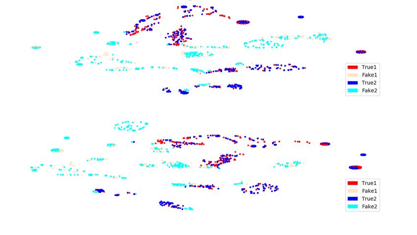
Figure 4: The visualization of true/fake PDs in dark/bright color for IMDB-B. Top: TSNE with kernel distance
induced from Sliced Wasserstein kernel. Bottom: TSNE with bottleneck distance (see appendix).
an intuitive and informal description of the persistent homology induced by a function under a
simple setting. Let f : X → R be a continuous real-valued function defined on a topological
space X. We want to understand the structure of X from the perspective of f . Specifically, let
Xα := {x ∈ X|f (x) < α} denote the sublevel set of X w.r.t. α ∈ R. Now as we sweep X
bottom-up (top down) by increasing the value, the sequence of sublevel (superlevel) sets connected
by natural inclusion maps gives rise to a filtration of X induced by f :
Xα1 ⊂ Xα2 ⊂ ... ⊂ Xαm = X, α1 < α2 < ... < αm (1)
We track how the topological features of sublevel sets change in terms of homology classes. In par-
ticular, as α increases, sometimes new topological features are born at time α, that is, new families
of homology classes are created in Hk (Xα ), the k-th homology group of X. Sometimes, exist-
ing topological features disappear, i.e, some homology classes become trivial in Hk (Xβ ) for some
β > α. The persistent homology captures such birth and death events, and summarizes them in
the so-called persistence diagram Dgk (f ) (We will call it diagram for short when no ambiguity is
raised). Specifically, Dgk (f ) consists of a set of persistence points (α, β) ∈ R2 , where each (α, β)
indicates a k-th homological feature created at α and killed at β. we also call (α, β) persistence
pairing since it pairs two critical values α and β of the filtration function.
In particular, 0 homology is just connected components and can be computed efficiently in
O(α(n)n) using union-find data structure where α(n) is an extremely slow-growing inverse Acker-
mann function.
B.2 E XTENDED P ERSISTENCE H OMOLOGY
Ordinary persistence sometimes may be insufficient to encode the topology of an object X. For
example, when X is a graph, the loops persist forever since they are not filled during the sublevel
filtration. Similarly, upfork branching points (w.r.t. the filtration function f ) are not captured (while
those pointing downwards are detected), since they do not create connected components in the sub-
level filtration.
To address the issues above, extended persistence refines the analysis by also including the super-
level set X α = {x ∈ X : f (x) ≥ α} into the filtration in Eqn (1). Similarly, letting α decrease from
∞ to −∞ gives a sequence of increasing subsets, for which structural changes can be recorded.
In particular, assuming we have a sequence of reals α1 < α2 < · · · < αm such that Xα1 = ∅
11Accepted at the ICLR 2021 Workshop on Geometrical and Topological Representation Learning
(X α1 = X) and Xαm = X (X αm = ∅), we consider the following extended sequence:
∅ =Xα1 ⊆ Xα2 ⊆ · · · ⊆ Xαm = (X; X αm ) (2)
⊆(X; X αm−1 ) ⊆ · · · ⊆ (X; X α2 ) ⊆ (X; X α1 ) = ∅.
where (A; B) denotes a pair of space, and at the homology level, note that the natural map from
Xαm → (X; X αm ) induces an isomorphism. One can then consider the resulting persistent ho-
mology induced by the above extended sequence, and the resulting PDs are called extended PDs.
Persistence pairings in such diagrams have four types, depending on whether the birth and death
happen during the upward filtration (first line in Eqn (2)) or downward filtration (second line in
−
Eqn (2)). In the context of graphs, these types are denoted as Ord0 , Rel1 , Ext+ 0 and Ext1 for
downwards branches, upwards branches, connected components and loops respectively. Overall, we
−
denote Dg(G, f ) = Ord0 (G, f ) ∪ Rel1 (G, f ) ∪ Ext+ 0 (G, f ) ∪ Ext1 (G, f ).
Figure 5: Given the filtration f as height for graph X, the four types of features of graphs and their correspond-
ing persistence points in the extended persistence diagram.
B.3 B OTTLENECK D ISTANCE
Given two PDs D1 and D2 , let Γ : D1 ⊇ A → B ⊆ D2 be a partial bijection between D1 and
D2 . Then for any point x ∈ A, the p-cost of x is defined as cp (x) = kx − Γ(x)kp∞ and for
p
y ∈ (D1 ∪ D2 )\(A ∪ B), the p-cost of y is defined as c0p (y) = ky − π∆ (y)k∞ , where π∆ the
projection onto the diagonal ∆ = {(x, x) : x ∈ R}. The cost of this partial bijection Γ is defined
P P 0 1/p
as cp (Γ) = x c p (x) + c
y p (y) . Finally, define the p-th diagram distance dp as the cost of
the best partial bijection:
dp (D1 , D2 ) = inf cp (Γ), (3)
Γ
where Γ ranges over all partial bijections between D1 and D2 . In the particular case when p = ∞,
the cost of Γ is therefore c(Γ) = max{maxx c1 (x) + maxu c01 (y)}). The corresponding distance
d∞ is often called the bottleneck distance between diagrams D1 and D2 .
B.4 PD S FOR G RAPHS
For graph classification, (Hofer et al., 2017) is the first work introducing a neural network frame-
work to convert PDs into feature vectors for graph classification in an end-to-end data-dependent
way. Perslay (Carriere et al., 2019) unifies many existing featurization such as persistence land-
scape, persistence silhouette (Chazal et al., 2014) and persistence surface as different instances of
a single permutation invariant neural network based on DeepSets (Zaheer et al., 2017). Weighted
Persistence Image Kernel (Zhao & Wang, 2019) (WKPI) is a recently proposed weighted kernel
based on persistence image. WKPI assigns weights for different locations in PDs where weights
are learned from data via gradient descent. Empirically, improved performance over other kernels is
shown for the task of graph classification.
C D IAGRAM S TATISTICS
We list diagram statistics for the shape segmentation task in Table 11. Ave # of PD points (first
row) stands for the average number of persistence points in the diagram for a shape category. A
12Accepted at the ICLR 2021 Workshop on Geometrical and Topological Representation Learning
persistence point is considered as near diagonal if its lifetime is less than one-tenth of the lifetime of
the furthest point in the same diagram.
As we can see in Table 11, most persistence points for mech, bust, cup, bearing, glasses, fish, vase,
teddy are concentrated near diagonal. Those are exactly the same categories on which permuting
diagram yields much better results than not permuting diagrams when PI is used.
Table 11: The diagram statistics for different shape categories in Princeton Shape Benchmark.
Categroy Mech Bust Cup Bearing Glasses Fish Vase Teddy Bird Plier Airplane Table Human Armadillo Chair Hand Fourleg Octopus Ant
Ave # of PD points 11 22.8 15.9 16.9 7.5 15.1 15.7 18.3 18 6.6 12.5 16.6 58.2 78.6 18.8 19.7 31.4 14.6 15.9
# of points near diagonal 9.9 21.5 14.4 15.3 5.6 13.2 13.7 15.1 14.3 2.9 8.5 12.3 53.7 74.1 14.1 14.5 25.9 6.7 7.3
Difference 1.1 1.3 1.5 1.6 1.9 1.9 2 3.2 3.6 3.7 4 4.3 4.4 4.6 4.7 5.1 5.4 7.9 8.6
D PD S FOR M ACHINE L EARNING
D.1 V ECTOR M ETHODS FOR PD S
Persistence Landscape (PL) (Bubenik, 2015) is the first proposed vectorization method for PDs
to overcome some undesirable property of the space of PDs , such as lacking a unique Frechet
mean. This construction is mainly intended for statistical computations, enabled by the vector space
structure of Lp . Given a PD D = {(bi , di )}m i=1 , persistence landscape can be thought of as a
sequence of functions λk : R → R̄ where λk (t) = kth largest value of min (t − bi , di − t)+ .
Persistent Image (PI) (Adams et al., 2017) produces a persistence surface ρB from a PD by taking a
weighted sum of Gaussians centered at each point. The vector representation, named by persistence
image, is created by integrating persistence surface over a grid. In particular, they fix a grid in the
plane with n pixels and assign to each the integral of ρB over that region.
There are at least three parameters involved in the construction of persistence image: 1) a non-
negative weighting function 2) the bandwidth of Gaussian kernel (many other functions can be
chosen but in the original paper only Gaussian is considered) and 3) the resolution of the grid put
over the persistence surface. The authors report that in classification experiments they conducted,
the accuracy is insensitive to the choice of resolution and bandwidth.
D.2 K ERNEL M ETHODS FOR PD S
Persistence Weighted Gaussian Kernel (pwg) (Kusano et al., 2016) essentially utilizes the idea
of kernel mean embedding of distribution, where persistence diagram, treated as a special case of
distribution, can be embedded into RKHS. In particular, Let K, ρ > 0 and D1 and D2 be two PDs.
Let Kρ be the Gaussian kernel with parameter ρ > 0. Let Hρ be the RKHS associated to kρ .
Let µ1 = Σx∈D1 arctan(Kpers(x)p kρ (∗, x)) ∈ Hp be the kernel mean embedding of D1 weighted
by the diagonal distances. Let µ2 be defined similarly. Let τ > 0, the persistence weighted gaussian
kernel Kpwg is defined as the gaussian kernel with bandwidth τ on Hp :
kµ1 −µ2 kH
p
Kpwg (D1 , D2 ) = e− 2t2 (4)
Persistence Scale Space Kernel (pss) (Reininghaus et al., 2015) represents persistence diagram as
sum of Dirac’s delta measure. The persistence scale space kernel is defined as the scalar product of
the solution of the heat diffusion equation with the persistence diagram as an initial value.
The closed form
1 X X (− kp−qk2 ) kp−q̄k2
Kpss (D1 , D2 ) = e 8t − e(− 8t ) (5)
8
p∈D1 q∈D2
can be computed exactly in O(|D1 | ∗ |D2 |) time where q̄ = (y, x) is the symmetric of q = (x, y)
along the diagonal. |D1 | and |D2 | denote the cardinality of the multisets D1 and D2
Sliced Wasserstein Kernel (sw) (Carriere et al., 2017) uses Sliced Wasserstein approximation of
the Wasserstein distance to define a new kernel for PDs. Different from previous multiple kernels, it
13Accepted at the ICLR 2021 Workshop on Geometrical and Topological Representation Learning
is provable not only stable but also discriminative (with a bound depending on the number of points
in the PDs) w.r.t. the first diagram distance w1∞ between PDs.
In particular, the kernel has the following closed-form:
−SW (D1 ,D2 )
Ksw (D1 , D2 ) = e 2σ 2 (6)
where SW (D1 , D2 ), is defined as the sliced Wasserstein distance between PDs.
Persistence Fisher Kernel (pf) (Le & Yamada, 2018) differs from slice Wasserstein kernel in the
sense that the Wasserstein geometry is replaced by Fisher information geometry (metric), which
induces a negative definite distance. The form of Persistence fisher kernel is
kP F (D1 , D2 ) = e−tdF IM (D1 ,D2 ) (7)
where t is a positive scalar and dF IM is the Fisher information metric.
Weighted Persistence Image Kernel (WKPI) (Zhao & Wang, 2019) is recently proposed weighted
kernel that is based on persistence image. In particular, WKPI assigns weight for different location
in the diagram where the weight is learned via gradient descent. The form of WKPI is
(P I(s)−P I 0 (s))2
−
kw (P I, P I 0 ) = ΣN
s=1 w(ps )e
2σ 2 (8)
where PI, PI’ are persistence image, s is the location for each pixel in PI, w is the weight function
that will be learned from data. Note that majority of time to compute WKPI is spent on learning
w(ps ) via stochastic gradient descent.
Table 12: Summary of different kernels for PDs. Here n is the number of diagrams. m is the number of persis-
tence points in the diagram of largest size. M1 is the number of random Fourier feature used for approximating
Gaussian kernel. M2 is the number of directions for approximating Sliced Wasserstein kernel.
pss pwg sw pf WKPI
# of Param 1 3 1 2 2
Exact Comp. Time O(m2 n2 ) O(m2 n2 ) O(m2 log(m)n2 ) O(m2 n2 ) -
Approx. Time - O(M1 mn + M1 n2 ) O(M2 mlog(m)n2 ) O(mn2 ) -
E H YPER - PARAMETERS C HOICE
We chose our hyper-parameters by 10-fold cross-validation on training set. We list the specific
search range for all methods below. All experiments are performed on a single
Persistence Landscape: the number of λk (t) are chosen from {3, 4, 5, 6, 7, 8} and each function
λk (t) is discretized into {50, 100, 200, 300} bins.
Persistence Image: we use the same weight function (Gaussian) in the original paper, the resolution
chosen from {20*20, 30*30}, and bandwidth of Gaussian is selected from {0.01, 0.1, 1, 10, 100}.
Persistence Scale Space Kernel: the parameter t is chosen from 13 values: {0.001, 0.005, 0.01, 0.05,
0.1, 0.5, 1, 5, 10, 100, 500, 1000}.
Sliced Wasserstein Kernel: following the original paper (Carriere et al., 2017), we grid search band-
width from the 5 values: {0.01, 0.1, 1, 10, 100} and the number of slices, i.e., M2 is set to be
10.
Persistence Weighted Gaussian Kernel: we try all the combinations of 5 values from {0.01, 0.1, 1,
10, 100} for bandwidth, and 3 values from {0.1, 1, 10} for both K and ρ, leading to 45 different
sets of parameters.
Persistence Fisher Kernel: there are two hyper-parameters t and τ (for smoothing persistence dia-
gram), both of which are selected from {0.01, 0.05, 0.1, 0.5, 1, 5, 10, 50, 100}.
Pervec/Filvec: The length of the vector is chosen from {100, 200, 300}.
14Accepted at the ICLR 2021 Workshop on Geometrical and Topological Representation Learning
Choice of SVM hyper-parameter: For kernel SVM, the only hyper-parameter C is selected from
{0.01, 1, 10, 100, 1000}. For Pervec and Filvec, Gaussian kernel is utilized where the bandwidth is
selected from {0.01, 0.1, 1, 10, 100}.
Graph Classification: We follow the standard protocol in graph classification literature, i.e., 10-fold
cross-validations, using 9 folds for training and the rest for testing, and repeat the experiments 10
times. We report the average classification accuracies.
F DATASETS D ESCRIPTION
The statistics of the benchmark graph datasets used in the paper are reported in Table 6. Due to
space limitation, we only list the dataset statistics here. We provide detailed dataset description in
the data appendix.
Table 13: Statistics of the benchmark graph datasets.
Datasets graph # class # average nodes # average edges # label #
BZR 405 2 35.75 38.36 +
COX2 467 2 41.22 43.45 +
DD 1178 2 284.32 715.66 +
DHFR 467 2 42.43 44.54 +
FRANKSTEIN 4337 2 16.90 17.88 -
IMDB BINARY 1000 2 19.77 96.53 -
IMDB MULTI 1500 3 13.00 65.94 -
NCI1 4110 2 29.87 32.30 +
PROTEINS 1113 2 39.06 72.82 +
PTC 344 2 14.29 14.69 +
REDDIT 5K 4999 5 508.82 594.87 -
F.1 N ON - ATTRIBUTED G RAPH DATASETS
IMDB-BINARY (Yanardag & Vishwanathan, 2015) is a movie collaboration dataset that consists
of the ego-networks of 1,000 actors/actresses who played roles in movies in IMDB. In each graph,
nodes represent actors/actresses, and there is an edge between them if they appear in the same movie.
These graphs are derived from the Action and Romance genres.
IMDB-MULTI is generated in a similar way to IMDB-BINARY. The difference is that it is derived
from three genres: Comedy, Romance, and Sci-Fi.
REDDIT-BINARY consists of graphs corresponding to online discussions on Reddit. In each graph,
nodes represent users, and there is an edge between them if at least one of them responds to the
other’s comment. There are four popular subreddits, namely, IAmA, AskReddit, TrollXChromo-
somes, and atheism. IAmA and AskReddit are two question/answer based subreddits, and TrollX-
Chromosomes and atheism are two discussion-based subreddits. A graph is labeled according to
whether it belongs to a question/answer-based community or a discussion-based community.
REDDIT-MULTI (5K) is generated in a similar way to REDDIT-BINARY. The difference is that
there are five subreddits involved, namely, worldnews, videos, AdviceAnimals, aww, and mildlyin-
teresting. Graphs are labeled with their corresponding subreddits.
F.2 ATTRIBUTED G RAPHS
PTC (Helma et al., 2001) consists of graph representations of chemical molecules. In each graph,
nodes represent atoms, and edges represent chemical bonds. Graphs are labeled according to car-
cinogenicity on rodents, divided into male mice (MM), male rats (MR), female mice (FM), and
female rats (FR).
PROTEINS (Borgwardt et al., 2005) consist of graph representations of proteins. Nodes represent
secondary structure elements (SSE), and there is an edge if they are neighbors along the amino
acid sequence or one of three nearest neighbors in space. The discrete attributes are SSE types.
The continuous attributes are the 3D length of the SSE. Graphs are labeled according to which EC
top-level class they belong to.
15Accepted at the ICLR 2021 Workshop on Geometrical and Topological Representation Learning
DD (Dobson & Doig, 2003) consists of graph representations of 1,178 proteins. In each graph,
nodes represent amino acids, and there is an edge if they are less than six Angstroms apart. Graphs
are labeled according to whether they are enzymes or not.
NCI1 (Shervashidze et al., 2011; Kriege & Mutzel, 2012) consists of graph representations of 4,110
chemical compounds screened for activity against non-small cell lung cancer and ovarian cancer cell
lines, respectively.
FRANK (Kazius et al., 2005) is a chemical molecule dataset that consists of 2,401 mutagens and
1,936 nonmutagens. Originally, nodes are associated with chemical atom symbols.
BZR, COX2, and DHFR (Sutherland et al., 2003) all are chemical compound datasets. Still, in
each graph, nodes represent atoms, and edges represent chemical bonds. The discrete attributes
correspond to atom types. The continuous attributes are 3D coordinates.
16You can also read