Comparative Analysis of Rain Gauge and Radar Precipitation Estimates towards Rainfall-Runoff Modelling in a Peri-Urban Basin in Attica, Greece - MDPI
←
→
Page content transcription
If your browser does not render page correctly, please read the page content below
hydrology
Article
Comparative Analysis of Rain Gauge and Radar Precipitation
Estimates towards Rainfall-Runoff Modelling in a Peri-Urban
Basin in Attica, Greece
Apollon Bournas *              and Evangelos Baltas

                                          Department of Water Resources and Environmental Engineering, School of Civil Engineering,
                                          National Technical University of Athens, 5 Iroon Polytechniou, 157 80 Athens, Greece; baltas@chi.civil.ntua.gr
                                          * Correspondence: abournas@chi.civil.ntua.gr

                                          Abstract: In this research work, an analysis is conducted concerning the impact on rainfall-runoff
                                          simulations of utilizing rain gauge precipitation measurements against weather radar quantitative
                                          precipitation estimates. The study area is the Sarantapotamos river basin, a peri-urban basin located
                                          in the greater area of Athens, and measurements from a newly installed X-Band weather radar system,
                                          referred to as rainscanner, along with ground rain gauge stations were used. Rainscanner, in contrast
                                          to rain gauges, is able to provide with higher resolution surface precipitation datasets, but due to
                                          signal errors, uncertainty is involved, and thus proper calibration and evaluation of these estimates
                                          must be first performed. In this context, this research work evaluates the impact of adopting different
                                          precipitation datasets and interpolation methods for generating runoff, through the use of a lumped
                                          based rainfall-runoff model. Initially, the analysis focuses on the correlation between the rain gauge
                                          and the rainscanner estimations for each station, as well as for the calculated mean areal precipitation.
                                          The results of the rainfall-runoff simulations show that even though a different spatial and temporal
                                          variability of the rainfall field is calculated through the two datasets, in a lumped-based scheme, the

                                   most important factor that dictates the runoff generation is the amount of total precipitation.
Citation: Bournas, A.; Baltas, E.
Comparative Analysis of Rain Gauge        Keywords: rain gauge; weather radar; rainscanner; mean areal precipitation; Sarantapotamos
and Radar Precipitation Estimates
towards Rainfall-Runoff Modelling in
a Peri-Urban Basin in Attica, Greece.
Hydrology 2021, 8, 29. https://           1. Introduction
doi.org/10.3390/hydrology8010029                Rainfall-runoff modelling depends mainly on the precipitation measurements. The
                                          most used and traditional system of recording precipitation are rain gauge stations. Rain
Received: 31 December 2020
                                          gauge stations provide with point measurement of precipitation and therefore a suitable
Accepted: 7 February 2021
                                          network of such stations is usually implemented over a large area. In hydrology, the study
Published: 10 February 2021
                                          is usually performed on a specified basin scale, therefore a network of such rain gauge
                                          stations that are properly distributed throughout is essential in order to accurately describe
Publisher’s Note: MDPI stays neutral
                                          the spatial variability of a rainfall event. General guidelines by the World Meteorological
with regard to jurisdictional claims in
                                          Organization for implementing such networks are provided, however this is not usually
published maps and institutional affil-
                                          the case, since due to installation costs and orography, the distribution of rain gauges,
iations.
                                          especially on high elevations, is lacking. Moreover, the current demand on quick data
                                          has raised the maintenance costs of ground stations, which require constant powering,
                                          connection to internet and security. For these reasons, more efficient ways, involving
                                          telemetric measurements of precipitation, such as weather radars and satellites, have
Copyright: © 2021 by the authors.
                                          gained increased attention [1]. Weather radars have long been implemented and are
Licensee MDPI, Basel, Switzerland.
                                          considered among the best precipitation data source for modelling [2], while satellite
This article is an open access article
                                          data were only recently implemented and are gaining ground [3]. These systems feature
distributed under the terms and
                                          imminent high spatial and temporal quantitative precipitation estimates (QPE). These
conditions of the Creative Commons
Attribution (CC BY) license (https://
                                          benefits, however, come at a price, since they are subject to quantitate errors [4]. There
creativecommons.org/licenses/by/
                                          is a large number of factors that affect the quality of the QPE, such as systematic errors
4.0/).
                                          due to improper calibration of the rainscanner system, signal attenuation issues and the

Hydrology 2021, 8, 29. https://doi.org/10.3390/hydrology8010029                                             https://www.mdpi.com/journal/hydrology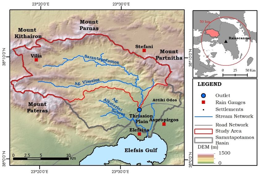
Hydrology 2021, 8, 29                                                                                            2 of 13

                        use of a proper radar reflectivity, Z, to rainfall intensity, R relationship, also known as Z–R
                        relationship, among others [5]. The Z–R relationship is among the most crucial parameters
                        to be configured since it transforms the measured reflectivity fields, Z (mm6 /m3 ), to rainfall
                        intensity, R (mm/h). The relationship is a power law relation in the form of, Z = aRb , where
                        a and b parameters vary depending on the rain droplets’ size distribution of an event [6].
                        Therefore, the Z–R relationship is a static relationship but varies in time and space. The
                        most common approaches are to calibrate the Z–R relationship for use on a specific weather
                        radar based on measurements of a distrometer [7–9], an equipment for measuring the drop
                        size distribution, or the correlation of the QPE with rain gauge measurements [3,10–12].
                        Nevertheless, the parameters of the Z–R relationship should be evaluated for use with only
                        specific storm characteristics, being for instance either convective or stratiform. Only few
                        studies deal with the variability of the Z–R relationship in time space [13,14], while the
                        majority of studies tend to use a one-at-a-time derived Z–R relationship and then apply
                        bias corrections in real time.
                              Regarding rainfall-runoff modelling, the use of radar datasets tends to increase the
                        quality of runoff modelling [15,16], however the raw QPE provided by these systems
                        should be first adjusted based on the rain gauge measurements, since it tends to lead to
                        better accuracy, compared to raw unadjusted radar estimates [17,18]. Gridded datasets
                        tend to perform well with fully distributed models, but semi-distributed and lumped
                        models can be implemented by calculating the Mean Areal Precipitation (MAP) over a
                        basin. One important factor in all studies is the spatial and temporal scale of the analysis.
                        While the spatial scale can be easily configured through modelling, the temporal aspect
                        must not be ignored since weather radar measurements tend to have better correlation
                        with rain gauge measurements when the analysis is performed on coarser scales [2,19,20].
                        Therefore, it is important to notice that the use of higher spatial and temporal resolution
                        datasets does not always translate into more accurate estimations [21,22].
                              In this study, a validation of a newly installed X-Band weather radar, also referred
                        to as rainscanner, is evaluated through performing a comparative analysis between rain
                        gauge measurements and the rainscanner estimates for a peri-urban basin, in the greater
                        region of Athens, in Greece. The rainscanner is located in the facilities of the National
                        Technical University of Athens (NTUA) near the center of Athens, Greece, and features
                        high spatial and temporal scales, with up to 100 × 100 m2 spatial resolution in two min
                        time intervals [23]. This analysis focuses on the generated uncertainty by estimating the
                        rainfall field through different interpolating methods and temporal scales and assessing
                        their impact on the generated hydrographs through rainfall-runoff modelling.

                        2. Materials and Methods
                        2.1. Study Area
                             The study area is the rural part of the Sarantapotamos basin, located in the west part of
                        the Attica region, in Greece, as shown in Figure 1. The Sarantapotamos basin is surrounded
                        by mount Kithairon in the northwest, mount Pastras on the north, mount Parnitha in the
                        northeast and mount Pateras in the west. The main stream is the Sarantapotamos river,
                        which flows throw the valley of Inoi and the Thriasion plain, up to the sea, the Gulf of
                        Elefsis. Other notable sub-streams are Ag. Vlassios, as well as the Soures and Ag. Aikaterini
                        streams that flow within the Mandra settlement and only meet up with Sarantapotamos at
                        Elefsina, just before the sea.
                             The basin is a peri-urban basin case, where the north and largest part of the basin has
                        rural characteristics, while at the south part of the basin, below the Attiki Odos Motorway
                        and the Mandra settlement, extensive urban development is observed. The result of this
                        urbanization has led to the occurrence of numerous flood events, with the most recent
                        and catastrophic being the event of the 14 November 2017, where an intense flash flood
                        event resulted in a total of 24 casualties and huge economic damages within and near
                        the settlement of Mandra [24–26]. Since then, storm water management systems have
                        been designed and implemented for the settlement of Mandra. For this cause, the study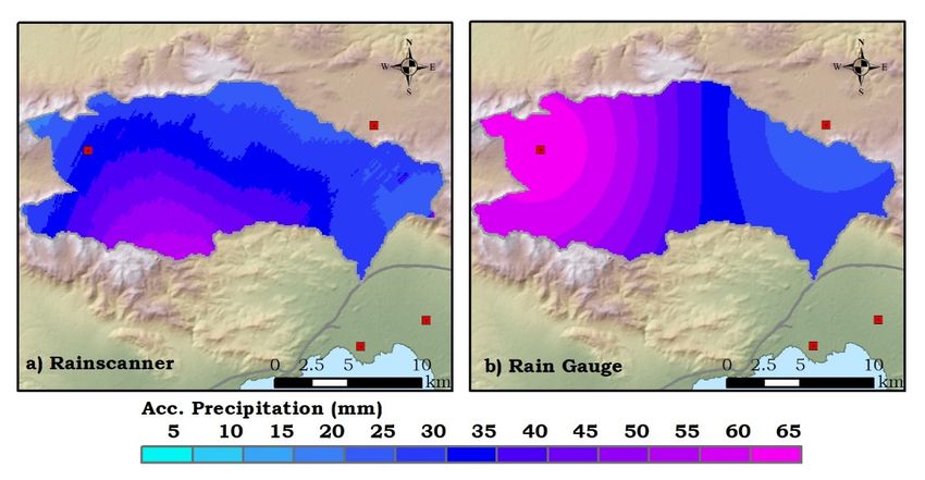
Hydrology 2021, 8, x FOR PEER REVIEW 3 of 12
Hydrology 2021, 8, 29 3 of 13
resulted in a total of 24 casualties and huge economic damages within and near the settle‐
ment of Mandra [24–26]. Since then, storm water management systems have been de‐
signed and implemented for the settlement of Mandra. For this cause, the study area is set
in theisrural
area set inpart of thepart
the rural basin, which
of the is defined
basin, which isby the cross‐section
defined between the
by the cross-section Saranta‐
between the
potamos stream and the and
Attiki 2, with 2
Sarantapotamos stream theOdos
Attikimotorway, covering
Odos motorway, a total area
covering of area
a total 231 km
of 231 km a,
maximum and mean
with a maximum andelevation of 1270ofand
mean elevation 470
1270 andm,470
respectively. WithinWithin
m, respectively. this part,
this the most
part, the
notable settlements
most notable are Vilia,
settlements are Oinoi, Pournari
Vilia, Oinoi, and Lefka,
Pournari locatedlocated
and Lefka, near the banks
near the of Saran‐
banks of
tapotamos,
Sarantapotamos,and Ag.andGeorgios and Paleochori
Ag. Georgios located
and Paleochori near the
located nearbanks of Ag.
the banks ofVlassios. The
Ag. Vlassios.
study area is
The study theislargest
area rural rural
the largest basinbasin
withinwithin
the region of Attiki,
the region wherewhere
of Attiki, data from
datathe
fromnewly
the
newly installed
installed rainscanner
rainscanner are available.
are available.
Figure 1.
Figure The Sarantapotamos
1. The Sarantapotamos basin,
basin, the
the study
study area
area and the rain gauge network.
The land
The land cover
cover of
of the
the region
regionisismostly
mostlyforest-based,
forest‐based,with
withagricultural
agricultural activity found
activity in
found
the plains of Oinoi and Lefka. Sarantapotamos stream has a total length of
in the plains of Oinoi and Lefka. Sarantapotamos stream has a total length of 38 km, where38 km, where
28 km
28 km lies
lies within
within the
the study
study area.
area. The
The first
first 20
20 km
km have
have aa west
west toto east
east direction, only to
direction, only to
switch to a southern direction for the remainder. This direction tends to have
switch to a southern direction for the remainder. This direction tends to have an impact an impact on
thethe
on generation
generationof high runoff
of high peaks,
runoff sincesince
peaks, in most cases,cases,
in most the storm movement
the storm in the region
movement in the
also has the same direction, and thus the accumulation of runoff is accelerated.
region also has the same direction, and thus the accumulation of runoff is accelerated.
2.2. Data Used
2.2. Data Used
For this study, a rainfall event that occurred in November 2019 from 21:40 UTC+2 of the
For this study, a rainfall event that occurred in November 2019 from 21:40 UTC+2 of
24th up until 06:00 UTC+2 of the 25th, was studied. The event resulted in a low barometric
the 24th up until 06:00 UTC+2 of the 25th, was studied. The event resulted in a low baro‐
pressure that was created on 24 November 2019, over Italy, and a cold front extending
metric
almostpressure
throughout thatsouthwestern
was created on 24 November
Greece. 2019, over
The barometric Italy,
system wasand a cold frontasex‐
strengthened it
tending almost throughout southwestern Greece. The barometric
moved to the east over the Ionian Sea and continued to deepen for the next system was six
strength‐
hours
ened as it moved
and moved quicklyto to
thethe
east over
east, the Ionian
affecting Sea Greece
central and continued to deepen
and Attica. The systemfor the next six
produced
hours
high-intensity rainfall events, with large sums of cumulative rain with strong winds.pro‐
and moved quickly to the east, affecting central Greece and Attica. The system By
duced
applying high‐intensity
well-known and rainfall
usedevents, with
Intensity large sums
Duration of cumulative
Frequency (IDF) curves rain with for
derived strong
the
winds.
MandraBy applying
station [27],well‐known
the studied and
eventused
hadIntensity Duration
a 5- to 10-year Frequency
return period. (IDF) curves de‐
rivedTwo
for the
sets of rainfall measurements were used in this study. Thereturn
Mandra station [27], the studied event had a 5‐ to 10‐year period.
first are ground
Two sets of rainfall measurements were used in this study. The first
rain gauge stations, as well as gridded precipitation datasets acquired from the NTUA are ground rain
gauge stations, as well as gridded precipitation datasets acquired from
rainscanner system. The rain gauge stations used in this study are part of the National the NTUA rain‐
Observatory of Athens Automatic Network (NOAAN), which provides with high-quality
10 min precipitation height datasets with good coverage of the entire Hellenic continent [28].
The network is constantly updating with the addition of new stations, but for the studied
event, only one station, the Vilia station, is located within the study area. Three more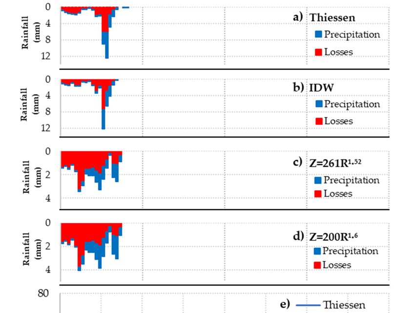
Hydrology 2021, 8, 29 4 of 13
stations, the Stefani, the Aspropirgos and the Elefsina stations, in close proximity to
the basin, were therefore used, in order to properly calculate the MAP within the basin.
As seen in Figure 1, the rain gauge distribution within the basin is not optimal, since
only the Vilia station is located in high elevation, whereas Aspropirgos and Elefsina are
located further away, near the coast. The Stefani station is located near the basin, and will
therefore contribute substantially to the MAP, but is located on the other side of mount
Partnitha, which will most likely have a negative effect of MAP estimations, since due
to orography and storm movement, the west part will record higher precipitation values
than the east. By applying the Thiessen polygons interpolation method, the corresponding
station weights were calculated as 54%, 43%, 2% and 1% for stations Vilia, Stefani, Elefsina
and Aspropirgos, respectively.
On the other hand, the NTUA rainscanner estimates are based on measurements of
reflectivity in a gridded format of a 100 m × 100 m pixel size and 2 min temporal scale.
Proper ground clutter corrections were applied, and the datasets were aggregated into
10 min intervals to match the rain gauges scale. In order to utilize the datasets, a suitable
Z–R relationship must first be used in order to transform the reflectivity values (Z) into
rain rate (R) based on the expression, Z = aRb , where the values of parameters a and b
depend upon the droplets’ size distribution of the specific event. Since such measurements
were not available, two set of parameters were used based on previous studies. First,
the well-known Marshal n’ Palmer equation, Z = 200R1.6 , was used [6], which is suitable
for general use, as well as the equation Z = 261R1.52 , which was derived by analyzing
distrometer measurements of rainfall events within the area of Athens [7].
2.3. Rainfall-Runoff Model
As is the case in the majority of subbasins in the region, the study area is an ungauged
basin, and no discharge datasets were available. For estimating the generated runoff,
the synthetic Soil Conservation Service (SCS) dimensionless United Hydrograph (UH)
was used, which due to its simplicity and low data requirements, has been used with
success in various studies in Greece [29]. The model has one parameter, the basin lag,
i.e., the time difference between the center of mass of rainfall excess and the peak of
the UH. The parameter can be evaluated as a fraction of the time of concentration, with
0.6 as the suggested value, plus half the time interval step. The time of concentration
can be calculated through the empirical relationships, such as the Giandotti equation,
which is reported to have better results in Mediterranean basins than other empirical
methods [30,31]. The concentration time was calculated, equal to 6.70 h.
Precipitation losses were calculated through the use of the Soil Conservation Service-
Curve Number (SCS-CN) method [32]. The SCS-CN method is a widely used and efficient
method for estimating precipitation losses in ungauged basins since it only requires two pa-
rameters, i.e., the CN that specifies the soil storage capacity, S, and the initial abstraction,
which is expressed as a percentage of S, with 0.2 as the suggested value [30]. The derivation
of CN was performed using Geographical Information Systems (GIS) tools, by combining
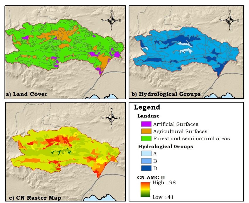
the Corine Land Cover (CLC) of 2018, geological maps and respected CN tables [33]. In
Figure 2, the above raster maps are presented. For the CLC map, although shown for
classification level one, the analysis was performed on CLC level two. Since a lumped
approach was taken for the simulations, the mean value of the CN raster was calculated as
the sole CN for the entire basin. In order to evaluate the hydrological condition of soils
before the event, the seven days antecedent precipitation index (API) and the normalized
antecedent precipitation index (NAPI) [34] were calculated for each station. The API value
for stations Vilia, Elefsina, Asporirgos and Stefani was 31.96, 21.80, 20.60 and 28.47 mm,
while the NAPI was calculated at 2.94, 2.3, 2.30 and 1.77 mm, respectively. Considering
the location of each station, i.e., the high coverage of the study area by stations Vilia and
Stefani, averaging at 97% through the Thiessen polygon method, the values indicate that
wet antecedent conditions were present prior to the event, and thus the Antecedent Mois-
ture Conditions (AMC), AMC-III was calculated through AMC-II. The mean CN used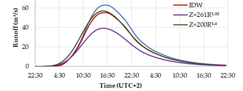
and 28.47 mm, while the NAPI was calculated at 2.94, 2.3, 2.30 and 1.77 mm, respectively.
Considering the location of each station, i.e., the high coverage of the study area by sta‐
Hydrology 2021, 8, 29 tions Vilia and Stefani, averaging at 97% through the Thiessen polygon method, the values5 of 13
indicate that wet antecedent conditions were present prior to the event, and thus the An‐
tecedent Moisture Conditions (AMC), AMC‐III was calculated through AMC‐II. The mean
CN used in the simulations was 83. Finally, regarding baseflow, as in the case of most
in the simulations was 83. Finally, regarding baseflow, as in the case of most streams in
streams in the Attica region, Sarantapotamos does not feature any form of baseflow. All
the Attica region, Sarantapotamos does not feature any form of baseflow. All simulations
simulations were performed using the Hydrologic Engineering Center‐Hydrologic Mod‐
were performed using the Hydrologic Engineering Center-Hydrologic Modelling System
elling System (HEC‐HMS) model. HEC‐HMS is a rainfall‐runoff modelling platform de‐
(HEC-HMS) model. HEC-HMS is a rainfall-runoff modelling platform developed by the
veloped by the United States (US) Army Corps of Engineers [35], which integrates the use
United States (US) Army Corps of Engineers [35], which integrates the use of sub-models,
of sub‐models, in order to model different aspects of the rainfall‐runoff process, and has
in order to model different aspects of the rainfall-runoff process, and has been applied with
been applied with success in various studies in Greece [36–38].
success in various studies in Greece [36–38].
Figure
Figure2.2.Geomorphological
Geomorphologicalanalysis—Curve
analysis—Curve Number (CN) (CN) map
map derivation
derivationprocess,
process,(a)
(a)Corine
CorineLand
Land Cover
Cover (CLC),(CLC), classification
classification level level one,hydrological
one, (b) (b) hydrological groups,
groups, (c)raster
(c) CN CN raster
map. map.
2.4.Mean
2.4. MeanAreal
ArealPrecipitation
PrecipitationCalculation
CalculationMethods
Methods
Whenadopting
When adoptingaalumped
lumpedbasin
basinrainfall‐runoff
rainfall-runoffscheme,
scheme,the therain
raingauge
gaugeprecipitation
precipitation
datasets must be first converted into MAP. Regarding rain gauges, as
datasets must be first converted into MAP. Regarding rain gauges, as point measure‐point measurements,
there are
ments, several
there are methods by whichby
several methods thiswhich
can bethis
achieved.
can beThe most common
achieved. The most method
commonis by
applying
method weights
is by intoweights
applying each station’s measurements
into each and calculating
station’s measurements the MAP asthe
and calculating theMAP
sum
as the sum of the weighted precipitation. The easiest way to calculate these weightsthe
of the weighted precipitation. The easiest way to calculate these weights is through is
calculation
through the of the Thiessen
calculation polygons,
of the Thiessenwhich dictate
polygons, the area
which of influence
dictate the area of of influence
each stationof
within
each a specified
station within basin. The percentage
a specified of the area of
basin. The percentage to the
the total
area toarea
theoftotal
the basin
area ofisthe
the
actual weight used for MAP calculation. The method dictates that every
basin is the actual weight used for MAP calculation. The method dictates that every pointpoint within the
area of a designated stations’ Thiessen polygon would have the same precipitation
within the area of a designated stations’ Thiessen polygon would have the same precipi‐ value
as that of the station. While the method is rather simple, when good distribution of the
tation value as that of the station. While the method is rather simple, when good distribu‐
station’s location within the basin is present, the method performs well.
tion of the station’s location within the basin is present, the method performs well.
In cases where bad distribution or a limited number of stations are present, the results
may not be representative. Therefore, other interpolation methods can be utilized, such as
the inverse distance weighting (IDW) or more complex methods such as ordinary Kriging.
In IDW, a gridded precipitation dataset is constructed, utilizing weights based upon the
inverse squared distance of each cell for all stations. Following the creation of this dataset,
the MAP is easily calculated as the mean value of the raster dataset for each time interval.may not be representative. Therefore, other interpolation methods can be utilized, such as
the inverse distance weighting (IDW) or more complex methods such as ordinary Kriging.
In IDW, a gridded precipitation dataset is constructed, utilizing weights based upon the
inverse squared distance of each cell for all stations. Following the creation of this dataset,
Hydrology 2021, 8, 29 the MAP is easily calculated as the mean value of the raster dataset for each time interval.
6 of 13
Finally, regarding the rainscanner measurements, being gridded datasets, the MAP is cal‐
culated as in the case of IDW.
Finally,
3. Results andregarding the rainscanner measurements, being gridded datasets, the MAP is
Discussion
calculated as in the case of IDW.
3.1. Precipitation Analysis
3. Results
First and Discussion
a correlation analysis is performed between each individual station’s timeseries
3.1. Precipitation Analysis
and the timeseries derived from the rainscanner. The 10 min datasets were aggregated
into 30 minFirst a correlation
and analysis
1 h intervals, is performed
in order to assessbetween each individual
the temporal influence. station’s timeseries
In Figure 3, the
and
scatter the are
plots timeseries
shown,derived
for timefrom the rainscanner.
intervals of 30 min andThe110 h, min
whiledatasets
in Table were aggregated
1, the correla‐
into 30 minvalues
tion coefficient and 1forh intervals,
each timein order to
interval areassess the temporal
presented. influence.
It is obvious that byInassessing
Figure 3,
the scatter plots are shown, for time intervals of 30 min and 1 h,
the datasets in high temporal scale, such as 10 min, low correlation is observed, butwhile in Table 1, the
by
correlation coefficient values for each time interval are presented. It is obvious
aggregating, up to 1 h, the correlation is getting stronger. In the stations’ scale, the corre‐ that by
assessing the datasets in high temporal scale, such as 10 min, low correlation is observed,
lations on the 10 min datasets are lower than 0.10, while on the 30 min datasets, they are
but by aggregating, up to 1 h, the correlation is getting stronger. In the stations’ scale, the
between 0.11 and 0.25, and on the 1 h scale, the correlation is approximately 0.40, apart
correlations on the 10 min datasets are lower than 0.10, while on the 30 min datasets, they
from station Vilia which reports low correlation in all cases. As seen in Figure 3, it seems
are between 0.11 and 0.25, and on the 1 h scale, the correlation is approximately 0.40, apart
that an overestimation
from is performed
station Vilia which reports lowby the rainscanner
correlation in allin low As
cases. precipitation
seen in Figurevalues,
3, it while
seems
an underestimation is performed on higher values.
that an overestimation is performed by the rainscanner in low precipitation values, while
an underestimation is performed on higher values.
10 10
Vilia 1:1 Vilia 1:1
Stefani Stefani
Rainscanner (mm / 30 min)
Rainscanner (mm / 1 h)
8 Eleusina 8 Eleusina
Aspropirgos Aspropirgos
6 6
4 4
2 2
0 0
0 2 4 6 8 10 0 2 4 6 8 10
Rain Gauge (mm / 30 min) Rain Gauge (mm / 1 h)
(a) (b)
FigureFigure
3. Rainscanner and rain
3. Rainscanner andgauge scatter
rain gauge plots,
scatter (a) on
plots, (a)aon
30amin temporal
30 min scale,
temporal and
scale, (b)(b)
and onon
a 1a 1h htemporal
temporalscale.
scale.
TableTable
1. Correlation coefficient
1. Correlation for for
coefficient different time
different interval
time scales.
interval scales.
Entire
Entire Event
Event Excluding
Excluding04:00–06:00
04:00–06:00
Station
Station
10 min
10 min 30 min
30 min 1 1hh 1010min
min 30 min
30 min 11hh
Vilia
Vilia 0.04
0.04 0.11
0.11 0.07
0.07 0.67
0.67 0.72
0.72 0.72
0.72
Stefani
Stefani 0.03
0.03 0.11
0.11 0.49
0.49 0.36
0.36 0.67
0.67 0.83
0.83
Eleusina
Eleusina 0.02
0.02 0.25
0.25 0.45
0.45 0.57
0.57 0.66
0.66 0.68
0.68
Aspropirgos 0.07 0.19 0.41 0.54 0.46 0.32
Aspropirgos 0.07 0.19 0.41 0.54 0.46 0.32
Interpolated Timeseries 1
Interpolated Timeseries 1
Thiessen 1 0.22 0.21 0.30 0.57 0.65 0.71
IDW 1 0.19 0.20 0.28 0.45 0.56 0.72
1 Correlation coefficients calculated against the Rainscanner Mean Area Precipitation (MAP) derived by using
relationship Z = 200R1.6 .In Figure 4, the timeseries of the MAP derived from the IDW method f
gauges and the Z = 200R1.6 relationship for the radar measurements are presen
plots along with the precipitation accumulation timeseries in lines. MAP derive
Hydrology 2021, 8, 29 7 of 13
Thiessen method and the Z = 261R1.52 relationship were highly correlated with
results, and therefore they were not plotted for visualization purposes. Whi
sets, the accumulative
In Figure precipitation
4, the timeseries of the MAPisderivedequal from
at 42themm,IDW there
method is afor
difference
the rain in th
variability
gauges and theof Zthe rainfall
= 200R 1.6 field. Infor
relationship thetherainscanner
radar measurementscase, area near linear
presented accumula
in bar
plots along with the precipitation
served, whereas in the case of the accumulation timeseries in lines. MAP derived
rain gauges, less precipitation is recorded from
the Thiessen method and the Z = 261R1.52 relationship were highly correlated with the
hours, only to peak at approximately 04:30 until 06:00. In the same time period
above results, and therefore they were not plotted for visualization purposes. While for
scanner
both sets,measures little to
the accumulative no data, which
precipitation is equal isat evidence
42 mm, there of isabnormal
a differencebehavior.
in the Sin
gauge
temporal measurements’ quality
variability of the rainfall isInnot
field. in question,
the rainscanner case,the most
a near linearstand out cause of
accumulation
is observed, whereas in the case of the rain gauges, less precipitation is recorded in the
would most likely be in radar signal errors, such as signal attenuation or overs
first hours, only to peak at approximately 04:30 until 06:00. In the same time period, the
the actual storm
rainscanner measures cloud.
little toThe study
no data, whicharea is located
is evidence near the
of abnormal limit of
behavior. thethe
Since rainscan
thus with measurements’
rain gauge a preset 2 degrees quality isofnot
thein radar
question, beam angle,
the most standthe
outmeasurements
cause of this error are tak
as 2 km difference altitude compared to those in the ground overshooting
would most likely be in radar signal errors, such as signal attenuation or surface. X‐Band of rad
the actual storm cloud. The study area is located near the limit of the rainscanner range,
have weaker signals, thus in some cases, where a storm cloud is in between th
thus with a preset 2 degrees of the radar beam angle, the measurements are taken as high
ner
as 2and further altitude
km difference targeted locations,
compared heavy
to those in the underestimation
ground surface. X-Band of radar
the rainfall
systems field i
may
have occur. By removing
weaker signals, thus in some thecases,
specific
wheretimea storminterval,
cloud is inthe correlation
between in all statio
the rainscanner
and further targeted locations, heavy underestimation of the rainfall field in that area
MAP increases, above 0.6 in most cases, as seen in Table 2. This indicates that o
may occur. By removing the specific time interval, the correlation in all stations and the
rainscanner
MAP increases,measurements
above 0.6 in most are cases,correlated,
as seen in Table but2. sensitive
This indicates applications
that overall, the on locat
rainscanner ranges should
rainscanner measurements be avoided,
are correlated, or work
but sensitive in conjunction
applications on locations with rain gaug
at the rain-
scanner Regardless,
ments. ranges should be inavoided, or work work,
this research in conjunction with rain were
the datasets gauge used measurements.
“as is”, in ord
Regardless, in this research work, the datasets were used “as is”, in order to validate the
date the current measurements and their impact on the rainfall‐runoff simulat
current measurements and their impact on the rainfall-runoff simulations.
40 50
Accumulative Precipitation (mm)
Rain gauge (IDW)
35
Precipitation Depth (mm)
Radar 40
30
Acc Gauge
25 30
Acc Radar
20
15 20
10
10
5
0 0
22:00 0:00 2:00 4:00 6:00 8:00
Time (UTC +2)
Figure 4. Mean areal precipitation and accumulative precipitation (Acc) for the rain gauge and radar
Figure 4. Mean areal precipitation and accumulative precipitation (Acc) for the rain gau
estimations through the IDW and Z = 200R1.6 precipitation products.
radar estimations through the IDW and Z = 200R1.6 precipitation products.
Regarding the total precipitation recorded by both measurements, 44, 41
mm were calculated for the for the rain gauge Thiessen, IDW methods and the r
Z = 261R1.52 and Z = 200R1.6, respectively. While the Thiessen and IDW metho
show any significant difference, the impact of the Z–R relationship is crucial. Lo
of parameters a and b lead to higher precipitation estimates, while higher valu
usually better suited in convective type storms. Finally, in Figure 5, the spatial dPEER REVIEW 8 of 12
Hydrology 2021, 8, 29 8 of 13
of the total precipitation is shown, for rain gauge MAP through the IDW method and the
rainscanner estimates through relationship Z = 200R1.6. In the rain gauges case, the spatial
Table 2. Main characteristics of the generated hydrographs.
distribution of rainfall is dictated only by the station’s locations and their corresponding
= 261R1.52 Z = 200R1.6
measurements, thus the maximum Characteristic
precipitationThiessen
is foundIDW at Vilia Zstation, located on the
Peak Discharge (m3 /s) 63 55 39 57
northwest part of the Total
basin. In the rainscanner44 case, the 41
Precipitation (mm)
distribution35 is affected 42by the
actual storm cloud movement, thus the maximum
Losses (mm) 29 total 28precipitation 26 occurred28in the
Excess (mm) 15 13 9 14
southwest, and specifically over the mount Pateras.
Runoff Volume (103 m3 ) 3468
This difference
3044
can2211
have an impact 3222
on
rainfall‐runoff simulations
Timewhere a semi‐distributed
to Peak (hours) 18.0 or fully
17.6 distributed17.5 approach17.5 is con‐
sidered, which is not the case of this work. However, the error of applying rain gauge
measurements as the sole Regarding the totalof
datasets precipitation recordedis
precipitation by both measurements,
highlighted. 44, 41, 42 and 39and
Rainscanner mm
were calculated for the for the rain gauge Thiessen, IDW methods and the rainscanner
weather radar measurements in general may involve increased uncertainty, but the added
Z = 261R1.52 and Z = 200R1.6 , respectively. While the Thiessen and IDW methods do not
value of the spatial variability of rainfall
show any significant cannot
difference, be denied.
the impact of the Z–R relationship is crucial. Lower values
of parameters a and b lead to higher precipitation estimates, while higher values of a are
usually of
Table 2. Main characteristics better
thesuited in convective
generated type storms. Finally, in Figure 5, the spatial distribution
hydrographs.
of the total precipitation is shown, for rain gauge MAP through the IDW method and the
rainscanner estimates through relationship Z = 200R1.6 . In the rain1.52
Characteristic Thiessen IDW Z = 261R gauges Z case, the spatial
= 200R1.6
distribution of rainfall is dictated only by the station’s locations and their corresponding
Peak Discharge (m3/s) thus the maximum
measurements, 63 precipitation
55 is found at39Vilia station, located57 on the
northwest
Total Precipitation (mm) part of the basin. In44the rainscanner
41 case, the distribution
35 is affected
42 by the
actual storm cloud movement, thus the maximum total precipitation occurred in the
Losses (mm)
southwest, and specifically over 29 the mount 28 26
Pateras. This difference can have 28an impact
Excess (mm)
on rainfall-runoff simulations15 13
where a semi-distributed 9 distributed approach
or fully 14 is
considered, which is not the case of this work. However, the error of applying rain gauge
Runoff Volume (103 m3) 3468 3044 2211 3222
measurements as the sole datasets of precipitation is highlighted. Rainscanner and weather
Time to Peakradar
(hours)
measurements in general 18.0
may involve17.6 17.5 but the added
increased uncertainty, 17.5value of
the spatial variability of rainfall cannot be denied.
Figure 5. Accumulative precipitation, (a) rainscanner estimates through Z = 200R1.6 , (b) rain gauges through IDW.
Figure 5. Accumulative precipitation, (a) rainscanner estimates through Z = 200R1.6, (b) rain gauges
through IDW.
3.2. Rainfall‐Runoff Simulations
In Figure 6, the simulated hydrographs for all precipitation estimates are presented,
along with their respective rainfall timeseries. Specifically, the simulations were per‐
formed for four datasets of precipitation, two based on rain gauge measurements, i.e.,Hydrology 2021, 8, 29 9 of 13
3.2. Rainfall-Runoff Simulations
In Figure 6, the simulated hydrographs for all precipitation estimates are presented,
along with their respective rainfall timeseries. Specifically, the simulations were performed
for four datasets of precipitation, two based on rain gauge measurements, i.e., MAP derived
by Thiessen polygons and IDW methods, and two based on rainscanner estimations, i.e.,
by applying two different Z–R relationships, Z = 200R1.6 and Z = 261R1.52 . The simulations
were performed in 30 min time steps. In Table 2, the main characteristics of the flood
hydrographs are presented. In Figure 6, the individual hydrographs for each dataset are
Hydrology 2021, 8, x FOR PEER REVIEW shown, along with their corresponding precipitation and losses. The difference in the 9
temporal variability of rainfall is obvious between the rain gauge simulations, Figure 6a,b,
and those from derived from the rainscanner, Figure 6c,d.
Figure 6. Rainfall-runoff simulations for each dataset. Rainfall timeseries for each dataset are shown
Figure 6. Rainfall‐runoff simulations for each dataset. Rainfall timeseries for each dataset are
in, (a) Thiessen; (b) IDW; (c) Z = 200R1.6 ; (d) Z = 261R1.52 ; (e) simulated hydrographs.
shown in, (a) Thiessen; (b) IDW; (c) Z = 200R1.6; (d) Z = 261R1.52; (e) simulated hydrographs.
A small deviation is observed in all hydrographs. Overall, all precipitation dat
showed equal hydrographs, except in the case of the first Z–R relationship, where the
discharge and runoff volume is lower than in the other cases. Concerning the two M
products derived from the rain gauge measurements, the difference between the Thie
and the IDW methods was 7.70 m3/s on the peak discharge, which resulted in an oHydrology 2021, 8, 29 10 of 13
A small deviation is observed in all hydrographs. Overall, all precipitation datasets
showed equal hydrographs, except in the case of the first Z–R relationship, where the peak
discharge and runoff volume is lower than in the other cases. Concerning the two MAP
products derived from the rain gauge measurements, the difference between the Thiessen
and the IDW methods was 7.70 m3 /s on the peak discharge, which resulted in an only
3 mm difference on total precipitation, while the time to peak was slightly lower in the
IDW case. The difference in the Z–R relationship results lie in the difference in the amount
of precipitation, since by using the relationship Z = 200R1.6 , more precipitation is estimated.
By using Z = 200R1.6 , the total precipitation was calculated at 7 mm, i.e., 20%, more than
the precipitation estimated by using Z = 261R1.52 , which resulted in 17.90 m3 /s, i.e., 46%,
more peak discharge and runoff volume generation.
Finally, comparing the rain gauge measurements with the rainscanner, it seems that the
best correlation is seen when utilizing IDW for MAP based on the rain gauge measurements,
with the Z = 200R1.6 relationship. The difference between these two sets was less than
3% on the generated peak discharge and runoff volume. It is found that when a lumped
scheme is used, the most important factor for achieving the best correlation between the
two datasets is the total amount of precipitation, regardless of the temporal and spatial
correlation of the precipitation timeseries. Regarding the temporal distribution of rainfall, it
is estimated that any difference found between the datasets is actually diminished through
the calculation of precipitation losses, even in the case of wet AMC-III conditions, where
the least number of losses was calculated. Nevertheless, it is important to notice that
the effect of the Z–R relationship upon the generated hydrograph is rather significant,
therefore increased attention should be made when applying a specific Z–R relationship. It
is suggested that the combined use of rainscanner and rain gauge measurements should
be used, in order to obtain the best spatial detail of the rainfall field from the rainscanner
measurements and the quality of the rain gauge station datasets.
4. Conclusions
In this study the impact of adopting different mean areal precipitation calculations and
their impact on generated hydrographs was performed. The comparisons were performed
on a peri-urban basin, the Sarantapotamos river basin, known for its recent catastrophic
flood events. The analysis was performed on two areas, first involving a correlation analysis
between the different precipitation products, derived from the rain gauge and rainscanner
measurements, and secondly regarding their impact on the generated hydrograph through
rainfall-runoff modelling.
It was shown that the correlation between the rainscanner and rain gauge datasets
is affected by the temporal scale of the analysis, where at fine scales of 10 min, the corre-
lation is not good, whereas at larger scales of 30 min to 1 h, the datasets showed better
correlation. However, on average, the rainscanner measurements tended to overestimate
low precipitation values, and underestimate high values. It is therefore suggested that
weather radar bias corrections should only be applied on the time scale of the proposed
analysis. Concerning the estimated total MAP for the studied event, it was found that
higher values are estimated through the use of the Thiessen polygons method, in contrast
with IDW, although the difference was a few mm of precipitation. However, the Thiessen
method failed to recreate the spatial variability of the rainfall field, and as such, the IDW is
considered a better estimate. Regarding the rainscanner measurements, it was shown that
by using a different Z–R relationship, even with small changes in the parameter values, a
significant difference of up to 20 mm was found on the total MAP, which highlights the
impact of the used Z–R relationship. The best correlation between the two datasets was
found when using the IDW method for the rain gauges and the Z = 200R1.6 relationship.
In this case, although the total MAP was equally estimated, the spatial variability of the
rainfall field was different in each case, since in the IDW method, it is dictated by the
station’s location and measurements, whereas in the rainscanner, it concerns actual rainfall.Hydrology 2021, 8, 29 11 of 13
In the studied event, the IDW method calculated the maximum rainfall in the northwest
part of the basin, whereas in the rainscanner, the maximum was located in the southwest.
Finally, regarding the impact on rainfall-runoff simulations, it was found that when a
lumped scheme was used, the main parameter that led to equal runoff volume generation
was the total precipitation, regardless of its temporal and spatial variability between the
two datasets. While a certain amount of temporal correlation between the two datasets
is always met, since they are measuring the same rainfall volume, the impact of it is
diminished through the calculation of precipitation losses. Results showed that for the
studied event, the best correlation between the two datasets was met when adopting the
IDW and the Z = 200R1.6 , since they feature the same total precipitation values. Finally, the
difference between the two Z–R relationships should also be mentioned, since, as stated, a
small change in the values of parameters a and b can lead to up to a 20% difference in the
estimated total precipitation, which led to a 46% difference on the calculated peak discharge.
The usage of an inappropriate Z–R relationship can lead to wrong rainfall estimates, which
in turn multiply the extent of the errors generated in the runoff calculations.
Future research will focus on evaluating the spatial variability of the rainfall fields
on the generated hydrograph through implementation of semi-distributed and fully dis-
tributed rainfall-runoff models for multiple events measured in the region. Observed
runoff, if available, should be utilized to calibrate and validate the used model, in order
to minimize any uncertainty generated by the added parameters. Finally, a rain gauge–
rainscanner error correction scheme could also be evaluated. Through this study, it is also
acknowledged that the overall quality and correlation of the rainscanner estimates with
rain gauge data depend heavily on the spatial and temporal scale of the analysis, thus the
investigation of Z–R relationship calibration and bias corrections in such small scales could
be considered important for highly detailed early warning systems.
Author Contributions: Conceptualization, A.B. and E.B.; methodology, A.B.; software, A.B.; valida-
tion, A.B. and E.B.; formal analysis, A.B.; investigation, A.B.; resources, A.B. and E.B.; data curation,
A.B.; writing—original draft preparation, A.B.; writing—review and editing, A.B. and E.B.; visualiza-
tion, A.B.; supervision, E.B.; project administration, E.B.; funding acquisition, A.B. All authors have
read and agreed to the published version of the manuscript.
Funding: This research is co-financed by Greece and the European Union (European Social Fund-
ESF) through the Operational Programme “Human Resources Development, Education and Lifelong
Learning” in the context of the project “Strengthening Human Resources Research Potential via
Doctorate Research” (MIS-5000432), implemented by the State Scholarships Foundation (IKΥ).
Institutional Review Board Statement: Not applicable.
Informed Consent Statement: Not applicable.
Data Availability Statement: The data presented in this study are available on request from the
corresponding author.
Acknowledgments: Authors would like to thank the Institute of Environmental Research and
Sustainable Development of the National Observatory of Athens for the supply of the rain gauge
precipitation measurements in the study area. This research was conducted in the framework of the
corresponding author’s PhD study funded by the Greek State Scholarships Foundation (IKY).
Conflicts of Interest: The authors declare no conflict of interest.
References
1. Berenguer, M.; Corral, C.; Sánchez-Diezma, R.; Sempere-Torres, D. Hydrological Validation of a Radar-Based Nowcasting
Technique. J. Hydrometeor. 2005, 6, 532–549. [CrossRef]
2. Price, K.; Purucker, S.T.; Kraemer, S.R.; Babendreier, J.E.; Knightes, C.D. Comparison of Radar and Gauge Precipitation Data in
Watershed Models across Varying Spatial and Temporal Scales. Hydrol. Process. 2014, 28, 3505–3520. [CrossRef]
3. Gilewski, P.; Nawalany, M. Inter-Comparison of Rain-Gauge, Radar, and Satellite (IMERG GPM) Precipitation Estimates
Performance for Rainfall-Runoff Modeling in a Mountainous Catchment in Poland. Water 2018, 10, 1665. [CrossRef]Hydrology 2021, 8, 29 12 of 13
4. Villarini, G.; Krajewski, W.F. Review of the Different Sources of Uncertainty in Single Polarization Radar-Based Estimates of
Rainfall. Surv. Geophys. 2010, 31, 107–129. [CrossRef]
5. Pathak, C.; Curtis, D.; Kitzmiller, D.; Vieux, B. Identifying and Resolving the Barriers and Issues in Using Radar-Derived Rainfall
Estimating Technology. J. Hydrol. Eng. 2013, 18, 1193–1199. [CrossRef]
6. Marshall, J.S.; Palmer, W.M.K. The Distribution of Raindrops with Size. J. Meteorol. 1948, 5, 165–166. [CrossRef]
7. Baltas, E.A.; Panagos, D.S.; Mimikou, M.A. An Approach for the Estimation of Hydrometeorological Variables Towards the
Determination of Z-R Coefficients. Environ. Process. 2015, 2, 751–759. [CrossRef]
8. Baltas, E.A.; Mimikou, M.A. The Use of the Joss-Type Disdrometer for the Derivation of ZR Relationships. In Proceedings of the
2nd European Conference on Radar in Meteorology and Hydrology (ERAD), Delft, The Netherlands, 18–22 November 2002;
Volume 291.
9. Feloni, E.; Baltas, E.; Kotsifakis, K.; Dervos, N.; Giavis, G. Analysis of Joss-Waldvogel Disdrometer Measurements in Rainfall
Events. In Proceedings of the Fifth International Conference on Remote Sensing and Geoinformation of the Environment
(RSCy2017), Paphos, Cyprus, 6 September 2017; Papadavid, G., Hadjimitsis, D.G., Michaelides, S., Ambrosia, V., Themistocleous,
K., Schreier, G., Eds.; SPIE: Paphos, Cyprus, 2017; p. 60.
10. Sahlaoui, Z.; Mordane, S. Radar Rainfall Estimation in Morocco: Quality Control and Gauge Adjustment. Hydrology 2019, 6, 41.
[CrossRef]
11. Qiu, Q.; Liu, J.; Tian, J.; Jiao, Y.; Li, C.; Wang, W.; Yu, F. Evaluation of the Radar QPE and Rain Gauge Data Merging Methods in
Northern China. Remote Sens. 2020, 12, 363. [CrossRef]
12. Hasan, M.M.; Sharma, A.; Mariethoz, G.; Johnson, F.; Seed, A. Improving Radar Rainfall Estimation by Merging Point Rainfall
Measurements within a Model Combination Framework. Adv. Water Resour. 2016, 97, 205–218. [CrossRef]
13. Wang, G.; Liu, L.; Ding, Y. Improvement of Radar Quantitative Precipitation Estimation Based on Real-Time Adjustments to Z-R
Relationships and Inverse Distance Weighting Correction Schemes. Adv. Atmos. Sci. 2012, 29, 575–584. [CrossRef]
14. Libertino, A.; Allamano, P.; Claps, P.; Cremonini, R.; Laio, F. Radar Estimation of Intense Rainfall Rates through Adaptive
Calibration of the Z-R Relation. Atmosphere 2015, 6, 1559–1577. [CrossRef]
15. Grek, E.; Zhuravlev, S. Simulation of Rainfall-Induced Floods in Small Catchments (the Polomet’River, North-West Russia) Using
Rain Gauge and Radar Data. Hydrology 2020, 7, 92. [CrossRef]
16. Ajami, N.K.; Gupta, H.; Wagener, T.; Sorooshian, S. Calibration of a Semi-Distributed Hydrologic Model for Streamflow Estimation
along a River System. J. Hydrol. 2004, 298, 112–135. [CrossRef]
17. Borga, M. Accuracy of Radar Rainfall Estimates for Streamflow Simulation. J. Hydrol. 2002, 267, 26–39. [CrossRef]
18. Zhang, X.; Srinivasan, R. GIS-Based Spatial Precipitation Estimation Using next Generation Radar and Raingauge Data. Environ.
Model. Softw. 2010, 25, 1781–1788. [CrossRef]
19. Paschalis, A.; Molnar, P.; Fatichi, S.; Burlando, P. A Stochastic Model for High-Resolution Space-Time Precipitation Simulation.
Water Resour. Res. 2013, 49, 8400–8417. [CrossRef]
20. Schleiss, M.; Olsson, J.; Berg, P.; Niemi, T.; Kokkonen, T.; Thorndahl, S.; Nielsen, R.; Nielsen, J.E.; Bozhinova, D.; Pulkkinen, S. The
Accuracy of Weather Radar in Heavy Rain: A Comparative Study for Denmark, the Netherlands, Finland and Sweden. Hydrol.
Earth Syst. Sci. 2020, 24, 3157–3188. [CrossRef]
21. Seo, B.-C.; Dolan, B.; Krajewski, W.F.; Rutledge, S.A.; Petersen, W. Comparison of Single-and Dual-Polarization–Based Rainfall
Estimates Using NEXRAD Data for the NASA Iowa Flood Studies Project. J. Hydrometeorol. 2015, 16, 1658–1675. [CrossRef]
22. Cunha, L.K.; Smith, J.A.; Krajewski, W.F.; Baeck, M.L.; Seo, B.-C. NEXRAD NWS Polarimetric Precipitation Product Evaluation
for IFloodS. J. Hydrometeorol. 2015, 16, 1676–1699. [CrossRef]
23. Bournas, A.; Baltas, E. Application of a Rainscanner System for Quantitative Precipitation Estimates in the Region of Attica.
In Proceedings of the Sixth International Symposium on Green Chemistry, Sustainable Development and Circular Economy
Conference on Environmental Science and Technology, Thessaloniki, Greece, 20–23 September 2020; p. 8.
24. Diakakis, M.; Andreadakis, E.; Nikolopoulos, E.I.; Spyrou, N.I.; Gogou, M.E.; Deligiannakis, G.; Katsetsiadou, N.K.; Antoniadis,
Z.; Melaki, M.; Georgakopoulos, A.; et al. An Integrated Approach of Ground and Aerial Observations in Flash Flood Disaster
Investigations. The Case of the 2017 Mandra Flash Flood in Greece. Int. J. Disaster Risk Reduct. 2019, 33, 290–309. [CrossRef]
25. Feloni, E.G.; Baltas, E.A.; Nastos, P.T.; Matsangouras, I.T. Implementation and Evaluation of a Convective/Stratiform Precipitation
Scheme in Attica Region, Greece. Atmos. Res. 2019, 220, 109–119. [CrossRef]
26. Pereira, S.; Diakakis, M.; Deligiannakis, G.; Zêzere, J.L. Comparing Flood Mortality in Portugal and Greece (Western and Eastern
Mediterranean). Int. J. Disaster Risk Reduct. 2017, 22, 147–157. [CrossRef]
27. Special Secretariat for Water. Ministry of Environment and Energy Flood Risk Management Plan; Stage I, Phase 1st, Deliverable 2.
Intensity-Duration-Frequency Curves; Ministry of Environment and Energy: Athens, Greece, 2017.
28. Lagouvardos, K.; Kotroni, V.; Bezes, A.; Koletsis, I.; Kopania, T.; Lykoudis, S.; Mazarakis, N.; Papagiannaki, K.; Vougioukas, S.
The Automatic Weather Stations NOANN Network of the National Observatory of Athens: Operation and Database. Geosci. Data
J. 2017, 4, 4–16. [CrossRef]
29. Myronidis, D.; Ioannou, K. Forecasting the Urban Expansion Effects on the Design Storm Hydrograph and Sediment Yield Using
Artificial Neural Networks. Water 2019, 11, 31. [CrossRef]
30. Efstratiadis, A.; Koussis, A.D.; Koutsoyiannis, D.; Mamassis, N. Flood Design Recipes vs. Reality: Can Predictions for Ungauged
Basins Be Trusted? Nat. Hazards Earth Syst. Sci. 2014, 14, 1417–1428. [CrossRef]Hydrology 2021, 8, 29 13 of 13
31. Michailidi, E.M.; Antoniadi, S.; Koukouvinos, A.; Bacchi, B.; Efstratiadis, A. Timing the Time of Concentration: Shedding Light
on a Paradox. Hydrol. Sci. J. 2018, 63, 721–740. [CrossRef]
32. US Department of Agriculture. Urban Hydrology for Small Watersheds. U.S. Dep. Agric. Tech. Release 1986, 55, 164.
33. NRCS, U. National Engineering Handbook: Part 630—Hydrology; USDA Soil Conservation Service: Washington, DC, USA, 2004.
34. Heggen, R.J. Normalized Antecedent Precipitation Index. J. Hydrol. Eng. 2001, 6, 377–381. [CrossRef]
35. US Army Corps of Engineers (USACE). Hydrologic Modeling System HEC-HMS: User’s Manual; No 4.3; Hydrologic Engineering
Center: Davis, CA, USA, 2018; Available online: https://www.hec.usace.army.mil/software/hec-hms/documentation/HEC-
HMS_Users_Manual_4.3.pdf (accessed on 9 February 2021).
36. Bournas, A.; Feloni, E.; Bertsioy, M.; Baltas, E. Hydrological and Hydraulic Modelling for a Severe Flood Event in Sperchios
River Basin. In Proceedings of the 16th International Conference on Environmental Science and Technology, Rhodes, Greece, 4–7
September 2019.
37. Kotsifakis, K.; Psomas, A.; Feloni, E.; Baltas, E. Rainfall-Runoff Modeling in an Experimental Watershed in Greece. In Proceedings
of the 14th International Conference on Environmental Science and Technology, Rhodes, Greece, 3–5 September 2015.
38. Kastridis, A.; Stathis, D. Evaluation of Hydrological and Hydraulic Models Applied in Typical Mediterranean Ungauged
Watersheds Using Post-Flash-Flood Measurements. Hydrology 2020, 7, 12. [CrossRef]You can also read