LIFT-CAM: Towards Better Explanations for Class Activation Mapping
←
→
Page content transcription
If your browser does not render page correctly, please read the page content below
LIFT-CAM: Towards Better Explanations for Class Activation Mapping

                                                                                   Hyungsik Jung       Youngrock Oh
                                                                                     AI Vision Lab., Samsung SDS
                                                                                      Seoul 06765, South Korea
                                                                                    {hs89.jung, y52.oh}@samsung.com
arXiv:2102.05228v1 [cs.CV] 10 Feb 2021

                                                                  Abstract                                    which utilize the responses of a convolutional layer for ex-
                                                                                                              planations, have been widely adopted for saliency methods.
                                             Increasing demands for understanding the internal be-                CAM-based methods [21, 15, 4, 19, 5, 8] (abbreviated as
                                         haviors of convolutional neural networks (CNNs) have led             CAMs in the remainder of this paper) linearly combine ac-
                                         to remarkable improvements in explanation methods. Par-              tivation maps to produce visual explanation maps. Since the
                                         ticularly, several class activation mapping (CAM) based              activation maps are fixed for a given pair of an input image
                                         methods, which generate visual explanation maps by a lin-            and a model, the weight coefficients for a linear combina-
                                         ear combination of activation maps from CNNs, have been              tion govern the performance of the methods. Therefore, a
                                         proposed. However, the majority of the methods lack a the-           reasonable method of regulating the coefficients is all we
                                         oretical basis in how to assign their weighted linear coef-          need. However, the majority of CAMs rely on heuristic
                                         ficients. In this paper, we revisit the intrinsic linearity of       conjectures when deciding their weight coefficients in the
                                         CAM w.r.t. the activation maps. Focusing on the linear-              absence of a theoretical background. Specifically, the un-
                                         ity, we construct an explanation model as a linear function          derlying linearity of CAM w.r.t. the activation maps is not
                                         of binary variables which denote the existence of the cor-           fully considered in the methods. In addition, a set of de-
                                         responding activation maps. With this approach, the ex-              sirable conditions which are expected to be satisfied in a
                                         planation model can be determined by the class of additive           trustworthy explanation model are disregarded.
                                         feature attribution methods which adopts SHAP values as a                In this work, we leverage the linearity of CAM to ana-
                                         unified measure of feature importance. We then demonstrate           lytically determine the coefficients beyond heuristics. Fo-
                                         the efficacy of the SHAP values as the weight coefficients           cusing on the fact that CAM defines an explanation map
                                         for CAM. However, the exact SHAP values are incalculable.            using a linear combination of activation maps, we consider
                                         Hence, we introduce an efficient approximation method, re-           an explanation model as a linear function of the binary vari-
                                         ferred to as LIFT-CAM. On the basis of DeepLIFT, our pro-            ables which represent the existence of the associated activa-
                                         posed method can estimate the true SHAP values quickly               tion maps. By this assumption, each activation map can be
                                         and accurately. Furthermore, it achieves better perfor-              deemed as an individual feature in the class of additive fea-
                                         mances than the other previous CAM-based methods in                  ture attribution methods [13, 3, 17, 10], which adopts SHAP
                                         qualitative and quantitative aspects.                                values [11] as a unique solution, with three desirable condi-
                                                                                                              tions (described in Sec 2.2). Consequently, we can decide
                                                                                                              the weight coefficients as the corresponding SHAP values.
                                         1. Introduction                                                      However, the exact SHAP values are uncomputable. Thus,
                                                                                                              we propose a novel saliency method, LIFT-CAM, which ef-
                                            Recently, convolutional neural networks (CNNs) have               ficiently approximates the SHAP values of the activation
                                         achieved excellent performance in various real-world vision          maps using DeepLIFT [17]. Our contributions can be sum-
                                         tasks. However, it is difficult to explain their predictions         marized as follows:
                                         due to a lack of understanding of their internal behavior.
                                         To grasp why a model makes a certain decision, numer-                  • We suggest a novel framework for reorganizing the
                                         ous saliency methods have been proposed. The methods                     problem of finding out the plausible visual explana-
                                         generate visual explanation maps that represent, by inter-               tion map of CAM to that of determining the reliable
                                         preting CNNs, pixel-level importances w.r.t. which regions               solution for the explanation model using the additive
                                         in an input image are responsible for the model’s decision               feature attribution methods. The recently proposed
                                         and which parts are not. Towards better comprehension                    Ablation-CAM [5] and XGrad-CAM [8] can be rein-
                                         of CNNs, class activation mapping (CAM) based methods,                   terpreted by this framework.

                                                                                                          1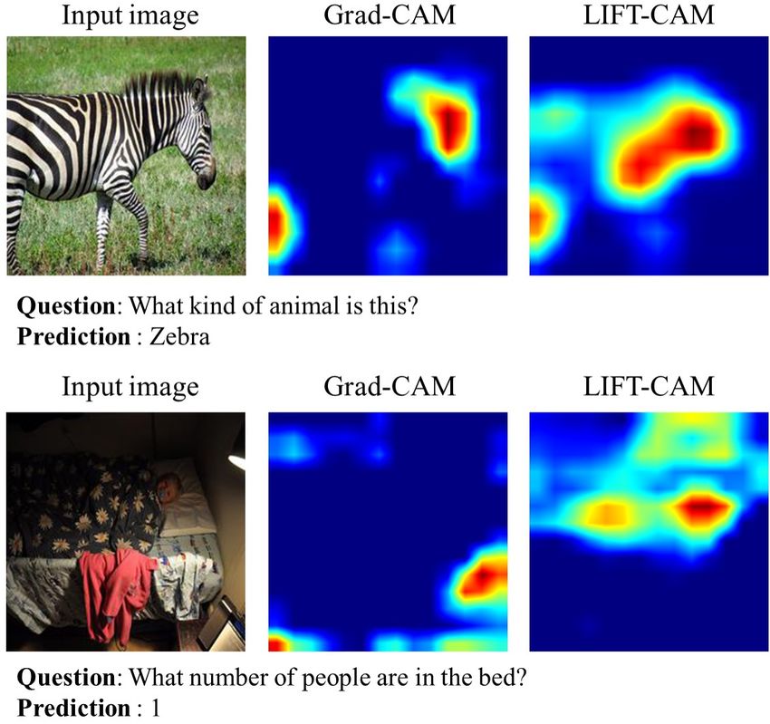
• We formulate the SHAP values of the activation maps               2.2. SHapley Additive exPlanations
     as a unified solution for the suggested framework. Fur-
                                                                       Additive feature attribution method. SHAP [11] is a uni-
     thermore, we verify the excellence of the values.
                                                                       fied explanation framework for the class of additive feature
   • We introduce a new saliency method, LIFT-CAM,                     attribution methods. The additive feature attribution method
     employing DeepLIFT. The method can estimate the                   follows:
                                                                                                         M
     SHAP values of the activation maps precisely. It out-                                   0          X       0
                                                                                          g(z ) = φ0 +      φi zi                (2)
     performs previous CAMs qualitatively and quantita-
                                                                                                          i=1
     tively by providing reliable visual explanations with a
                                                                       where g is an explanation model of an original prediction
     single backward propagation.
                                                                       model f and M is the number of features. φi denotes an
2. Related works                                                       importance of the i-th feature and φ0 is a baseline explana-
                                                                               0
                                                                       tion. z ∈ {0, 1}M indicates a binary vector in which each
2.1. CAM-based methods                                                 entry represents the existence of the corresponding original
Visual explanation map. Let f be an original prediction                feature; 1 for presence and 0 for absence. The methods are
                                                                                                0            0              0      0

model and c denote a target class of interest. CAMs [21,               designed to ensure g(z ) ≈ f (hx (z )) whenever z ≈ x ,
                                                                                                                                 0

15, 4, 19, 5, 8] aim to explain the target output of the model         with a mapping function hx which satisfies x = hx (x ).
for a specific input image x (i.e., f c (x)) through the visual        While several existing attribution methods [13, 3, 17, 10]
explanation map, which can be generated by:                            match Eq. (2), only one explanation model in the class sat-
                                                                       isfies the three desirable properties: local accuracy, miss-
                                      Nl
                                      X                                ingness, and consistency [11].
              LcCAM (A) = ReLU (            αk Ak )         (1)        SHAP values. A feature attribution of the explanation
                                      k=1                              model which obeys Eq. (2) while adhering to the above
                                                                       three properties is defined as SHAP values [11] and can be
with A = f [l] (x), where f [l] denotes the output of the l-th
                                                                       formulated by:
layer. Ak is a k-th activation map of A and αk is a cor-
responding weight coefficient (i.e., an importance) of Ak ,                   X (M − |z 0 | − 1)!|z 0 |!          0             0

respectively. Nl indicates the number of activation maps               φi =                              [f (hx (z )) − f (hx (z \i))]
                                                                              0 0
                                                                                       M    !
for layer l. This concept of linearly combining activation                    z ⊂x
                                                                                                                                  (3)
maps was firstly proposed by [21], leading to its variants.                       0                                            0
                                                                       where |z | denotes the number of non-zero entries of z and
Previous methods. Grad-CAM [15] decides the coefficient                  0      0                 0
                                                                       z ⊂ x represents all z vectors, where the non-zero en-
of a specific activation map by averaging the gradients over                                                          0
                                                                       tries are a subset of the non-zero entries in x . In addition,
all activation neurons in that map. Grad-CAM++ [4], which                0              0
                                                                       z \i indicates zi = 0. This definition of the SHAP values
is a modified version of Grad-CAM, focuses on positive
                                                                       intimately aligns with the classic Shapley values [16].
influences of neurons considering higher-order derivatives.
However, the gradients of deep neural networks tend to di-             2.3. DeepLIFT
minish due to the gradient saturation problem. Hence, using
                                                                          DeepLIFT [17] focuses on the difference between an
the unmodified raw gradients induces failure of localization
                                                                       original activation and a reference activation. It propagates
for relevant regions.
                                                                       the difference through a network to assign the contribution
    To overcome this limitation, gradient-free CAMs have
                                                                       score to each input neuron by linearizing non-linear compo-
been proposed. Score-CAM [19] overlaps normalized ac-
                                                                       nents in the network. Through this technique, the gradient
tivation maps to an input image and makes predictions to
                                                                       saturation problem is stabilized.
acquire the coefficients. Ablation-CAM [5] defines a coef-
                                                                          Let o represent the output of the target neuron and x =
ficient as the fraction of decline in the target output when the
                                                                       (x1 , . . . , xn ) be input neurons whose reference values are
associated activation map is removed. The two CAMs are
                                                                       r = (r1 , . . . , rn ). The contribution score of the i-th input
free from the saturation issues, but they are time-consuming
                                                                       feature C∆xi ∆o quantifies the influence of ∆xi = xi − ri
because they require Nl forward propagations to acquire the
                                                                       on ∆o = f (x) − f (r). In addition, DeepLIFT satisfies the
coefficients.
                                                                       summation-to-delta property as below:
    All the methods described above evaluate their coeffi-
                                                                                            n
cients in a heuristic way. XGrad-CAM [8] addresses this is-                                 X
sue by suggesting two axioms. The authors mathematically                                          C∆xi ∆o = ∆o.                    (4)
                                                                                            i=1
proved that the coefficients satisfying the axioms converge
to the summations of the “input×gradient” values of the ac-            Note that if we set C∆xi ∆o = φi and f (r) = φ0 , then Eq.
tivation neurons. However, their derivation is demonstrated            (4) matches Eq. (2). Therefore, DeepLIFT is also an ad-
only for ReLU-CNN.                                                     ditive feature attribution method for which the contribution

                                                                   2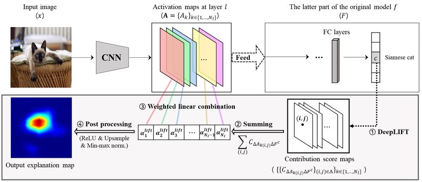
scores are among the solutions for Eq. (2). It approximates
the SHAP values efficiently, satisfying the local accuracy
and missingness [11].

3. Proposed Methodology
   In this section, we clarify the problem formulation of
CAM and suggest an approach to resolve it analytically.
First, we suggest a framework that defines a linear expla-
nation model and decides the weight coefficients of CAM
based on that model. Then, we formulate the SHAP val-
ues of the activation maps as a unified solution for the
model. Finally, we introduce a fast and precise approxi-               Figure 1. The suggested framework for determining the weight
mation method for the SHAP values using DeepLIFT.                      coefficients for CAM. First, we build a linear explanation model.
                                                                       Next, we determine the importance scores of activation maps by
3.1. Problem formulation of CAM                                        optimizing the explanation model based on additive feature attri-
                                                                       bution methods. Last, we convey the scores as the coefficients for
     As identified in Eq. (1), CAM produces a visual ex-               CAM.
planation map LcCAM linearly w.r.t. the activation maps
{Ak }k∈{1,...,N l } except for ReLU, which is applied for the
purpose of only considering the positive influence on the
target class c. In addition, the matrix of the complete ac-
                                                                       3.3. SHAP values of activation maps
tivation maps A = {Ak }k∈{1,...,N l } does not change for
                                                                           Next, we define the SHAP values of activation maps. Let
a given pair of the input image x and the model f . Thus,
                                                                       F be a latter part of the original model f , from layer l + 1
the responsibility of LcCAM is controlled by the weight co-
                                                                       to layer L − 11 , where L represents the total number of
efficients {αk }k∈{1,...,N l } , which represent the importance
                                                                       layers in f . Namely, we have F (A) = f [L−1] (x). Addi-
scores of the associated activation maps. To summarize,                                                                             0
                                                                       tionally, we define a mapping function hA that converts a
the purpose of CAM is to find the optimal coefficients
                                                                       into the embedding space of the activation maps: it satisfies
{αkopt }k∈{1,...,N l } for a linear combination in order to gen-                     0           0
                                                                       A = hA (A ), where A is a vector of ones. Specifically,
erate LcCAM , which can reliably explain the target output               0                               0
                                                                       ak = 1 is mapped to Ak and ak = 0 to 0, which has the
f c (x).
                                                                       same dimension as Ak . Note that this is reasonable because
3.2. The suggested framework                                           an activation map exerts no influence on visual explanation
                                                                       when it has values of 0 for all activation neurons in Eq. (1).
   How can we acquire the desirable coefficients in an an-
alytic way? To this end, we first consider each activation                Now, the SHAP values of the activation maps w.r.t. the
map as an individual feature (i.e., we have Nl features) and           class c can be formulated by [11]:
                          0
define a binary vector a ∈ {0, 1}Nl of the features. In
                      0
the vector, an entry ak of 1 indicates that the corresponding                       X (Nl − |a0 | − 1)!|a0 |!            0             0
activation map Ak maintains its original activation values,            αksh =                                 [F c (hA (a ))−F c (hA (a \k))]
                                                                                              N  l !
and 0 means that it loses the values. Next, we specify an                           0 0
                                                                                   a ⊂A
explanation model of CAM gCAM to interpret f c (x).                                                                              (6)
   Since the explanation map of CAM LcCAM is linear w.r.t.             where αksh is the SHAP value of the k-th activation map.
the activation maps A by definition, it is rational to assume          The above equation implies that αksh can be obtained by av-
that the explanation model gCAM is also linear w.r.t. the              eraging marginal prediction differences between presence
                                           0
binary variables of the activation maps a as follows:                  and absence of Ak across all possible feature orderings. In
                                                                       this context, Algorithm 1 shows the overall procedure to
                                     Nl
                         0           X         0                       approximate the SHAP values from a set of sampled order-
               gCAM (a ) = α0 +            αk ak .          (5)        ings. We refer to the approximation from |Π| orderings as
                                     k=1
                                                                       SHAP-CAM|Π| throughout the paper. The higher |Π|, the
This linear explanation model can be solved by the class               closer SHAP-CAM|Π| approximates {αksh }k∈{1,...,N l } . We
of additive feature attribution methods, matching Eq. (2)              validate the effectiveness and the superiority of these SHAP
perfectly. Therefore, the SHAP values can be adopted as                attributions in our experimental section.
a unified solution for {αk }k∈{1,...,N l } (see the supplemen-
tary materials for comparison with LIME [13]). Figure 1
represents the framework which is described in this section.              1 It   represents the logit layer which precedes the softmax layer.

                                                                   3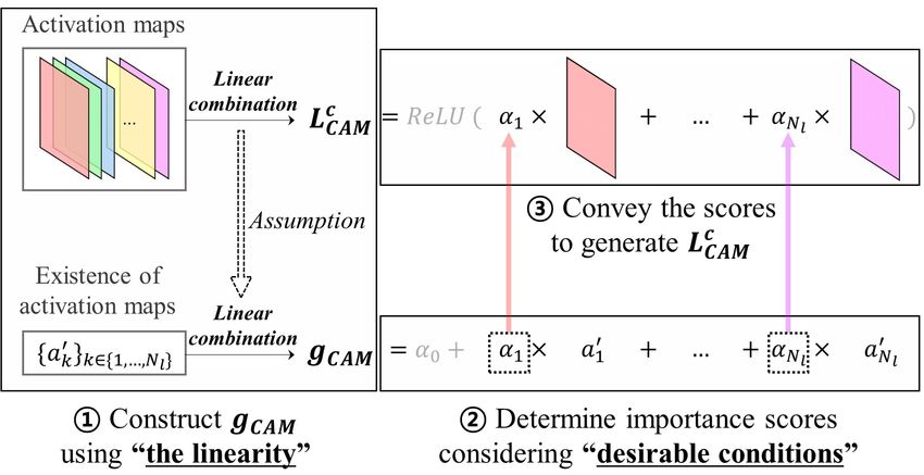
Figure 2. An overview of LIFT-CAM. First, we conduct DeepLIFT from the target output towards the activation maps and acquire the
contribution score maps, for which each pixel presents C∆Ak (i,j) ∆F c . Next, we quantify the importance of each activation map by
summing all the contribution scores of itself. Then, we perform a linear combination of {αklif t }k∈{1,...,Nl } and {Ak }k∈{1,...,Nl } . Finally,
we rectify the resulting map, upsample the map to the original image dimension, and normalize the map using the min-max normalization
function.

Algorithm 1 SHAP-CAM|Π| approximation                                           vation neuron through a single backward pass. Consider-
Input : F , c, hA , and a set of orderings Π of {1, · · · , Nl }                ing the summation-to-delta property of DeepLIFT, we de-
Output: {αk }k∈{1,...,Nl }                                                      fine the contribution score of the specific activation map as
Initialize: {αk }k∈{1,...,Nl } ←
                               −0                                               the summation of the contribution scores of all neurons in
for each ordering π in Π do                                                     that activation map, as follows:
     0
    a ← −0                                                                                                            X
    for i = 1, ..., Nl do                                                                    αklif t = C∆Ak ∆F c =             C∆Ak (i,j) ∆F c   (7)
          0
                                                                                                                     (i,j)∈Λ
        aπ(i) ←
              −1
                                          0                  0
       απ(i) ← − απ(i) + F c (hA (a )) − F c (hA (a \π(i)))                     where Λ = {1, . . . , H} × {1, . . . , W } is a discrete acti-
   end                                                                          vation dimension and Ak(i,j) is an activation value at the
end                                                                             (i, j) location of Ak . Note that ∆ denotes the difference-
{αk }k∈{1,...,Nl } ←
                   − {αk }k∈{1,...,Nl } /|Π|                                    from-reference and the reference values (i.e., uninformative
                                                                                values) of all activation neurons are set to 0, aligning with
                                                                                SHAP. By this definition, {αklif t }k∈{1,...,N l } becomes a re-
3.4. Efficient approximation: LIFT-CAM
                                                                                liable solution for Eq. (5) while satisfying the local accu-
   Through the experiment, we prove that a favorable vi-                        racy3 and the missingness as below:
sual explanation map can be achieved by the SHAP val-
                                                                                                   Nl
ues. However, calculating the exact SHAP values is almost                                          X
impossible. Therefore, we should consider an approxima-                                                  αklif t = F c (A) − F c (0).            (8)
tion approach. In this study, we propose a novel method,                                           k=1

LIFT-CAM, that efficiently approximates the SHAP values
                                                                                Using these DeepLIFT attributions, LIFT-CAM can esti-
of the activation maps using DeepLIFT2 [17] (see the sup-
                                                                                mate the SHAP values of the activation maps with a sin-
plementary materials for analysis of other approximation al-
                                                                                gle backward pass while alleviating the gradient saturation
gorithms).
                                                                                problem. Figure 2 shows an overview of our suggested
   First, we calculate the contribution score for every acti-                   LIFT-CAM. Additionally, the following two rationales mo-
   2 DeepLIFT-Rescale is adopted for approximation because the method           tivate us to employ DeepLIFT for this problem.
can be easily implemented by overriding gradient operators. This conve-               P Nl
nience enables LIFT-CAM to be easily applied to a large variety of tasks.         3
                                                                                        k=1   αsh   c       c
                                                                                               k = F (A) − F (0).

                                                                            4
1. DeepLIFT linearizes non-linear components to esti- SHAP values as the coefficients for CAM in Sec. 4.1. Then,
mate the SHAP values. Therefore, DeepLIFT attri- we demonstrate how closely LIFT-CAM can estimate the
butions tend to deviate from the true SHAP values SHAP values in Sec. 4.2. These two experiments provide
in the case of passing through many overlapped non- justification to opt for LIFT-CAM as a responsible method
linear layers during back-propagation (see the supple- of determining the coefficients for CAM. We then evaluate
mentary materials). However, for CAM, only the non- the performance of LIFT-CAM on the object recognition
linearities in F matter. Since CAM usually adopts task in the context of image classification, comparing it with
the outputs of the last convolutional layer as its acti- current state-of-the-art CAMs: Grad-CAM, Grad-CAM++,
vation maps, almost all F of state-of-the-art architec- Score-CAM, Ablation-CAM, and XGrad-CAM in Sec. 4.3.
tures contain few non-linearities (e.g., the VGG fam- Finally, we apply LIFT-CAM to the visual question answer-
ily), or are even fully linear (e.g., the ResNet family). ing (VQA) task in Sec. 4.4 to check the scalability of the
Thus, the SHAP values of the activation maps can be method.
approximated quite precisely (i.e., αlif t ≈ αsh ) by For all experiments except VQA, we employ the public
DeepLIFT. classification datasets ImageNet [14] (ILSVRC 2012 vali-
dation set), PASCAL VOC [6] (2007 test set), and COCO
2. The reference value (i.e., the value of the absent fea-
[9] (2014 validation set). In addition, the VGG16 net-
ture) should be defined as an uninformative value. For
work trained on each dataset is analyzed for the experi-
this problem, the reference values of all activation neu-
ments (see the supplementary materials for the experiments
rons are definitely 0 because the value cannot influence
of ResNet50). We refer to the pretrained models from the
LcCAM . This removes the need to heuristically choose
torchvision4 package for ImageNet and the TorchRay pack-
the reference values and enables acquisition of the ex-
age5 for VOC and COCO. For VQA, we adopt a fundamen-
act SHAP values using LIFT-CAM (i.e., αlif t = αsh )
tal architecture6 proposed by [2] and a typical VQA dataset7
for the architectures with linear F .
which is established on the basis of COCO [9].
3.5. Rethinking Ablation-CAM and XGrad-CAM
4.1. Validation for SHAP values
The recently proposed Ablation-CAM [5] and XGrad-
Evaluation metrics. Intuitively, an explanation image w.r.t.
CAM [8] can be reinterpreted by our framework. Ablation-
the target class c can be generated using an original image
CAM defines the coefficients as below:
0 0
x and a related visual explanation map LcCAM as below:
αkab = F c (h(A )) − F c (h(A \k)). (9)
ec = s(u(LcCAM )) ◦ x (11)
By adopting this specific marginal change as the coefficient,
Ablation-CAM can be deemed as another approximation where u(·) indicates the upsampling operation into the orig-
method for the SHAP values. Meanwhile, the coefficients inal input dimension and s(·) denotes a min-max normaliza-
of XGrad-CAM can be achieved by: tion function. The operator ◦ refers to the Hadamard prod-
X ∂F c (A) uct. Hence, ec preserves the information of x only in the
αkxg = Ak(i,j) × . (10) region which LcCAM considers important.
∂Ak(i,j)
(i,j)∈Λ In general, LcCAM is expected to recognize the regions
[1] proved that this “input×gradient” attribution is equiv- which contribute the most to the model’s decision. Thus, we
alent to the relevance score of layer-wise relevance prop- can evaluate the faithfulness of LcCAM on the object recog-
agation (LRP) [3] for ReLU-CNN. Therefore, αkxg can be nition task via the two metrics proposed in [4]: increase in
viewed as summing the relevance scores of the activation confidence (IIC) and average drop (AD), which are defined
neurons in the k-th activation map, similar to the approach as:
N
in LIFT-CAM. LRP is also an additive feature attribution 1 X
1[YicEvaluation metric Increase in confidence (%) Average drop (%) Average drop in deletion (%)
Dataset ImageNet VOC COCO ImageNet VOC COCO ImageNet VOC COCO
SHAP-CAM1 25.9 37.4 35.2 28.16 22.93 23.98 32.64 17.35 24.07
SHAP-CAM10 26.2 42.7 40.1 27.54 17.53 19.07 32.99 19.95 27.50
SHAP-CAM100 26.4 43.6 41.4 27.48 16.71 18.27 33.03 20.64 27.65
Table 1. Faithfulness evaluation on the object recognition task. We analyze 1,000 randomly selected images for each dataset. Higher is
better for the increase in confidence and average drop in deletion. Lower is better for the average drop.
eci , accordingly. N denotes the number of images and 1[·] is ImageNet VOC COCO
an indicator function. Higher is better for IIC and lower is Grad-CAM 0.489 0.404 0.441
better for AD. Grad-CAM++ 0.385 0.329 0.412
However, IIC and AD evaluate the performance of the Score-CAM 0.195 0.181 0.157
explanations via the preservation perspective; the region Ablation-CAM 0.972 0.888 0.908
which is considered to be influential is maintained. We can XGrad-CAM 0.969 0.865 0.877
also evaluate the performance using the opposite perspec- LIFT-CAM 0.980 0.918 0.924
tive (i.e., deletion); if we mute the region which is responsi-
ble for the target output, the softmax probability is expected Table 2. The cosine similarities between the coefficients from
to significantly drop. From this viewpoint, we suggest aver- CAMs and those from SHAP-CAM10k . We randomly choose 500
age drop in deletion (ADD) which can be defined as below: images from each dataset for analysis.
N
1 X (Yic − Dic ) the justification of this assumption). Table 2 shows the co-
× 100 (14)
N i=1 Yic sine similarities between the coefficients from state-of-the-
art CAMs, including LIFT-CAM, and those from SHAP-
where Dc is the softmax output of the inverted explanation CAM10k . The similarity is averaged over 500 randomly se-
map ecinv = (1 − s(u(LcCAM ))) ◦ x. Higher is better for lected images for each dataset.
this metric. As shown in Table 2, LIFT-CAM presents the highest
Faithfulness evaluation. Table 1 presents the comparative similarities for all datasets (greater than 0.9), which in-
results of IIC, AD, and ADD for SHAP-CAM1 , SHAP- dicates high relevance between the importance scores in
CAM10 , and SHAP-CAM100 . We analyze 1,000 randomly LIFT-CAM and the SHAP values. Even if Ablation-CAM
selected images for each dataset. Furthermore, each case is and XGrad-CAM also exhibit high similarities, they fall be-
averaged over 10 simulations for fair comparison. We can hind LIFT-CAM due to dissatisfaction of the local accuracy
discover two important implications from Table 1. First, property. The other CAMs cannot approximate the SHAP
as the number of orderings increases, IIC and ADD in- values, providing consistently low similarities.
crease and AD decreases, showing performance improve-
ment. This result indicates that the closer the importance 4.3. Performance evaluation of LIFT-CAM
of the activation map is to the SHAP value, the more ef- The experimental results from Secs. 4.1 and 4.2 moti-
fectively the distinguishable region of the target object is vate us to evaluate the importances of activation maps with
found. Second, even compared to the other CAMs (see Ta- LIFT-CAM. To confirm the excellence of our LIFT-CAM,
ble 3), SHAP-CAM100 shows the best performances for all we compare the performances of the method with those of
cases. It reveals the superiority of the SHAP attributions as various state-of-the-art saliency methods.
the weight coefficients for CAM. However, this approach of
averaging the marginal contributions of multiple orderings
4.3.1 Qualitative evaluation
is impractical due to the significant computational burden.
Therefore, we propose a cleverer approximation method: Figure 3 provides qualitative comparisons between various
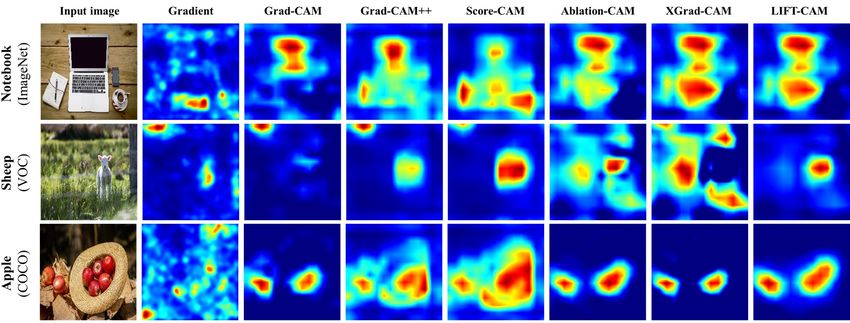
LIFT-CAM. saliency methods via visualization. Each row represents
the visual explanation maps for each dataset. When com-
4.2. Approximation performance of LIFT-CAM
pared to the other methods, our proposed method, LIFT-
In this section, we quantitatively assess how precisely CAM, yields visually interpretable explanation maps for all
LIFT-CAM estimates the SHAP values of the activation cases. It clearly pinpoints the essential parts of the specific
maps. Since the exact SHAP values are unattainable, we objects which are responsible for the classification results.
regard the coefficients from SHAP-CAM10k as the true val- This can be noted in the notebook case (row 1), for which
ues for comparison (see the supplementary materials for most of the other visualizations cannot decipher the lower
6Figure 3. Visual explanation maps of state-of-the-art saliency methods and our proposed LIFT-CAM. Note that we apply a smoothing
technique [7] to Gradient [18] to acquire plausible explanation maps.
Evaluation metric Increase in confidence (%) Average drop (%) Average drop in deletion (%)
Dataset ImageNet VOC COCO ImageNet VOC COCO ImageNet VOC COCO
Grad-CAM 24.0 32.7 31.9 31.89 30.73 30.74 30.60 17.43 25.66
Grad-CAM++ 23.1 33.8 33.5 30.53 17.20 20.87 27.98 15.85 24.16
Score-CAM 22.8 29.4 23.9 29.91 17.49 23.66 27.52 14.12 17.35
Ablation-CAM 24.1 34.4 35.0 29.41 25.49 23.99 32.52 19.42 26.75
XGrad-CAM 24.7 31.7 32.5 29.19 29.52 28.52 27.52 19.00 26.09
LIFT-CAM 25.2 38.7 39.3 29.15 17.15 18.65 32.95 20.09 26.34
Table 3. Comparative evaluation of faithfulness on the object recognition task among various CAMs. Results with 1,000 randomly sampled
images are provided for each dataset. Higher is better for the increase in confidence and average drop in deletion. Lower is better for the
average drop.
part of the notebook. Furthermore, LIFT-CAM alleviates Insertion Deletion
pixel noise without highlighting trivial evidence. In the Grad-CAM 0.4427 0.0891
sheep case (row 2), the artifacts of the image are eliminated Grad-CAM++ 0.4350 0.0969
by LIFT-CAM and the exact location of the sheep is cap- Score-CAM 0.4345 0.1002
tured by the method. Last, the method successfully locates Ablation-CAM 0.4685 0.0873
multiple objects in the apple case (row 3) by providing the XGrad-CAM 0.4680 0.0871
object-focused map. LIFT-CAM 0.4712 0.0866
Table 4. The AUC results in terms of insertion and deletion. The
4.3.2 Faithfulness evaluation values are averaged over 1,000 randomly selected images from
ImageNet. Higher is better for insertion and lower is better for
IIC, AD, and ADD. Table 3 shows the results of IIC, AD, deletion.
and ADD of each CAM in various datasets. The three met-
rics can represent the object recognition performances of
the saliency methods in a complementary way. LIFT-CAM can accurately and efficiently determine which object is re-
provides the best results in most cases. Exceptionally, for sponsible for the model’s prediction.
ADD in COCO, Ablation-CAM presents a better result than Area under probability curve. The above three metrics
LIFT-CAM. However, LIFT-CAM also provides a compa- tend to be advantageous for methods which provide expla-
rable result, exhibiting the negligible difference. In addi- nation maps of large magnitude. To exclude the influence
tion, it should be noted that LIFT-CAM is much faster than of the magnitude, we can binarize the explanation map with
Ablation-CAM since it requires only a single backward pass two opposite perspectives: insertion and deletion [12]. We
to calculate the coefficients. In consequence, LIFT-CAM simply introduce or remove pixels from an image by setting
7Grad-CAM Grad-CAM++ Score-CAM Ablation-CAM XGrad-CAM LIFT-CAM
Proportion (%) 47.76 49.14 51.14 51.87 51.85 52.43
Table 5. The proportions of energy located in bounding boxes for various CAMs. The values are averaged over 1,000 randomly selected
images from ImageNet.
the pixel values of the explanation map to one or zero with
step 0.025 (introduce or remove 2.5% pixels of the whole
image in each step) and calculate the area under the proba-
bility curve (AUC). As shown in Table 4, LIFT-CAM pro-
vides the most reliable results, presenting the highest inser-
tion AUC and the lowest deletion AUC. Through this exper-
iment, we confirm that LIFT-CAM succeeds in sorting the
pixels according to the contributions to the target result.
4.3.3 Localization evaluation
It is reasonable to expect that a dependable explanation map
overlaps with a target object. Therefore, we can also assess
the reliability of the map via localization ability in addition
to the softmax probability. [19] proposed a new localiza-
tion metric, the energy-based pointing game, which is an
improved version of the pointing game [20]. The metric
gauges how much energy of the explanation map interacts
with the bounding box of the target object. The metric can
be formulated as follows: Figure 4. Visual explanation maps of Grad-CAM and LIFT-CAM
for VQA.
c
P
(i,j)∈bbox s(u(LCAM ))(i,j)
Proportion = P (15)
c
(i,j)∈Λ0 s(u(LCAM ))(i,j)
Grad-CAM LIFT-CAM
Increase in confidence (%) 41.95 43.39
0 0 0
where Λ = {1, . . . , H } × {1, . . . , W } is an original im- Average drop (%) 16.71 14.14
age dimension. Therefore, s(u(LcCAM ))(i,j) denotes a min- Average drop in deletion (%) 9.09 9.58
max normalized importance at pixel location (i, j).
The proportions of the various methods are reported in Table 6. Faithfulness evaluation for the VQA task. The values
are computed through the complete validation sets (214,354 image
Table 5. LIFT-CAM shows the highest proportion com-
and question pairs). Higher is better for the increase in confidence
pared to the other methods. This implies that LIFT-CAM
and average drop in deletion. Lower is better for the average drop.
produces a compact explanation map which focuses on the
essential parts of the images with less noise.
comparison results between Grad-CAM and LIFT-CAM in
4.4. Application to VQA
terms of those metrics. As demonstrated in the table, LIFT-
We also apply LIFT-CAM to VQA to demonstrate the CAM provides performances superior to Grad-CAM for all
applicability of the method. We consider the standard VQA of the metrics. This indicates that LIFT-CAM is better at
model [2] which consists of a CNN and a recurrent neu- figuring out the essential parts of images, which can serve
ral network in parallel. They function to embed images as evidence for the answers to the questions.
and questions, respectively. The two embedded vectors are
fused and entered into a classifier to produce the answer. 5. Conclusion
Figure 4 illustrates the explanation maps of Grad-CAM
and LIFT-CAM. As displayed in the figure, LIFT-CAM suc- In this work, we suggest a novel analytic framework to
ceeds in highlighting the regions in the given images which decide the weight coefficients of CAM using additive fea-
are more relevant to the question and prediction pairs than ture attribution methods. Based on the idea that SHAP
Grad-CAM. Additionally, since this is a classification prob- values is a unified solution of the methods, we adopt the
lem, the IIC, AD, and ADD of each method can be evalu- values as the coefficients and demonstrate their excellence.
ated with fixed question embeddings. Table 6 represents the Moreover, we introduce LIFT-CAM, which approximates
8the SHAP values of activation maps precisely with a single [13] Marco Tulio Ribeiro, Sameer Singh, and Carlos Guestrin.
backward pass. It presents quantitatively and qualitatively ” why should i trust you?” explaining the predictions of any
enhanced visual explanations compared with the other pre- classifier. In Proceedings of the 22nd ACM SIGKDD interna-
vious CAMs. tional conference on knowledge discovery and data mining,
pages 1135–1144, 2016.
References [14] Olga Russakovsky, Jia Deng, Hao Su, Jonathan Krause, San-
jeev Satheesh, Sean Ma, Zhiheng Huang, Andrej Karpathy,
[1] Marco Ancona, Enea Ceolini, Cengiz Öztireli, and Markus Aditya Khosla, Michael Bernstein, et al. Imagenet large
Gross. Towards better understanding of gradient-based attri- scale visual recognition challenge. International journal of
bution methods for deep neural networks. In International computer vision, 115(3):211–252, 2015.
Conference on Learning Representations, 2018. [15] Ramprasaath R Selvaraju, Michael Cogswell, Abhishek Das,
[2] Stanislaw Antol, Aishwarya Agrawal, Jiasen Lu, Margaret Ramakrishna Vedantam, Devi Parikh, and Dhruv Batra.
Mitchell, Dhruv Batra, C Lawrence Zitnick, and Devi Parikh. Grad-cam: Visual explanations from deep networks via
Vqa: Visual question answering. In Proceedings of the IEEE gradient-based localization. In Proceedings of the IEEE in-
international conference on computer vision, pages 2425– ternational conference on computer vision, pages 618–626,
2433, 2015. 2017.
[3] Sebastian Bach, Alexander Binder, Grégoire Montavon, [16] Lloyd S Shapley. A value for n-person games. Technical
Frederick Klauschen, Klaus-Robert Müller, and Wojciech report, Rand Corp Santa Monica CA, 1952.
Samek. On pixel-wise explanations for non-linear classi- [17] Avanti Shrikumar, Peyton Greenside, and Anshul Kundaje.
fier decisions by layer-wise relevance propagation. PloS one, Learning important features through propagating activation
10(7):e0130140, 2015. differences. In International Conference on Machine Learn-
[4] Aditya Chattopadhay, Anirban Sarkar, Prantik Howlader, ing, pages 3145–3153, 2017.
and Vineeth N Balasubramanian. Grad-cam++: General- [18] K. Simonyan, A. Vedaldi, and Andrew Zisserman. Deep in-
ized gradient-based visual explanations for deep convolu- side convolutional networks: Visualising image classifica-
tional networks. In 2018 IEEE Winter Conference on Appli- tion models and saliency maps. CoRR, abs/1312.6034, 2014.
cations of Computer Vision (WACV), pages 839–847. IEEE,
[19] Haofan Wang, Zifan Wang, Mengnan Du, Fan Yang, Zijian
2018.
Zhang, Sirui Ding, Piotr Mardziel, and Xia Hu. Score-cam:
[5] Saurabh Desai and Harish G Ramaswamy. Ablation-cam:
Score-weighted visual explanations for convolutional neural
Visual explanations for deep convolutional network via
networks. In Proceedings of the IEEE/CVF Conference on
gradient-free localization. In 2020 IEEE Winter Conference
Computer Vision and Pattern Recognition Workshops, pages
on Applications of Computer Vision (WACV), pages 972–
24–25, 2020.
980. IEEE, 2020.
[20] Jianming Zhang, Sarah Adel Bargal, Zhe Lin, Jonathan
[6] Mark Everingham, Luc Van Gool, Christopher KI Williams,
Brandt, Xiaohui Shen, and Stan Sclaroff. Top-down neu-
John Winn, and Andrew Zisserman. The pascal visual object
ral attention by excitation backprop. International Journal
classes (voc) challenge. International journal of computer
of Computer Vision, 126(10):1084–1102, 2018.
vision, 88(2):303–338, 2010.
[21] Bolei Zhou, Aditya Khosla, Agata Lapedriza, Aude Oliva,
[7] Ruth Fong, Mandela Patrick, and Andrea Vedaldi. Un-
and Antonio Torralba. Learning deep features for discrimina-
derstanding deep networks via extremal perturbations and
tive localization. In Proceedings of the IEEE conference on
smooth masks. In Proceedings of the IEEE International
computer vision and pattern recognition, pages 2921–2929,
Conference on Computer Vision, pages 2950–2958, 2019.
2016.
[8] Ruigang Fu, Qingyong Hu, Xiaohu Dong, Yulan Guo,
Yinghui Gao, and Biao Li. Axiom-based grad-cam: To-
wards accurate visualization and explanation of cnns. In 31th
British Machine Vision Conference, BMVC 2020.
[9] Tsung-Yi Lin, Michael Maire, Serge Belongie, James Hays,
Pietro Perona, Deva Ramanan, Piotr Dollár, and C Lawrence
Zitnick. Microsoft coco: Common objects in context. In
European conference on computer vision, pages 740–755.
Springer, 2014.
[10] Stan Lipovetsky and Michael Conklin. Analysis of regres-
sion in game theory approach. Applied Stochastic Models in
Business and Industry, 17(4):319–330, 2001.
[11] Scott M Lundberg and Su-In Lee. A unified approach to
interpreting model predictions. In Advances in neural infor-
mation processing systems, pages 4765–4774, 2017.
[12] Vitali Petsiuk, Abir Das, and Kate Saenko. Rise: Random-
ized input sampling for explanation of black-box models. In
29th British Machine Vision Conference, BMVC 2018.
9You can also read