Robust Imitation Learning from Noisy Demonstrations
←
→
Page content transcription
If your browser does not render page correctly, please read the page content below
Robust Imitation Learning from Noisy Demonstrations

                                                    Voot Tangkaratt                Nontawat Charoenphakdee                 Masashi Sugiyama
                                                         RIKEN                      University of Tokyo & RIKEN         RIKEN & University of Tokyo
                                                voot.tangkaratt@riken.jp           nontawat@ms.k.u-tokyo.ac.jp            sugi@k.u-tokyo.ac.jp
arXiv:2010.10181v3 [stat.ML] 19 Feb 2021

                                                                Abstract                             In the literature, methods for IL from noisy demon-
                                                                                                     strations have been proposed, but they still have lim-
                                               Robust learning from noisy demonstrations             itations as they require additional labels from experts
                                               is a practical but highly challenging prob-           or a strict assumption about noise (Brown et al., 2019,
                                               lem in imitation learning. In this paper, we          2020; Wu et al., 2019; Tangkaratt et al., 2020). Specif-
                                               first theoretically show that robust imitation        ically, methods of Brown et al. (2019, 2020) require
                                               learning can be achieved by optimizing a clas-        noisy demonstrations to be ranked according to their
                                               sification risk with a symmetric loss. Based          relative performance. Meanwhile, methods of Wu
                                               on this theoretical finding, we then propose          et al. (2019) require some of noisy demonstrations to
                                               a new imitation learning method that op-              be labeled with a score determining the probability
                                               timizes the classification risk by effectively        that demonstrations are collected from experts. On
                                               combining pseudo-labeling with co-training.           the other hand, the method of Tangkaratt et al. (2020)
                                               Unlike existing methods, our method does              does not require these labels, but instead it assumes
                                               not require additional labels or strict assump-       that noisy demonstrations are generated by Gaussian
                                               tions about noise distributions. Experimen-           noise distributions. To sum up, these methods require
                                               tal results on continuous-control benchmarks          either additional labels from experts or a strict as-
                                               show that our method is more robust com-              sumption about noise distributions. Due to this, the
                                               pared to state-of-the-art methods.                    practicality of these methods is still limited, and IL
                                                                                                     from noisy demonstrations is still highly challenging.
                                                                                                     To overcome the above limitation, we propose a new
                                           1   INTRODUCTION                                          method for IL from noisy demonstrations called Ro-
                                                                                                     bust IL with Co-pseudo-labeling (RIL-Co). Briefly, we
                                           The goal of sequential decision making is to learn a      built upon the recent theoretical results of robust clas-
                                           good policy that makes good decisions (Puterman,          sification (Charoenphakdee et al., 2019), and prove
                                           1994). Imitation learning (IL) is an approach that        that robust IL can be achieved by optimizing a clas-
                                           learns a policy from demonstrations (i.e., sequences of   sification risk with a symmetric loss. However, op-
                                           demonstrators’ decisions) (Schaal, 1999). Researchers     timizing the proposed risk is not trivial because it
                                           have shown that a good policy can be learned ef-          contains a data density whose data samples are not
                                           ficiently from high-quality demonstrations collected      observed. We show that pseudo-labeling (Chapelle
                                           from experts (Ng and Russell, 2000; Ho and Ermon,         et al., 2010) can be utilized to estimate the data den-
                                           2016). However, demonstrations in the real-world of-      sity. However, naive pseudo-labeling may suffer from
                                           ten have lower quality due to noise or insufficient       over-fitting and is not suitable in practice (Kingma
                                           expertise of demonstrators, especially when humans        et al., 2014). To remedy this issue, we propose co-
                                           are involved in the data collection process (Mandlekar    pseudo-labeling, which effectively combines pseudo-
                                           et al., 2018). This is problematic because low-quality    labeling with co-training (Blum and Mitchell, 1998).
                                           demonstrations can reduce the efficiency of IL both in    Compare to prior work, RIL-Co does not require ad-
                                           theory and practice (Tangkaratt et al., 2020). In this    ditional labels or assumptions about noise distribu-
                                           paper, we theoretically and experimentally show that      tions. In addition, RIL-Co does not require an addi-
                                           IL can perform well even in the presence of noises.       tional hyper-parameter tuning because an appropriate
                                                                                                     hyper-parameter value can be derived from the theory.
                                                                                                     Experiments on continuous-control benchmarks show
                                                                                                     that RIL-Co is more robust against noisy demonstra-
                                                                                                     tions when compared to state-of-the-art methods.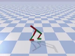
Robust Imitation Learning from Noisy Demonstrations
2 IMITATION LEARNING AND unavailable (Ng and Russell, 2000). Instead of learning
ROBUSTNESS from the reward function or reward values, IL methods
learn an optimal policy from demonstrations that con-
In this section, we firstly give backgrounds about rein- tain information about an optimal policy. IL methods
forcement learning and imitation learning. Then, we typically assume that demonstrations (i.e., a dataset of
describe the setting of imitation learning from noisy state-action samples) are collected by using an expert
demonstrations. Lastly, we discuss the robustness of policy that is similar to an optimal (or near optimal)
existing imitation learning methods. policy, and they aim to learn the expert policy (Ng and
Russell, 2000; Ziebart et al., 2010; Sun et al., 2019).
2.1 Reinforcement Learning More formally, the typical goal of IL is to learn an ex-
pert policy πE by using a dataset of state-action sam-
Reinforcement learning (RL) aims to learn an optimal ples drawn from an expert state-action density:
policy of a Markov decision process (MDP) (Puter- i.i.d.
man, 1994). We consider a discrete-time MDP denoted tpsn , an quN
n“1 „ ρE ps, aq, (2)
by M “ pS, A, pT ps1 |s, aqq, p1 ps1 q, rps, aq, γq with state
where ρE is a state-action density of expert policy πE .
s P S, action a P A, transition probability density pT ,
initial state probability density p1 , reward function r, The density matching approach was shown to be effec-
and discount factor 0 ă γ ď 1. A policy function tive in learning the expert policy from expert demon-
πpa|sq determines the conditional probability density strations (Syed et al., 2008; Ho and Ermon, 2016;
of an action in a state. An agent acts in an MDP Ghasemipour et al., 2020). Briefly, this approach seeks
by observing a state, choosing an action according to for a policy π that minimizes a divergence between the
a policy, transiting to a next state according to the state-action densities of the expert and learning poli-
transition probability density, and possibly receiving cies. Formally, this approach aims to solve the follow-
an immediate reward according to the reward function. ing optimization problem:
An optimal policy of an MDP is a policy maximizing
the expected cumulative discounted rewards. min DpρE ps, aq||ρπ ps, aqq, (3)
π
Formally, RL seeks for an optimal policy by solving where D is a divergence such as the Jensen-Shannon
the optimization problem maxπ J pπq, where J pπq is divergence1 . In practice, the divergence, which con-
the expected cumulative discounted rewards defined as tains unknown state-action densities, is estimated by
”ř
T t´1
ı using demonstrations and trajectories drawn from ρE
J pπq “ Epπ t“1 γ rpst , at q and ρπ , respectively. A well-known density match-
“ Eρπ rrpst , at qs {p1 ´ γq. (1) ing method is generative adversarial IL (GAIL) (Ho
and Ermon, 2016), which minimizes an estimate of the
Here, pπ pτ q “ p1 ps1 qΠTt“1 pT pst`1 |st , at qπpat |st q is the Jensen-Shannon divergence by solving
probability density of trajectory τ “ ps1 , a1 , . . . , sT `1 q „ ˆ ˙
with length T , ρπ ps, aq “ p1 ´ γqEpπ pτ q rΣTt“1 γ t´1 δpst ´ 1
min max EρE log
s, at ´ aqs is the state-action density determining the π g 1 ` expp´gps, aqq
„ ˆ ˙
probability density of the agent with π observing s and 1
executing a, and δpst ´s, at ´aq is the Dirac delta func- ` Eρπ log , (4)
1 ` exppgps, aqq
tion. Note that the state-action density is a normal-
ized occupancy measure and uniquely corresponds to where g : S ˆ A ÞÑ R is a discriminator function.
a policy by
ş a relation πpa|sq “ ρπ ps, aq{ρπ psq, where Density matching methods were shown to scale well to
ρπ psq “ A ρπ ps, aqda (Syed et al., 2008). Also note high-dimensional problems when combined with deep
that the optimal policy is not necessarily unique since neural networks (Ho and Ermon, 2016; Ghasemipour
there can be different policies that achieve the same et al., 2020). However, an issue of this approach is
expected cumulative discounted rewards. that it is not robust against noisy demonstrations in
While RL has achieved impressive performance in re- general, as will be described in Section 2.4.
cent years (Silver et al., 2017), its major limitation is
that it requires a suitable reward function which may 2.3 Learning from Noisy Demonstrations
be unavailable in practice (Schaal, 1999).
In this paper, we consider a scenario of IL from
2.2 Imitation Learning noisy demonstrations, where given demonstrations are
1
For non-symmetric divergence, an optimization prob-
Imitation learning (IL) is a well-known approach to lem minπ Dpρπ ps, aq||ρE ps, aqq can be considered as
learn an optimal policy when the reward function is well (Ghasemipour et al., 2020).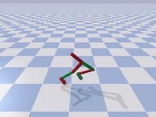
Voot Tangkaratt, Nontawat Charoenphakdee, Masashi Sugiyama

a mixture of expert and non-expert demonstrations.          demonstrations that are labeled with a score deter-
We assume that we are given a dataset of state-action       mining the probability that demonstrations are drawn
samples drawn from a noisy state-action density:            from ρE . However, this method is not applicable in our
                                i.i.d.                      setting since labeled demonstrations are not available.
             D “ tpsn , an quN      1
                             n“1 „ ρ ps, aq,         (5)
where the noisy state-action density ρ1 is a mixture of     3      ROBUST IMITATION LEARNING
the expert and non-expert state-action densities:
        ρ1 ps, aq “ αρE ps, aq ` p1 ´ αqρN ps, aq.   (6)    In this section, we propose our method for robust IL.
                                                            Briefly, in Section 3.1, we propose an IL objective
Here, 0.5 ă α ă 1 is an unknown mixing coefficient          which optimizes a classification risk with a symmet-
and ρN is the state-action density of a non-expert pol-     ric loss and prove its robustness. Then, in Section 3.2,
icy πN . The policy πN is non-expert in the sense that      we propose a new IL method that utilizes co-pseudo-
EρN rrps, aqs ă EρE rrps, aqs, where r is an unknown re-    labeling to optimize the classification risk. Lastly, we
ward function of the MDP. Our goal is to learn the          discuss the choice of a hyper-parameter in Section 3.3
expert policy using the dataset in Eq. (5).                 and the choice of symmetric losses in Section 3.4.
We emphasize that 0.5 ă α ă 1 corresponds to an as-
sumption that the majority of demonstrations are ob-        3.1      Imitation Learning via Risk Optimization
tained by the expert policy. This is a typical assump-
                                                            Classification risks are fundamental quantities in clas-
tion when learning from noisy data, i.e., the number of
                                                            sification (Hastie et al., 2001). We are interest in a
good quality samples should be more than that of low
                                                            balanced risk for binary classification where the class
quality samples (Angluin and Laird, 1988; Natarajan
                                                            prior is balanced (Brodersen et al., 2010). Specifically,
et al., 2013). For notational brevity, we denote a state-
                                                            we propose to perform IL by solving the following risk
action pair by x “ ps, aq, where x P X and X “ S ˆ A.
                                                            optimization problem:
2.4   Robustness of Imitation Learning                                         max min Rpg; ρ1 , ρλπ , `sym q,          (9)
                                                                                 π      g
It can be verified that the density matching approach
                                                            where R is the balanced risk defined as
is not robust against noisy demonstrations according
to the data generation assumption in Eq. (6). Specifi-                                 1                1
                                                                Rpg; ρ1 , ρλπ , `q “     Eρ1 r`pgpxqqs ` Eρλπ r`p´gpxqqs ,
cally, given demonstrations drawn from ρ1 , the density                                2                2
matching approach would solve minπ Dpρ1 pxq||ρπ pxqq.
By assuming that the space of π is sufficiently large,      and ρλπ is a mixture density defined as
the solution of this optimization problem is                               ρλπ pxq “ λρN pxq ` p1 ´ λqρπ pxq.          (10)
                     ˆ                         ˙
    ‹                          αρE pxq
  π pa|sq “ πE pa|sq                                        Here, 0 ă λ ă 1 is a hyper-parameter, π is a policy
                       αρE pxq ` p1 ´ αqρN pxq
                       ˆ                         ˙          to be learned by maximizing the risk, g : X ÞÑ R is
                              p1 ´ αqρN pxq                 a classifier to be learned by minimizing the risk, and
            ` πN pa|sq                             , (7)
                         αρE pxq ` p1 ´ αqρN pxq            `sym : R ÞÑ R is a symmetric loss satisfying
which yields Dpρ1 pxq||ρπ‹ pxqq “ 0. However, this pol-
                                                                            `sym pgpxqq ` `sym p´gpxqq “ c,            (11)
icy is not equivalent to the expert policy unless α “ 1.
Therefore, density matching is not robust against noisy     for all x P X , where c P R is a constant. Appro-
demonstrations generated according to Eq. (6).              priate choices of the hyper-parameter and loss will be
We note that the data generation assumption in              discussed in Sections 3.3 and 3.4, respectively.
Eq. (6) has been considered previously by Wu et al.         We note that the balanced risk assumes that the pos-
(2019). In this prior work, the authors proposed a          itive and negative class priors are equal to 21 . This
robust method that learns the policy by solving             assumption typically makes the balanced risk more re-
        min Dpρ1 pxq||αρπ pxq ` p1 ´ αqρN pxqq.      (8)    strictive than other risks, because a classifier is learned
         π                                                  to maximize the balanced accuracy instead of the ac-
The authors showed that this optimization problem           curacy (Menon et al., 2013; Lu et al., 2019). However,
yields the expert policy under the data generation as-      the balanced risk is not too restrictive for IL, because
sumption in Eq. (6). However, solving this optimiza-        the goal is to learn the expert policy and the classifier is
tion problem requires α and ρN which are typically un-      discarded after learning. Moreover, existing methods
known. To overcome this issue, Wu et al. (2019) pro-        such as GAIL can be viewed as methods that optimize
posed to estimate α and ρN by using additional noisy        the balanced risk, as will be discussed in Section 3.3.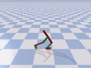
Robust Imitation Learning from Noisy Demonstrations

Next, we prove that the optimization in Eq. (9) yields            Proof sketch. It can be shown that the solution of
the expert policy under the following assumption.                 maxπ Rpg ‹´; ρ1 , ρλπ , `sym q is equivalent to the solution ¯
                                                                                                                               of
Assumption 1 (Mixture state-action density). The                  maxπ κpπq EρE r`sym p´g ‹ pxqqs´EρN r`sym p´g ‹ pxqqs .
state-action density of the learning policy π is a mix-           Since g ‹ “ argming Rpg; ρE , ρN , `sym q, it follows that
ture of the state-action densities of the expert and non-                       ‹                       ‹
expert policies with a mixing coefficient 0 ď κpπq ď 1:                      ´ pxqqs ´ EρN r`sym p´g pxqqs ą 0. Thus,
                                                                  EρE r`sym p´g                                            ¯
                                                                  maxπ κpπq EρE r`sym p´g ‹ pxqqs ´ EρN r`sym p´g ‹ pxqqs
      ρπ pxq “ κpπqρE pxq ` p1 ´ κpπqqρN pxq,            (12)     is solved by increasing κpπq to 1. Because κpπq “ 1
                                                                  if and only if ρπ pxq “ ρE pxq under Assumption 1, we
where ρπ pxq, ρE pxq, and ρN pxq are the state-action             conclude that the solution of maxπ Rpg ‹ ; ρ1 , ρλπ , `sym q
densities of the learning policy, the expert policy, and          is equivalent to the expert policy.
the non-expert policy, respectively.

This assumption is based on the following observation             A detailed proof is given in Appendix A. This result
on a typical optimization procedure of π: At the start            indicates that robust IL can be achieved by optimizing
of learning, π is randomly initialized and generates              the risk in Eq. (9). In a practice aspect, this is a
data that are similar to those of the non-expert policy.          significant advance compared to the prior work (Wu
This scenario corresponds to Eq. (12) with κpπq « 0.              et al., 2019), because Theorem 1 shows that robust IL
As training progresses, the policy improves and gener-            can be achieved without the knowledge of the mixing
ates data that are a mixture of those from the expert             coefficient α or additional labels to estimate α. Next,
and non-expert policies. This scenario corresponds to             we present a new IL method that empirically solves
Eq. (12) with 0 ă κpπq ă 1. Indeed, the scenario                  Eq. (9) by using co-pseudo-labeling.
where the agent successfully learns the expert policy
corresponds to Eq. (12) with κpπq “ 1.                            3.2     Co-pseudo-labeling for Risk Optimization

We note that a policy uniquely corresponding to ρπ                While the risk in Eq. (9) leads to robust IL, we can-
in Eq. (12) is a mixture between πE and πN with a                 not directly optimize this risk in our setting. This is
mixture coefficient depending on κpπq. However, we                because the risk contains an expectation over ρN pxq,
cannot directly evaluate the value of κpπq. This is               but we are given only demonstration samples drawn
because we do not directly optimize the state-action              from ρ1 pxq2 . We address this issue by using co-pseudo-
density ρπ . Instead, we optimize the policy π by using           labeling to approximately draw samples from ρN pxq, as
an RL method, as will be discussed in Section 3.2.                described below.
Under Assumption 1, we obtain Lemma 1.                            Recall that the optimal classifier g ‹ pxq in Eq. (14) also
Lemma 1. Letting `sym p¨q be a symmetric loss that                minimizes the risk Rpg; ρE , ρN , `sym q. Therefore, given
satisfies `sym pgpxqq ` `sym p´gpxqq “ c, @x P X and a            a state-action sample xr P X , we can use g ‹ prxq to pre-
constant c P R, the following equality holds.                     dict whether x̃ is drawn from ρE or ρN . Specifically, x̃
                                                                  is predicted to be drawn from ρE when g ‹ px̃q ě 0, and
Rpg; ρ1 , ρλπ , `sym q “ pα ´ κpπqp1 ´ λqqRpg; ρE , ρN , `sym q   it is predicted to be drawn from ρN when g ‹ px̃q ă 0.
                          1 ´ α ` κpπqp1 ´ λq                     Based on this observation, our key idea is to approxi-
                     `                        c.         (13)     mate the expectation over ρN in Eq. (9) by using sam-
                                   2
                                                                  ples that are predicted by g to be drawn from ρN .
The proof is given in Appendix A, which fol-                      To realize this idea, we firstly consider the following
lows Charoenphakdee et al. (2019). This lemma indi-               empirical risk with a semi-supervised learning tech-
cates that, a minimizer g ‹ of Rpg; ρ1 , ρλπ , `sym q is iden-    nique called pseudo-labeling (Chapelle et al., 2010):
tical to that of Rpg; ρE , ρN , `sym q:
                                                                               1p                   λp
             g ‹ “ argmin Rpg; ρ1 , ρλπ , `sym q                        Rpgq
                                                                        p    “ E  D r`sym pgpxqqs ` EP r`sym p´gpxqqs
                      g                                                        2                    2
                                                                                 1´λp
                “ argmin Rpg; ρE , ρN , `sym q,          (14)                 `        EB r`sym p´gpxqqs .          (15)
                      g                                                           2

when α ´ κpπqp1 ´ λq ą 0. This result enables us to               Here, Er¨s
                                                                         p denotes an empirical expectation (i.e., the
prove that the maximizer of the risk optimization in              sample average), D is the demonstration dataset in
Eq. (9) is the expert policy.                                     Eq. (5), B is a dataset of trajectories collected by us-
Theorem 1. Given the optimal classifier g ‹ in                    ing π, and P is a dataset of pseudo-labeled demonstra-
Eq. (14), the solution of maxπ Rpg ‹ ; ρ1 , ρλπ , `sym q is          2
                                                                       The expectation over ρπ pxq can be approximated using
equivalent to the expert policy.                                  trajectories independently collected by the policy π.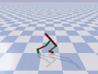
Voot Tangkaratt, Nontawat Charoenphakdee, Masashi Sugiyama

tions obtained by choosing demonstrations in D with           for our theoretical result in Section 3.1. Specifically,
gpxq ă 0, i.e., samples that are predicted to be drawn        recall that Theorem 1 relies on the equality in Eq. (14).
from ρN . This risk with pseudo-labeling enables us to        At the same time, the equality in Eq. (14) holds if the
empirically solve Eq. (9) in our setting. However, the        the following inequality holds:
trained classifier may perform poorly, mainly because
samples in P are labeled by the classifier itself. Specif-                     α ´ κpπqp1 ´ λq ą 0.                 (18)
ically, the classifier during training may predict the        This inequality depends on α, κpπq, and λ, where α
labels of demonstrations incorrectly, i.e., demonstra-        is unknown, κpπq depends on the policy, and λ is the
tions drawn from ρE pxq are incorrectly predicted to be       hyper-parameter. However, we cannot choose nor eval-
drawn from ρN pxq. This may degrade the performance           uate κpπq since we do not directly optimize κpπq during
of the classifier, because using incorrectly-labeled data     policy training. Thus, we need to choose an appropri-
can reinforce the classifier to be over-confident in its      ate value of λ so that the inequality in Eq. (18) al-
incorrect prediction (Kingma et al., 2014).                   ways holds. Recall that we assumed 0.5 ă α ă 1 in
To remedy the over-confidence of the classifier, we pro-      Section 2.3. Under this assumption, the inequality in
pose co-pseudo-labeling, which combines the ideas of          Eq. (18) holds regardless of the true value of α when
pseudo-labeling and co-training (Blum and Mitchell,           κpπqp1´λq ď 0.5. Since the value of κpπq increases to 1
1998). Specifically, we train two classifiers denoted by      as the policy improves by training (see Assumption 1),
g1 and g2 by minimizing the following empirical risks:        the appropriate value of λ is 0.5 ď λ ă 1.
                                                              However, a large value of λ may not be preferable
R             p D r`sym pg1 pxqqs ` λ E
p 1 pg1 q “ 1 E                       p P r`sym p´g1 pxqqs
            2 1                     2 1                       in practice since it increases the influence of pseudo-
              1´λp                                            labels on the risks (i.e., the second term in Eqs. (16)
           `        EB r`sym p´g1 pxqqs ,             (16)    and (17)). These pseudo-labels should not have larger
                2
                                                              influence than real labels (i.e., the third term in
p 2 pg2 q “ 1 E
R             p D r`sym pg2 pxqqs ` λ E
                                      p P r`sym p´g2 pxqqs    Eqs. (16) and (17)). For this reason, we decided to
            2 2                     2 2
              1´λp                                            use λ “ 0.5, which is the smallest value of λ that
           `        EB r`sym p´g2 pxqqs ,             (17)    ensures the inequality in Eq. (18) to be always held
                2
                                                              during training. Nonetheless, we note that while RIL-
where D1 and D2 are disjoint subsets of D. Pseudo-            Co with λ “ 0.5 already yields good performance in
labeled dataset P1 is obtained by choosing demonstra-         the following experiments, the performance may still
tions from D2 with g2 pxq ă 0, and pseudo-labeled             be improved by fine-tuning λ using e.g., grid-search.
dataset P2 is obtained by choosing demonstrations
from D1 with g1 pxq ă 0. With these risks, we re-             Remarks. Choosing λ “ 0 corresponds to omitting
duce the influence of over-confident classifiers because      co-pseudo-labeling, and doing so reduces RIL-Co to
g1 is trained using samples pseudo-labeled by g2 and          variants of GAIL which are not robust. Concretely,
vice-versa (Han et al., 2018). We call our proposed           the risk optimization problem of RIL-Co with λ “ 0
method Robust IL with Co-pseudo-labeling (RIL-Co).            is maxπ ming Rpg; ρ1 , ρπ , `sym q. By using the logistic
                                                              loss: `pzq “ logp1 ` expp´zqq, instead of a symmetric
We implement RIL-Co by using a stochastic gradient            loss, we obtain the following risk:
method to optimize the empirical risk where we al-
ternately optimize the classifiers and policy. Recall            2Rpg; ρ1 , ρπ , `q “ Eρ1 rlogp1 ` expp´gpxqqqs
from Eq. (9) that we aim to maximize Rpg; ρ1 , ρλπ , `sym q                        ` Eρπ rlogp1 ` exppgpxqqqs,      (19)
w.r.t. π. After ignoring terms that are constant
w.r.t. π, solving this maximization is equivalent to          which is the negative of GAIL’s objective in Eq. (4)3 .
maximizing Eρπ r`sym p´gpxqqs w.r.t. π. This objective        Meanwhile, we may obtain other variants of GAIL by
is identical to the RL objective in Eq. (1) with a re-        using summetric losses such as the sigmoid loss and the
ward function rpxq “ `sym p´gpxqq. Therefore, we can          unhinged loss (van Rooyen et al., 2015). In particular,
train the policy in RIL-Co by simply using an existing        with the unhinged loss: `pzq “ 1 ´ z, the risk becomes
RL method, e.g., the trust-region policy gradient (Wu         the negative of Wasserstein GAIL’s objective with an
et al., 2017). We summarize the procedure of RIL-Co           additive constant (Li et al., 2017; Xiao et al., 2019):
in Algorithm 1. Sourcecode of our implementation is                                                            1
available at https://github.com/voot-t/ril_co.                  2Rpg; ρ1 , ρπ , `q “ Eρ1 r´gpxqs ` Eρπ rgpxqs ` .   (20)
                                                                                                               2
                                                              However, even when `pzq is symmetric, we conjecture
3.3   Choice of Hyper-parameter
                                                              that such variants of GAIL are not robust, because
We propose to use λ “ 0.5 for RIL-Co, because it                3
                                                                  Here, ρ1 replaces ρE . The sign flips since RIL-Co and
makes the equality in Eq. (14) holds which is essential       GAIL solve max-min and min-max problems, respectively.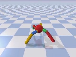
Robust Imitation Learning from Noisy Demonstrations

Algorithm 1 RIL-Co: Robust Imitation Learning with Co-pseudo-labeling
 1:    Input: Demonstration dataset D, initial policy π, and initial classifiers g1 and g2 .
 2:    Set hyper-parameter λ “ 0.5 (see Section 3.3) and batch-sizes (B “ U “ V “ 640 and K “ 128).
 3:    Split D into two disjoint datasets D1 and D2 .
 4:    while Not converge do
 5:      while |B| ă B with batch size B do
 6:         Use π to collect and include transition samples into B
 7:      Co-pseudo-labeling:
 8:         Sample txu uUu“1 from D2 , and choose K samples with g2 pxu q ă 0 in an ascending order as P1 .
 9:         Sample txv uVv“1 from D1 , and choose K samples with g1 pxv q ă 0 in an ascending order as P2 .
10:      Train classifiers:
11:         Train g1 by performing gradient descent to minimize the empirical risk Rp1 pg1 q using D1 , P1 and B.
12:         Train g2 by performing gradient descent to minimize the empirical risk Rp2 pg2 q using D2 , P2 and B.
13:      Train policy:
14:         Train the policy by an RL method with transition samples in B and rewards rpxq “ `sym p´g1 pxqq.

                                                                               3
Table 1: Examples of losses and their symmetric property, i.e.,
whether `pzq ` `p´zq “ c. We denote normalized counterparts                    2
of non-symmetric losses by (N). The AP loss in Eq. (21) is a
linear combination of the normalized logistic and sigmoid losses.              1

                                                                       ℓ(z)
      Loss name                   `pzq               Symmetric                 0
                                                                                     Logistic
      Logistic              logp1 ` expp´zqq             7                           Hinge
                                                                              −1
                                                                                     Sigmoid
      Hinge                   maxp1 ´ z, 0q              7                           Unhinged
                                                                              −2
                                                                                     Normalized logistic
      Sigmoid                1{p1 ` exppzqq              3                           Normalized hinge
                                                                              −3
      Unhinged                    1´z                    3                      −3   −2     −1       0     1   2    3
                                                                                                     z
                           logp1 ` expp´zqq
      Logistic (N)                                       3
                      ΣkPt´1,1u logp1 ` expp´zkqq                    Figure 1: The value of losses in Table 1. Non-
                             maxp1 ´ z, 0q                           symmetric losses, i.e., the logistic and hinge
      Hinge (N)                                          3
                       ΣkPt´1,1u maxp1 ´ zk, 0q                      losses, become symmetric after normalization.

λ “ 0 does not make the inequality in Eq. (18) holds         retical result in Section 3.1. In addition, any loss can
when κpπq ą 0.5.                                             be made symmetric by using normalization (Ma et al.,
                                                             2020). Therefore, the requirement of symmetric losses
3.4      Choice of Symmetric Loss                            is not a severe limitation. Table 1 and Figure 1 show
                                                             examples of non-symmetric and symmetric losses.
In our implementation of RIL-Co, we use the active-
passive loss (AP loss) (Ma et al., 2020) defined as          4      EXPERIMENTS
                          0.5 ˆ logp1 ` expp´zqq
       `AP pzq “                                             We evaluate the robustness of RIL-Co on continuous-
                   logp1 ` expp´zqq ` logp1 ` exppzqq        control benchmarks simulated by PyBullet simulator
                         0.5                                 (HalfCheetah, Hopper, Walker2d, and Ant) (Coumans
                  `              ,                    (21)
                     1 ` exppzq                              and Bai, 2019). These tasks are equipped with the true
                                                             reward functions that we use for the evaluation pur-
which satisfies `AP pzq ` `AP p´zq “ 1. This loss is a
                                                             pose. The learning is conducted using the true states
linear combination of two symmetric losses: the nor-
                                                             (e.g., joint positions) and not the visual observations.
malized logistic loss (the first term) and the sigmoid
                                                             We report the mean and standard error of the perfor-
loss (the second term). It was shown that this loss
                                                             mance (cumulative true rewards) over 5 trials.
suffers less from the issue of under-fitting when com-
pared to each of the normalized logistic loss or the         We compare RIL-Co with the AP loss against
sigmoid loss (Ma et al., 2020). However, we empha-           the following baselines: BC (Pomerleau, 1988),
size that any symmetric loss can be used to learn the        FAIRL (Ghasemipour et al., 2020), VILD (Tangkaratt
expert policy with RIL-Co, as indicated by our theo-         et al., 2020), and three variants of GAIL where each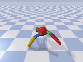
Voot Tangkaratt, Nontawat Charoenphakdee, Masashi Sugiyama
RIL-Co (AP) GAIL (logistic) GAIL (unhinged) GAIL (AP) FAIRL VILD BC
1e3 HalfCheetah 1e3 Hopper 1e3 Walker2D 1e3 Ant
2.5 3
Cumulative rewards
Cumulative rewards
Cumulative rewards
Cumulative rewards
2 2.0
2.0
1.5 1.5 2
1
1.0 1.0
1
0 0.5
0.5
0.0 0
0.0 0.1 0.2 0.3 0.4 0.0 0.1 0.2 0.3 0.4 0.0 0.1 0.2 0.3 0.4 0.0 0.1 0.2 0.3 0.4
Noise rate Noise rate Noise rate Noise rate
Figure 2: Final performance in continuous-control benchmarks with different noise rates. Vertical axes denote
cumulative rewards obtained during the last 1000 training iterations. Shaded regions denote standard errors
computed over 5 runs. RIL-Co performs well even when the noise rate increases. Meanwhile, the performance
of other methods significantly degrades as the noise rate increases.
1e3 HalfCheetah 1e3 Hopper 1e3 Walker2D 1e3 Ant
2.5 3.0
2
Cumulative rewards
2.0
Cumulative rewards
Cumulative rewards
Cumulative rewards
2.0 2.5
1 1.5 1.5 2.0
1.0 1.0 1.5
0
1.0
0.5 0.5 0.5
1
0.0 0.0 0.0
0.0 0.5 1.0 1.5 2.0 0.0 0.5 1.0 1.5 2.0 0.0 0.5 1.0 1.5 2.0 0.0 0.5 1.0 1.5 2.0
Transition samples 1e7 Transition samples 1e7 Transition samples 1e7 Transition samples 1e7
Figure 3: Performance against the number of transition samples in continuous-control benchmarks with noise
rate δ “ 0.4. RIL-Co achieves better performances and uses less transition samples compared to other methods.
variant uses different losses: logistic, unhinged, and numbers of transition samples. Then, we use the best
AP. As discussed in the remarks of Section 3.3, GAIL performing policy snapshot (in terms of cumulative re-
with the logistic loss denotes the original GAIL that wards) to collect 10000 expert state-action samples,
performs density matching with the Jensen-Shannon and use the other 5 policy snapshots to collect a to-
divergence, GAIL with the unhinged loss denotes a tal of 10000 non-expert state-action samples. Lastly,
variant of GAIL that performs density matching with we generate datasets with different noise rates by mix-
the Wasserstein distance, and GAIL with the AP loss ing expert and non-expert state-action samples, where
corresponds to RIL-Co without co-pseudo-labeling. noise rate δ P t0, 0.1, 0.2, 0.3, 0.4u approximately de-
termines the number of randomly chosen non-expert
All methods use policy networks with 2 hidden-layers
state-action samples. Specifically, a dataset consisting
of 64 hyperbolic tangent units. We use similar net-
of 10000 expert samples corresponds to a dataset with
works with 100 hyperbolic tangent units for classifiers
δ “ 0 (i.e., no noise), whereas a dataset consisting of
in RIL-Co and discriminators in other methods. The
10000 expert samples and 7500 randomly chosen non-
policy networks are trained by the trust region policy
expert samples corresponds to a dataset with δ “ 0.4
gradient (Wu et al., 2017) from a public implementa-
approximately4 . We note that the value of δ approxi-
tion (Kostrikov, 2018). The classifiers and discrimi-
mately equals to the value of 1 ´ α in Eq. (6).
nators are trained by Adam (Kingma and Ba, 2015)
with the gradient penalty regularizer with the regular- Figure 2 shows the final performance achieved by each
ization parameter of 10 (Gulrajani et al., 2017). The method. We can see that RIL-Co outperforms com-
total number of transition samples collected by the parison methods and achieves the best performance in
learning policy is 20 million. More details of experi- high noise scenarios where δ P t0.2, 0.3, 0.4u. Mean-
mental setting can be found in Appendix B. while, in low noise scenarios where δ P t0.0, 0.1u, RIL-
Co performs comparable to the best performing meth-
4.1 Evaluation on Noisy Datasets with ods such as GAIL with the logistic and AP losses.
Different Noise Rates Overall, the results show that RIL-Co achieves good
In this experiment, we evaluate RIL-Co on noisy performance in the presence of noises, while the other
datasets generated with different noise rates. To ob- methods fail to learn and their performance degrades
tain datasets, we firstly train policies by RL with the as the noise rate increases.
true reward functions. Next, we choose 6 policy snap- 4
The true noise rates of these datasets are as follows:
shots where each snapshot is trained using different δ̃ P t0, 1000{11000, 2500{12500, 5000{15000, 7500{17500u.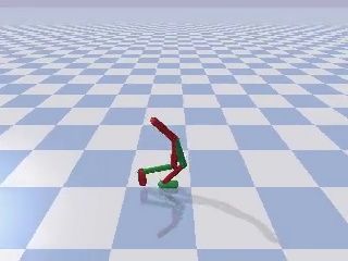
Robust Imitation Learning from Noisy Demonstrations
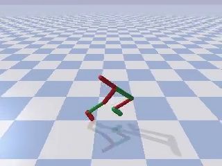
Figure 4: Visualization of the first 100 time steps of trajectories obtained by RIL-Co from datasets with noise
rate δ “ 0.4. Time step increases from the leftmost figure (t “ 0q to the rightmost figure (t “ 100q. RIL-Co
agents successfully solve these tasks. The obtained trajectories also closely resemble expert demonstrations.
In contrast, density matching methods, namely FAIRL forming GAIL) and gradually increasing the value to
and GAIL with the logistic and unhinged losses, do λ “ 0.5 as learning progresses.
not perform well. This is as expected, because these
On the other hand, VILD performs poorly with noisy
methods would learn a policy that is a mixture of the
datasets even with a small noise rate of δ “ 0.1. We
expert and non-expert policies and would not perform
conjecture that this is because VILD could not accu-
well. Also notice that GAIL with the unhinged loss
rately estimate the noise distributions due to the vio-
performs very poorly on the Walker2D and Ant tasks
lation of its Gaussian assumption. Specifically, VILD
even with noiseless demonstrations where δ “ 0. This
assumes that noisy demonstrations are generated by
is an intriguing result given that the unhinged loss is
adding Gaussian noise to actions drawn from the ex-
also symmetric similarly to the AP loss. We conjecture
pert policy, and that expert demonstrations consist
that the poor performance is due to the unbounded-
of low-variance actions. However, noisy demonstra-
ness from below of the unhinged loss (see Figure 1).
tions in this experiment are generated by using policy
This unboundedness may lead to a poorly behaved
snapshots without adding any noise. In this case, non-
classifier that outputs values with very large magni-
expert demonstrations may consist of low-variance ac-
tudes, as suggested by Charoenphakdee et al. (2019).
tions (e.g., non-expert policy may yield a constant ac-
With such a classifier, we expect that GAIL with the
tion). Due to this, VILD cannot accurately estimate
unhinged loss would require a strong regularization to
the noise distributions and performs poorly. Mean-
perform well, especially for complex control tasks.
while, behavior cloning (BC) does not perform well.
In addition, we can see that RIL-Co is more robust This is because BC assumes that demonstrations are
when compared to GAIL with the AP loss. This result generated by experts. It also suffers from the issue of
supports our theorem which indicates that a symmet- compounding error which worsens the performance.
ric loss alone is insufficient for robustness. Interest-
Next, Figure 3 shows the performance against the
ingly, with expert demonstrations (i.e., δ “ 0), GAIL
number of transition samples collected by the learn-
tends to outperform RIL-Co. This is perhaps because
ing policy for δ “ 0.4. RIL-Co achieves better per-
co-pseudo-labeling introduces additional biases. This
formances and uses less transition samples when com-
could be avoided by initially using λ “ 0 (i.e., per-
pared to other methods. This result indicates that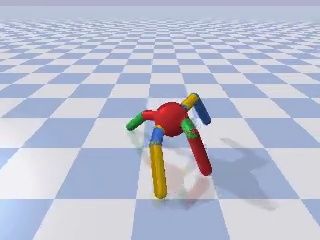
Voot Tangkaratt, Nontawat Charoenphakdee, Masashi Sugiyama
RIL-Co (AP) RIL-Co (logistic) RIL-P (AP) RIL-P (logistic)
HalfCheetah Hopper Walker2D Ant
2.6 1e3 1e3 1e3
3.5
1e3
2.5
Cumulative rewards
Cumulative rewards
Cumulative rewards
Cumulative rewards
2.4 2.2 3.0
2.0
2.2 2.0 2.5
1.5
2.0 1.8 2.0
1.0
1.8 1.6 1.5
0.5
0.0 0.1 0.2 0.3 0.4 0.0 0.1 0.2 0.3 0.4 0.0 0.1 0.2 0.3 0.4 0.0 0.1 0.2 0.3 0.4
Noise rate Noise rate Noise rate Noise rate
Figure 5: Final performance of variants of RIL-Co in the ablation study. RIL-Co with the AP loss performs the
best. This shows that using a symmetric loss and co-pseudo-labeling together is important for robustness.
RIL-CO is data efficient. Results for different noise 1e3 Ant
rates can be found in Appendix C, and they show a 2.5
similar tendency.
2.0
Cumulative rewards
Lastly, Figure 4 depicts visualization of trajectories
obtained by the policy of RIL-Co. Indeed, RIL-Co 1.5
agents successfully solve the tasks. The trajectories RIL-Co (AP) GAIL (AP)
also closely resemble expert demonstrations shown in 1.0 GAIL (logistic) FAIRL
GAIL (unhinged) VILD
Appendix B. This qualitative result further verifies
that RIL-Co successfully learns the expert policy. 0.5
0.0 0.0 0.5 1.0 1.5 2.01e7
4.2 Ablation Study
Transition samples
In this section, we conduct ablation study by eval- Figure 6: Performance with a Gaussian noise dataset.
uating different variants of RIL-Co. Specifically, we RIL-Co performs better than others except VILD.
evaluate RIL-Co with the logistic loss to investigate
the importance of symmetric loss. In addition, to
investigate the importance of co-pseudo-labeling, we Gaussian assumption of VILD is correct in this setting
also evaluate Robust IL with Pseudo-labeling (RIL-P) but incorrect in the previous setting. Still, RIL-Co
which uses naive pseudo-labeling in Eq. (15) instead of achieves a performance comparable to that of VILD
co-pseudo-labeling. Experiments are conducted using with 20 million samples, even though RIL-Co relies on
the same datasets in the previous section. a milder data generation assumption (see Section 2.3).
Meanwhile, the other methods do not perform as well
The result in Figure 5 shows that RIL-Co with the as RIL-Co and VILD.
AP loss outperforms the variants. This result further
indicates that using a symmetric loss and co-pseudo- Overall, the empirical results in our experiments indi-
labeling together is important for robustness. cate that RIL-Co is more robust against noisy demon-
strations when compared to existing methods.
4.3 Evaluation on Gaussian Noise Dataset
5 CONCLUSIONS
Next, we evaluate RIL-Co with the AP loss in the
Ant task with a noisy dataset generated by Gaussian We presented a new method for IL from noisy demon-
noise. Specifically, we use a dataset with 10000 expert strations. We proved that robust IL can be achieved
and 7500 non-expert state-action samples, where non- by optimizing a classification risk with a symmetric
expert samples are obtained by adding Gaussian noise loss, and we proposed RIL-Co which optimizes the risk
to action samples drawn from the expert policy. This by using co-pseudo-labeling. We showed through ex-
dataset is generated according to the main assumption periments that RIL-Co is more robust against noisy
of VILD (Tangkaratt et al., 2020), and we expect VILD demonstrations when compared to existing methods.
to perform well in this experiment.
In this paper, we utilized co-pseudo-labeling to ap-
Figure 6 depicts the performance against the number proximate data from non-expert densities. However,
of transition samples. It can be seen that VILD per- data from non-expert densities may be readily avail-
forms much better in this setting compared to the pre- able (Grollman and Billard, 2011). Utilizing such data
vious setting in Figure 2. This is as expected, since the for robust IL is an interesting future direction.
Robust Imitation Learning from Noisy Demonstrations

Acknowledgement                                             with extremely noisy labels. In Advances in Neural
                                                            Information Processing Systems.
We thank the reviewers for their useful comments. NC      Hastie, T., Tibshirani, R., and Friedman, J. (2001).
was supported by MEXT scholarship and Google PhD            The Elements of Statistical Learning. Springer New
Fellowship program. MS was supported by KAKENHI             York Inc.
17H00757.
                                                          Ho, J. and Ermon, S. (2016). Generative adversarial
                                                            imitation learning. In Advances in Neural Informa-
References
                                                            tion Processing Systems.
Angluin, D. and Laird, P. (1988). Learning from noisy     Kingma, D. P. and Ba, J. (2015). Adam: A method for
 examples. Machine Learning.                                stochastic optimization. In International Conference
Blum, A. and Mitchell, T. (1998). Combining labeled         on Learning Representations.
  and unlabeled data with co-training. In Interna-        Kingma, D. P., Mohamed, S., Jimenez Rezende, D.,
  tional Conference on Computational Learning The-          and Welling, M. (2014). Semi-supervised learning
  ory.                                                      with deep generative models. In Advances in Neural
Brodersen, K. H., Ong, C. S., Stephan, K. E., and           Information Processing Systems.
  Buhmann, J. M. (2010). The balanced accuracy and        Kostrikov, I. (2018). Pytorch implementations of re-
  its posterior distribution. In International Confer-     inforcement learning algorithms. https://github.
  ence on Pattern Recognition.                             com/ikostrikov/pytorch-a2c-ppo-acktr-gail.
Brown, D., Coleman, R., Srinivasan, R., and Niekum,       Li, Y., Song, J., and Ermon, S. (2017). Infogail: Inter-
  S. (2020). Safe imitation learning via fast bayesian      pretable imitation learning from visual demonstra-
  reward inference from preferences. In International       tions. In Advances in Neural Information Processing
  Conference on Machine Learning.                           Systems.
Brown, D. S., Goo, W., Nagarajan, P., and Niekum,         Lu, N., Niu, G., Menon, A. K., and Sugiyama, M.
  S. (2019). Extrapolating beyond suboptimal demon-         (2019). On the minimal supervision for training any
  strations via inverse reinforcement learning from ob-     binary classifier from only unlabeled data. In Inter-
  servations. In International Conference on Machine        national Conference on Learning Representations.
  Learning.
                                                          Ma, X., Huang, H., Wang, Y., Romano, S., Erfani,
Chapelle, O., Schlkopf, B., and Zien, A. (2010). Semi-     S., and Bailey, J. (2020). Normalized loss functions
  Supervised Learning. The MIT Press, 1st edition.         for deep learning with noisy labels. In International
Charoenphakdee, N., Lee, J., and Sugiyama, M.              Conference on Machine Learning.
  (2019). On symmetric losses for learning from cor-      Mandlekar, A., Zhu, Y., Garg, A., Booher, J., Spero,
  rupted labels. In International Conference on Ma-        M., Tung, A., Gao, J., Emmons, J., Gupta, A., Or-
  chine Learning.                                          bay, E., Savarese, S., and Fei-Fei, L. (2018). ROBO-
Coumans, E. and Bai, Y. (2016–2019). Pybullet, a           TURK: A crowdsourcing platform for robotic skill
  python module for physics simulation for games,          learning through imitation. In Conference on Robot
  robotics and machine learning. http://pybullet.          Learning.
  org.                                                    Menon, A., Narasimhan, H., Agarwal, S., and Chawla,
Ghasemipour, S. K. S., Zemel, R., and Gu, S. (2020).       S. (2013). On the statistical consistency of al-
 A divergence minimization perspective on imitation        gorithms for binary classification under class im-
 learning methods. In Proceedings of the Conference        balance. In International Conference on Machine
 on Robot Learning.                                        Learning.
Grollman, D. H. and Billard, A. (2011). Donut as I        Natarajan, N., Dhillon, I. S., Ravikumar, P. K., and
  do: Learning from failed demonstrations. In IEEE          Tewari, A. (2013). Learning with noisy labels. In Ad-
  International Conference on Robotics and Automa-          vances in Neural Information Processing Systems.
  tion, ICRA, pages 3804–3809.                            Ng, A. Y. and Russell, S. J. (2000). Algorithms for in-
Gulrajani, I., Ahmed, F., Arjovsky, M., Dumoulin, V.,       verse reinforcement learning. In International Con-
 and Courville, A. C. (2017). Improved training of          ference on Machine Learning.
 wasserstein gans. In Advances in Neural Information      Pomerleau, D. (1988). ALVINN: an autonomous land
 Processing Systems.                                        vehicle in a neural network. In Advances in Neural
Han, B., Yao, Q., Yu, X., Niu, G., Xu, M., Hu,              Information Processing Systems.
  W., Tsang, I. W., and Sugiyama, M. (2018). Co-          Puterman, M. L. (1994). Markov Decision Processes:
  teaching: Robust training of deep neural networks         Discrete Stochastic Dynamic Programming.
Voot Tangkaratt, Nontawat Charoenphakdee, Masashi Sugiyama Schaal, S. (1999). Is imitation learning the route to humanoid robots? Trends in Cognitive Sciences. Silver, D., Schrittwieser, J., Simonyan, K., Antonoglou, I., Huang, A., Guez, A., Hubert, T., Baker, L., Lai, M., Bolton, A., Chen, Y., Lillicrap, T., Hui, F., Sifre, L., van den Driessche, G., Graepel, T., and Hassabis, D. (2017). Mastering the game of Go without human knowledge. Nature. Sun, W., Vemula, A., Boots, B., and Bagnell, D. (2019). Provably efficient imitation learning from observation alone. In International Conference on Machine Learning. Syed, U., Bowling, M. H., and Schapire, R. E. (2008). Apprenticeship learning using linear programming. In International Conference on Machine Learning. Tangkaratt, V., Han, B., Khan, M. E., and Sugiyama, M. (2020). Variational imitation learning with diverse-quality demonstrations. In International Conference on Machine Learning. van Rooyen, B., Menon, A., and Williamson, R. C. (2015). Learning with symmetric label noise: The importance of being unhinged. In Advances in Neu- ral Information Processing Systems 28. Wu, Y., Charoenphakdee, N., Bao, H., Tangkaratt, V., and Sugiyama, M. (2019). Imitation learning from imperfect demonstration. In International Confer- ence on Machine Learning. Wu, Y., Mansimov, E., Grosse, R. B., Liao, S., and Ba, J. (2017). Scalable trust-region method for deep reinforcement learning using kronecker-factored ap- proximation. In Advances in Neural Information Processing Systems. Xiao, H., Herman, M., Wagner, J., Ziesche, S., Ete- sami, J., and Linh, T. H. (2019). Wasserstein ad- versarial imitation learning. CoRR, abs/1906.08113. Ziebart, B. D., Bagnell, J. A., and Dey, A. K. (2010). Modeling interaction via the principle of maximum causal entropy. In International Conference on Ma- chine Learning.
Robust Imitation Learning from Noisy Demonstrations

A     PROOFS
A.1   Proof of Lemma 1

We firstly restate the main assumption of our theoretical result:
Assumption 1 (Mixture state-action density). The state-action density of the learning policy π is a mixture of
the state-action densities of the expert and non-expert policies with a mixing coefficient 0 ď κpπq ď 1:
                                        ρπ pxq “ κpπqρE pxq ` p1 ´ κpπqqρN pxq,                                   (22)
where ρπ pxq, ρE pxq, and ρN pxq are the state-action densities of the learning policy, the expert policy, and the
non-expert policy, respectively.

Under this assumption and the assumption that ρ1 ps, aq “ αρE ps, aq ` p1 ´ αqρN ps, aq, we obtain Lemma 1.
Lemma 1. Letting `sym p¨q be a symmetric loss that satisfies `sym pgpxqq ` `sym p´gpxqq “ c, @x P X and a
constant c P R, the following equality holds.
                                                                                     1 ´ α ` κpπqp1 ´ λq
                 Rpg; ρ1 , ρλπ , `sym q “ pα ´ κpπqp1 ´ λqqRpg; ρE , ρN , `sym q `                       c.       (23)
                                                                                              2

Proof. Firstly, we define κ̃pπ, λq “ κpπqp1 ´ λq and δ ` pxq “ `pgpxqq ` `p´gpxqq. Then, we substitute ρ1 pxq :“
αρE pxq ` p1 ´ αqρN pxq and ρπ pxq “ κpπqρE pxq ` p1 ´ κpπqqρN pxq into the risk Rpg; ρ1 , ρλπ , `q.
 2Rpg; ρ1 , ρλπ , `q “ Eρ1 r`pgpxqqs ` Eρλπ r`p´gpxqqs
                 “ Eρ1 r`pgpxqqs ` p1 ´ λqEρπ r`p´gpxqqs ` λEρN r`p´gpxqqs
                 “ αEρE r`pgpxqqs ` p1 ´ αqEρN r`pgpxqqs
                   ` pκpπqp1 ´ λqqEρE r`p´gpxqqs ` p1 ´ κpπqqp1 ´ λqEρN r`p´gpxqqs ` λEρN r`p´gpxqqs
                 “ αEρE r`pgpxqqs ` p1 ´ αqEρN r`pgpxqqs ` κ̃pπ, λqEρE r`p´gpxqqs ` p1 ´ κ̃pπ, λqqEρN r`p´gpxqqs
                                                    “                 ‰
                 “ αEρE r`pgpxqqs ` p1 ´ αqEρN δ ` pxq ´ `p´gpxqq
                                 “                  ‰
                  ` κ̃pπ, λqEρE δ ` pxq ´ `pgpxqq ` p1 ´ κ̃pπ, λqqEρN r`p´gpxqqs
                                                    “     ‰
                 “ αEρE r`pgpxqqs ` p1 ´ αqEρN δ ` pxq ´ EρN r`p´gpxqqs ` αEρN r`p´gpxqqs
                                 “     ‰
                  ` κ̃pπ, λqEρE δ ` pxq ´ κ̃pπ, λqEρE r`pgpxqqs ` EρN r`p´gpxqqs ´ κ̃pπ, λqEρN r`p´gpxqqs
                                                                                   “      ‰          “       ‰
                 “ pα ´ κ̃pπ, λqq pEρE r`pgpxqqs ` EρN r`p´gpxqqsq ` p1 ´ αqEρN δ ` pxq ` κ̃pπ, λqEρE δ ` pxq
                                                                “       ‰             “       ‰
                 “ 2pα ´ κ̃pπ, λqqRpg; ρE , ρN , `q ` p1 ´ αqEρN δ ` pxq ` κ̃pπ, λqEρE δ ` pxq .               (24)

For symmetric loss, we have δ `sym pxq “ `sym pgpxqq ` `sym p´gpxqq “ c for a constant c P R. With this, we can
express the left hand-side of Eq. (23) as follows:
                                                               p1 ´ αq     “         ‰ κpπqp1 ´ λq       “           ‰
 Rpg; ρ1 , ρλπ , `sym q “ pα ´ κpπqp1 ´ λqqRpg; ρE , ρN , `sym q `     EρN δ `sym pxq `               EρE δ `sym pxq
                                                                  2                           2
                                                               p1 ´ αq            κpπqp1 ´ λq
                    “ pα ´ κpπqp1 ´ λqqRpg; ρE , ρN , `sym q `         EρN rcs `              EρE rcs
                                                                  2                    2
                                                               1 ´ α ` κpπqp1 ´ λq
                    “ pα ´ κpπqp1 ´ λqqRpg; ρE , ρN , `sym q `                      c.                             (25)
                                                                        2
This equality concludes the proof of Lemma 1. Note that this proof follows Charoenphakdee et al. (2019).

A.2   Proof of Theorem 1

Lemma 1 indicates that, when α ´ κpπqp1 ´ λq ą 0, we have
                                             g ‹ “ argmin Rpg; ρ1 , ρλπ , `sym q
                                                         g

                                                “ argmin Rpg; ρE , ρN , `sym q.                                   (26)
                                                         g

With this, we obtain Theorem 1 which we restate and prove below.
Voot Tangkaratt, Nontawat Charoenphakdee, Masashi Sugiyama
Theorem 1. Given the optimal classifier g ‹ in Eq. (26), the solution of maxπ Rpg ‹ ; ρ1 , ρλπ , `sym q is equivalent to
the expert policy.
Proof. By using the definitions of the risk and ρλπ pxq, Rpg ‹ ; ρ1 , ρλπ , `sym q can be expressed as
1 λ 1´λ
Rpg ‹ ; ρ1 , ρλπ , `sym q “ Eρ1 r`sym pg ‹ pxqqs ` EρN r`sym p´g ‹ pxqqs ` Eρπ r`sym p´g ‹ pxqqs . (27)
2 2 2
Since the first and second terms are constant w.r.t. π, the solution of maxπ Rpg ‹ ; ρ1 , ρλπ , `sym q is equivalent to the
solution of maxπ Eρπ r`sym p´g ‹ pxqqs, where we omit the positive constant factor p1 ´ λq{2. Under Assumption 1
which assumes ρπ pxq “ κpπqρE pxq ` p1 ´ κpπqqρN pxq , we can further express the objective function as
Eρπ r`sym p´g ‹ pxqqs “ κpπqEρE r`sym p´g ‹ pxqqs ` p1 ´ κpπqqEρN r`sym p´g ‹ pxqqs
´ ¯
“ κpπq EρE r`sym p´g ‹ pxqqs ´ EρN r`sym p´g ‹ pxqqs ` EρN r`sym p´g ‹ pxqqs . (28)
The last term is a constant w.r.t. π and can be safely ignored. The right hand-side is maximized by increasing
κpπq to 1 when the inequality EρE r`sym p´g ‹ pxqqs ´ EρN r`sym p´g ‹ pxqqs ą 0 holds. Since g ‹ is also the optimal
classifier of Rpg; ρE , ρN , `sym q, the inequality EρE r`sym p´g ‹ pxqqs ´ EρN r`sym p´g ‹ pxqqs ą 0 holds. Specifically,
the expected loss of classifying expert data as non-expert: EρE r`sym p´g ‹ pxqqs, is larger to the expected loss
of classifying non-expert data as non-expert: EρN r`sym p´g ‹ pxqqs. Thus, the objective can only be maximized
by increasing κpπq to 1. Because κpπq “ 1 if and only if ρπ pxq “ ρE pxq, we conclude that the solution of
maxπ Rpg ‹ ; ρ1 , ρλπ , `sym q is equivalent to πE .
B DATASETS AND IMPLEMENTATION
We conduct experiments on continuous-control benchmarks simulated by PyBullet simulator (Coumans and Bai,
2019). We consider four locomotion tasks, namely HalfCheetah, Hopper, Walker2d, and Ant, where the goal
is to control the agent to move forward to the right. We use true states of the agents and do not use visual
observation. To obtain demonstration datasets, we collect expert and non-expert state-action samples by using
6 policy snapshots trained by the trust-region policy gradient method (ACKTR) (Wu et al., 2017), where each
snapshot is obtained using different training samples. The cumulative rewards achieved by the six snapshots
are given in Table 2, where snapshot #1 is used as the expert policy. Visualization of trajectories obtained by
the expert policy in these tasks is provided in Figure 7. Sourcecode of our datasets and implementation for
reproducing the results is publicly available at https://github.com/voot-t/ril_co.
All methods use policy networks with 2 hidden-layers of 64 hyperbolic tangent units. We use similar networks
with 100 hyperbolic tangent units for classifiers in RIL-Co and discriminators in other methods. The policy
networks are trained by ACKTR, where we use a public implementation (Kostrikov, 2018). In each iteration,
the policy collects a total of B “ 640 transition samples using 32 parallel agents, and we use these transition
samples as the dataset B in Algorithm 1. Throughout the learning process, the total number of transition samples
collected by the learning policy is 20 million. For training the classifier and discriminator, we use Adam (Kingma
and Ba, 2015) with learning rate 10´3 and the gradient penalty regularizer with the regularization parameter of
10 (Gulrajani et al., 2017). The mini-batch size for classifier/discriminator training is 128.
For co-pseudo-labeling in Algorithm 1 of RIL-Co, we initialize by splitting the demonstration dataset D into
two disjoint subset D1 and D2 . In each training iteration, we draw batch samples U “ txu uU u“1 „ D2 and
V “ txv uVv“1 „ D1 from the split datasets with U “ V “ 640. To obtain pseudo-labeled datasets P1 for training
classifier g1 , we firstly compute the classification scores g2 pxu q using samples in U. Then, we choose K “ 128
samples with the least negative values of g2 pxu q in an ascending order as P1 . We choose samples in this way to
incorporate a heuristic that prioritizes choosing negative samples which are predicted with high confidence to be
negative by the classifiers, i.e., these samples are far away from the decision boundary. Without this heuristic,
obtaining good approximated samples requires using a large batch size which is computationally expensive. The
procedure to obtain P2 is similar, but we use V instead of U and g1 pxv q instead of g2 pxu ). The implementation
of RIL-P variants in our ablation study is similar, except that we have only one neural networks and we do not
split the dataset into disjoint subsets.
For VILD, we the log-sigmoid reward variant and perform important sampling based on the estimated noise, as
described by Tangkaratt et al. (2020). For behavior clonig (BC), we use a deterministic policy neural networkRobust Imitation Learning from Noisy Demonstrations
Table 2: Cumulative rewards achieved by six policy snapshots used for generating demonstrations. Snapshot 1 is
used as the expert policy. Ant (Gaussian) denotes a scenario in the experiment with the Gaussian noise dataset
in Section 4.3, where Gaussian noise with different variance is added to expert actions.
Task Snapshot #1 Snapshot #2 Snapshot #3 Snapshot #4 Snapshot #5 Snapshot #6
HalfCheetah 2500 1300 1000 700 -1100 -1000
Hopper 2300 1100 1000 900 600 0
Walker2D 2700 800 600 700 100 0
Ant 3500 1400 1000 700 400 0
Ant (Gaussian) 3500 1500 1000 800 500 400
Figure 7: Visualization of the first 100 time steps of expert demonstrations. Time step increases from the leftmost
figure (t “ 0q to the rightmost figure (t “ 100q. Videos are provided with the sourcecode.
and train it by minimizing the mean-squared-error with Adam and learning rate 10´3 . We do not apply a
regularization technique for BC. For the other methods, we follow the original implementation as close as possible,
where we make sure that these methods perform well overall on datasets without noise.
C ADDITIONAL RESULTS
Here, we present learning curves obtained by each method in the experiments. Figure 8 depicts learning curves
(performance against the number of transition samples collected by the learning policy) for the results in Sec-
tion 4.1. Since BC does not use the learning policy to collect transition samples, the horizontal axes for BC
denote the number of training iterations. It can be seen that RIL-Co achieves better performances and uses less
transition samples compared to other methods in the high-noise scenarios where δ P t0.2, 0.3, 0.4u. Meanwhile
in the low-noise scenarios, all methods except GAIL with the unhinged loss and VILD perform comparable to
each other in terms of the performance and sample efficiency.
Figure 9 shows learning curves of the ablation study in Section 4.2. RIL-Co with the AP loss clearly outperforms
the comparison methods in terms of both sample efficiency and final performance. The final performance in
Figures 2 and 5 are obtained by averaging the performance in the last 1000 iterations of the learning curves.You can also read