NOTTINGHAM CORE HMA HOUSING MARKET NEEDS ASSESSMENT UPDATE 2009 - Rushcliffe B.Line Housing Information Ltd
←
→
Page content transcription
If your browser does not render page correctly, please read the page content below
NOTTINGHAM CORE HMA

HOUSING MARKET NEEDS
    ASSESSMENT

      UPDATE 2009

         Rushcliffe

  B.Line Housing Information Ltd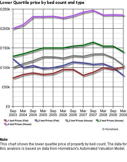
Table of Contents

1)     Introduction ............................................................................................................................... 1
            Figure 1:1 Average annual build rate targets as set out in the East Midlands RSS8 2006
            and 2009 ............................................................................................................................... 1
            Figure 1:2 Bramley affordability model – summary ............................................................... 2
2)     Key Figures and Comparisons.................................................................................................. 5
            Figure 2:1 Key Variable settings for LA and submarket model outputs ................................. 5
            Figure 2:2 Local Authority Level Needs Estimates ................................................................ 6
     2.2.      Comparisons with results from 2006.................................................................................. 7
       2.2.1.         Lower Quartile Prices ................................................................................................. 7
            Figure 2:3 Change in lower quartile price 2006/2009 (LA Level)........................................... 7
       2.2.2.         Affordability................................................................................................................. 7
            Figure 2:4 Percentage of emerging households unable to afford market purchase .............. 7
            Figure 2:5 Split of main income bands .................................................................................. 7
       2.2.3.         Gross Need, Supply and Net Need ............................................................................ 8
            Figure 2:6 Need and Supply.................................................................................................. 8
3)     House Prices ............................................................................................................................ 9
            Figure 3:1 Property Sales Count (June 2007 to March 2009) ............................................... 9
            Figure 3:2 Change in count of sales, June 2007 to March 2009 ......................................... 10
            Figure 3:3 Count of sales – month on month comparison (June 2007 – March 2009) ........ 10
            Figure 3:4 Average House Prices (Comparison) Nottingham Core LAs.............................. 11
       3.1.2.         Lower Quartile Price Fluctuations by Bed Count and Property Type........................ 12
            Figure 3:5 Lower Quartile price by bed count and type - Rushcliffe Local Authority ........... 12
            Figure 3:6 Comparison of lower quartile prices by property type and size – all Local
            Authorities ........................................................................................................................... 12
            Figure 3:7 Local authority level number of sales by property type and size ........................ 13
4)     Supply..................................................................................................................................... 13
            Figure 4:1 Local authority level annual supply .................................................................... 13
5)     Households in need ................................................................................................................ 14
     5.1.      Backlog Need .................................................................................................................. 14
            Figure 5:1 HSSA data (2005 – 2008) .................................................................................. 14
            Figure 5:2 Comparison of average and trend figures from HSSA data (2009 projection).... 14
            Figure 5:3 Waiting List Growth (HSSA data), 2009 value takes trend figure ....................... 15
     5.2.      Emerging Households ..................................................................................................... 15
Figure 5:4 Emerging Households by local authority ............................................................ 15
5.3. Owner Occupier Need ..................................................................................................... 16
Figure 5:5 Estimated levels of owner occupation by local authority .................................... 16
5.4. Migrations ........................................................................................................................ 17
Figure 5:6 Migration statistics by local authority.................................................................. 17
6) Key Variables.......................................................................................................................... 18
Figure 6:1 Scenarios changing 3 key variables and results ................................................ 18
6.2. Rent and Purchase Price Differentials ............................................................................. 19
Figure 6:2 Impact of Private Rental Sector monthly cost variations on affordability
percentages by LA .............................................................................................................. 20
Figure 6:3 Comparison of need figures - lower quartile purchase and rent (Key Variables
set as above)....................................................................................................................... 20
6.3. Intermediate Housing....................................................................................................... 20
Figure 6:4 Intermediate Housing Scope – Emerging Households Only............................... 21
Figure 6:5 Intermediate Housing Scope – All households including backlog need ............. 21
7) Results and Submarket Outputs ............................................................................................. 22
Figure 7:1 Key variable settings for results and submarket outputs .................................... 22
7.2. Deriving submarket level needs figures ........................................................................... 22
Figure 7:2 Discussion of sources and methodology for model outputs ............................... 22
Figure 7:3 Model outputs at Local Authority level - Rushcliffe............................................. 26
7.2.2. Submarket Outputs - Rushcliffe................................................................................ 27
Figure 7:4 Rushcliffe Submarkets ....................................................................................... 27
Figure 7:5 Key outputs by submarket (Rushcliffe)............................................................... 28
7.3. Submarket Output Comparisons by Local Authority, 2006 and 2009 outputs.................. 29
Figure 7:6 Submarket Level Output comparisons, Rushcliffe.............................................. 29
8) Key Conclusions and Recommendations ............................................................................... 30
8.1.1. Rushcliffe.................................................................................................................. 30
8.1.2. Area Summary – Nottingham Core Housing Market Area ........................................ 301) Introduction
1.1.1.a. The UK housing market has undergone a turbulent and well publicised period of
change since the Nottingham Core HMA 2006/7 was carried out. Although house prices have
reduced to some extent across the board, in many areas they remain well above long term
incomes multipliers and now combine with the additional barrier of increasingly stringent
mortgage application criteria, as well as demands for larger deposits (many of the best
mortgage deals require a deposit of 15 to 25%). The delay in a market adjustment may be
exacerbated by a lingering determination among vendors to achieve peak values for their
homes, as well as a need to reach a certain price to repay mortgages (particularly if a
purchase was made during the 2004 – 2007 boom). The onset of economic recession has
been accompanied by increased unemployment, though housing need as a result of this more
recent development may not yet have filtered through to the data sources used for this
analysis.
1.1.1.b. All evidence indicates that the need for affordable housing has not disappeared and
imbalances continue to be evident across housing markets. Recent observations include
continued growth in the number of repossessions; an increase in competition across the
private rental sector; owner occupiers unable to sell turning increasingly to renting their homes
(and moving into the sector themselves) to cover costs; and a slowdown in the rate of new
developments.
1.1.1.c. The review of the East Midlands Regional Plan (RSS8) 2009 contains significant
increases to the build targets across the Nottingham Core Housing Market Area. This may be
a reflection both of the continued pressure on the public sector to provide new housing as well
as a build up effect, because of the slowdown in the number of new developments. A
continued recession is likely to reduce the possibility of meeting these increased targets, as
developers and land owners wait for a market recovery.
Figure 1:1 Average annual build rate targets as set out in the East Midlands RSS8 2006 and 2009
Local Authority Annual Build Rate Target 2006 Annual Build Rate Target 2009
Broxtowe 270 340
Erewash 290 360
Gedling 310 400
Nottingham 945 1000
Rushcliffe 555 750
1.1.1.d. Increased build rate targets are coupled with a requirement to ensure the economic
viability of affordable housing provision on any new development sites (following the Blythe
Valley case1), which is also delaying the provision of new housing as sites are examined.
1.1.1.e. The reliability of the outputs contained in this update can only be as good as the data
itself. There are often discrepancies between the level of detail at which data is available, the
timescale or categorisation by which it is gathered, as well as inevitable gaps in data relating to
factors like migration or the private rental sector.
1
See http://www.bailii.org/ew/cases/EWCA/Civ/2008/861.html
11.1.1.f. Several housing needs spreadsheet models were developed as part of the 2006/7
Nottingham core Strategic Housing Market Assessment, based on the ‘Bramley’ model. This
captures the main components of housing need of:-
• New emerging households that cannot afford market housing, with the ability to afford
estimated by comparing entry level house prices or private sector rents to incomes
• Backlog need based on local authority housing registers
• A factor for owner occupiers falling into need
• An element for need from migrations
1.1.1.g. This is then compared to the supply of affordable lets and sales from local authorities
and housing associations.
1.1.1.h. The model can be summarised as:-
Figure 1:2 Bramley affordability model – summary
The basic model for estimating affordable housing need is as follows:-
Net Need (units per year) =
Gross Household Formation x % aged under 35 unable to buy (adjusted for wealth)
+ proportion (33%) x net migration (household equiv) x %• House price and house price change patterns
• Short distance moves
• Urban morphology which subdivides the built up area , such as major roads, railway lines,
parks, commercial and industrial areas, open space, etc
• Local knowledge – this more subtle, implicit awareness of differences is often found to be
the best indicator of the real urban structure 3
1.1.1.l. For this update the submarket model has been developed further, also using ‘larger’
submarket areas which have proved to be useful in policy development for Nottingham City
Council. The updated model also includes several more detailed and accurate data sources,
such as using actual housing registers records and lettings data, rather than proxy estimates.
But models at these more detailed spatial scales cannot yet, if ever, capture the flows and
migrations between submarket areas, which are extremely complex and variable.
1.1.1.m. This means that even if some submarkets show little or no need in themselves,
supply within them may meet needs arising from elsewhere, so there may be good reasons for
providing additional affordable housing in them, such as available land or lower prices.
However it does also mean that local authorities should be particularly cautious about creating
a local over supply of affordable housing and concentrating deprivation, or increasing the level
of ‘churning’ within an area resulting in increased unpopularity and poor reputation.
1.1.1.n. They remain simply data driven models which must rely on the quality and coverage
of the data inputs to them, and which cannot capture the full complexity of needs in a dynamic,
shifting and inefficient housing market. The data and models provide part of the evidence base
and a decision support system, but policy judgments and interventions should also take into
account and balance more up to date qualitative local knowledge, experience and perceptions.
1.1.1.o. The methods used in the 2009 model reiterate those followed in the 2006 HMA
report.4 However, there are some differences between the datasets which are likely to have an
impact on the resulting outputs. These factors are listed below:
1. Emerging Households: In the 2006/7 submarket model emerging households were derived
using Census data, rolled forward to estimate how many people would have reached the 18-
35 age group and formed households. Though this method has been used again in this
model for the smaller submarkets, where possible figures are derived from ONS population
projections by lower super output area, 2007 which should include additional growth from
migration and other factors.
2. The income element of the affordability calculations at submarket level in 2006/7 was
derived using the ASHECASS model, which attributes earnings from the Annual Survey of
Hours and Earnings (given at local authority level by occupation) to socio-economic groups
based on the Census. Incomes in the 2009 model are based on CACI incomes data by
ward (for LA level data, 2009), or by postcode (2006) for submarket level data.
3. For the 2009 model CACI income bands most sensitive to entry level price changes (i.e.
£15K -£30K) were split into four to increase the responsiveness of the model.
4. The 2009 model includes a basic search of rental costs by submarket which adds an
additional affordability factor which may be discounted to give ‘urgent’ need.
5. Backlog need in the 2009 model is derived from actual detailed waiting list data where
available. Where this is not available, HSSA totals are allocated across submarkets
according to the corresponding proportion of households in the private rented sector in each
3
https://www.researchgate.net/publication/23772013_Forecasting_Housing_Prices_under_Different_Submarket_Assumptions
4
See http://www.blinehousing.info/NottCore_HMA/SHMA_report_sections/Housing_need.PDF
3submarket based on the 2001 Census. In 2006 backlog need was estimated by using the
Private Rented Sector adjusted for affordability using ASHECASS. As a proxy this matched
fairly well with HSSA totals in 2006, but significant growth in waiting lists more recently and
the growing time difference makes the proxy less robust. feasible.
6. The owner occupier need factor has been increased from 0.234% or 1 in 427 to 0.345% or 1
in 290, based on an increase in the number of repossessions. The figure used is derived
from statistics published by the Council of Mortgage Lenders in 2008.
7. An additional element has been added to allow for the increasingly important role of the
private rented sector in serving those who are somewhere between purchase and social
rent, by choice or otherwise. The model allows the effect of different rent levels on overall
affordability to be examined, and provides an indication of the number of households likely
to fall into each group (can’t rent/can’t buy).
42) Key Figures and Comparisons
2.1.1.a. The outputs produced by the model are based on the following:
• House Prices from March 2008 to March 2009
• CACI Incomes data, 2009 (LA level only, submarket analysis uses 2006 incomes data)
• Emerging households calculations are based on, depending on the level of detail:
o Chelmer Model projections by household type/Local Authority
o ONS population projections by Lower Super Output Area (for larger submarkets)
o Census 2001 population by age group by Output Area, rolled forwards to 2008 (for
some smaller submarkets)
• Private rental sector rents are based on a basic web search of prices as advertised on
www.rightmove.co.uk, rent levels by local authority as published on
www.dataspring.org.uk, and cross-tenure affordability data provided by the Hometrack
Housing Intelligence System, www.hometrack.co.uk).
• Backlog need data is based on HSSA returns and waiting list data where available.
Where housing waiting list data has not been available, the HSSA total is allocated
across submarkets to match the proportions of private rent in each submarket as at the
Census 2001, based on the assumption that need will arise mainly from this tenure.
Problems with deriving backlog need in this way are discussed later.
• Supply is based on local authority lettings data where available, and CORE data. Totals
are compared with HSSA returns to assess accuracy.
Key Variables are set as follows, unless stated otherwise:
Figure 2:1 Key Variable settings for LA and submarket model outputs
KEY VARIABLES Inputs in white cells
House Price Fluctuation 0%
Mortgage Multiplier 3.5
Size of Deposit 10%
Policy Period (years) 7.5
Proportion unable to access mortgage 51%
Owner Occupier Need Factor 0.345%
Equity Share in Intermediate Housing
Products 40%
% with resources from other sources 0%
Lower quartile private rent level (Rent Service =
1; Submarket Average = 2; Housing Intelligence
=3 1
5Figure 2:2 Local Authority Level Needs Estimates
Total
Emerging Emerging Lower % can't Emerging Private % can't
Households Households Quartile Income afford Households Rent afford
LA (10 years) (annual) Price required purchase can't afford LQP rent
Broxtowe 8,852 885 £120,000 £30,857 52% 460 £394 17%
Erewash 7,853 785 £95,000 £24,429 40% 314 £360 13%
Gedling 7,403 740 £100,000 £25,714 39% 289 £416 19%
Nottingham 29,956 2,996 £82,500 £21,214 39% 1,168 £373 18%
Rushcliffe 8,213 821 £139,995 £35,999 50% 411 £412 14%
Annual
Owner Need Backlog backlog
Owner Occupier from Need (Policy GROSS
Occupiers Need migration (HSSA) Period) NEED
Broxtowe 21,250 73 80 2,344 313 92
Erewash 23,099 80 8 3,627 484 86
Gedling 23,570 81 19 3,275 437 26
Nottingham 37,498 129 124 17,083 2,278 3,699
Rushcliffe 20,789 72 46 1,452 194 723
Annual Proportion able to Number
Supply afford but unable unable to Total unable to afford +
(Net of NET to access access unable to access
transfers) NEED mortgage mortgage mortgage
Broxtowe 481 445 24% 212 672
Erewash 529 357 31% 243 557
Gedling 430 396 31% 229 518
Nottingham 3,410 289 31% 929 2,097
Rushcliffe 361 362 26% 213 624
62.2. Comparisons with results from 2006
2.2.1. Lower Quartile Prices
Figure 2:3 Change in lower quartile price 2006/2009 (LA Level)
Lower Quartile Price Lower Quartile Price
LA 2005-06 2008-09
Broxtowe £103,000 £120,000
Erewash £93,125 £95,000
Gedling £105,000 £100,000
Nottingham £85,000 £82,500
Rushcliffe £142,000 £139,995
2.2.1.b. Given the level of speculation in the media, on an aggregated basis across the
housing market area there is surprisingly little change in lower quartile house prices across
each local authority. Broxtowe alone shows a significant change, though house prices have
gone up, not down. This corroborates the notion that many of those unable to purchase
property in 2006 are now little closer to affording their own home.
2.2.2. Affordability
2.2.2.c. The following table compares the percentage of emerging households unable to
afford market purchase, deducting 10% who may have access to financial resources from
elsewhere (for example parental help), as applied in the 2006 study. The method of splitting
the most highly populated income bands (see figure 2.5 below) means the later model picks up
more people below the lower quartile threshold.
Figure 2:4 Percentage of emerging households unable to afford market purchase
2006 unable to afford (minus 2009 unable to afford
10% resources from (minus 10% resources
LA elsewhere) from elsewhere)
Broxtowe 30% 47%
Erewash 32% 36%
Gedling 29% 35%
Nottingham 38% 35%
Rushcliffe 42% 45%
2.2.2.d. As the income range for lower quartile housing so often lies within the most common
incomes, the bands containing the largest number of people have been split evenly into 4 as
follows:
Figure 2:5 Split of main income bands
Income Band Split 1 Split 2 Split 3 Split 4
£15,000 - £20,000 £16,250 £17,500 £18,750 £20,000
£20,000 - £25,000 £21,250 £22,500 £23,750 £25,000
£25,000 - £30,000 £26,250 £27,500 £28,750 £30,000
2.2.2.e. Although splitting in this way will not be an altogether accurate reflection of reality, it
will help to give an improved indication of the volatility of this factor. In the most populated
income bands, a relatively small change in house prices can move large numbers of
households in or out of the need calculation.
72.2.3. Gross Need, Supply and Net Need
Figure 2:6 Need and Supply
LA Waiting Waiting Gross Gross Supply Supply Net Need Net Need
List 2006 List 2009 Need Need 2006 2009 2006 2009
2006 2009
Broxtowe 2,508 2,344 733 882 465 481 168 401
Erewash 1,633 3,627 560 855 238 529 199 326
Gedling 2,700 3,275 675 796 450 430 153 366
Nottingham 14,270 17,083 3,484 3,580 3,190 3,410 192 170
Rushcliffe 1,442 1,452 701 681 298 361 236 320
2.2.3.f. The main area of change over the period has been the growth in size of the housing
registers across Erewash, Gedling and Nottingham. Though the waiting list has decreased in
Broxtowe, house prices have gone up bringing more emerging households into need. Overall,
although supply does show growth, it is not enough to reverse the trend of growing need for
more affordable housing.
83) House Prices
3.1.1.a. House prices have been under constant scrutiny, first because they seemed to be
rising inextricably beyond the reach of almost all average incomes, then since the market has
begun to correct at the expense of the economy.
3.1.1.b. The Hometrack Housing Intelligence System is used below to give an overview of
prices across the 4 local authority areas.
3.1.1.c. The overall frequency of sales has fallen drastically across all areas since 2007,
towards the end of the housing boom. Both linear and month to month comparisons show a
steady decline in the number of purchases, although the seasonal nature of the market is still
evident. This fall in the number of sales reflects, among other things, continued affordability
problems, barriers to access for potential purchasers, consumers waiting for further price drops
before they enter the market, and fewer properties remaining on the market while prices are
falling. In addition, continued economic recession and widespread instability in the
employment sector are likely to undermine the confidence of potential buyers.
Figure 3:1 Property Sales Count (June 2007 to March 2009)
Date Rushcliffe Nottingham Broxtowe Gedling Erewash
Jun-07 698 1,516 627 626 624
Jul-07 729 1,582 672 679 692
Aug-07 790 1,732 712 802 759
Sep-07 676 1,727 667 742 728
Oct-07 638 1,696 604 709 681
Nov-07 545 1,517 623 614 595
Dec-07 512 1,334 568 600 543
Jan-08 427 1,158 504 532 472
Feb-08 361 1,019 365 458 432
Mar-08 316 942 327 375 408
Apr-08 345 961 318 354 433
May-08 357 917 320 352 433
Jun-08 355 863 336 360 445
Jul-08 348 804 329 358 393
Aug-08 338 723 319 319 339
Sep-08 324 673 276 315 279
Oct-08 304 605 281 288 289
Nov-08 263 565 243 249 271
Dec-08 236 524 252 240 256
Jan-09 192 440 191 175 192
Feb-09 147 320 148 137 127
Mar-09 84 168 63 46 60
9Figure 3:2 Change in count of sales, June 2007 to March 2009
Increase/Decrease in Sales by LA (June 2007 = 0)
200
Rushcliffe
Nottingham
150 Broxtowe
Gedling
100 Erewash
50
0
Jun- Jul- Aug- Sep- Oct- Nov- Dec- Jan- Feb- Mar- Apr- May- Jun- Jul- Aug- Sep- Oct- Nov- Dec- Jan- Feb- Mar-
07 07 07 07 07 07 07 08 08 08 08 08 08 08 08 08 08 08 08 09 09 09
-50
-100
-150
-200
-250
Figure 3:3 Count of sales – month on month comparison (June 2007 – March 2009)
Count of Sales - comparing month/month
2000
1800
1600
1400
1200
1000
800
600
400
200
0
Rushcliffe Nottingham Broxtowe Gedling Erewash
Jun-07 Jun-08 Jul-07 Jul-08 Aug-07 Aug-08 Sep-07 Sep-08 Oct-07 Oct-08
Nov-07 Nov-08 Dec-07 Dec-08 Jan-08 Jan-09 Feb-08 Feb-09 Mar-08 Mar-09
Source: Housing Intelligence System. Hometrack (www.hometrack.co.uk)
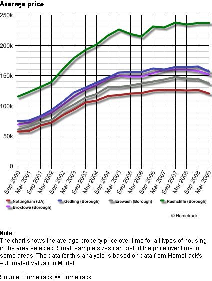
103.1.1.d. The trend of average price over time for the whole study area shows decreasing
prices have had little impact on the steep inflation shown across all five local authorities since
2002.
Figure 3:4 Average House Prices (Comparison) Nottingham Core LAs
113.1.2. Lower Quartile Price Fluctuations by Bed Count and Property Type
Figure 3:5 Lower Quartile price by bed count and type - Rushcliffe Local Authority
3.1.2.e. Prices in Rushcliffe are the highest across the whole study area, for all property
types. The gaps between each property type (or each ‘rung’ on the property ladder) are more
comparatively stable than the other authorities. As prices for 2 bed flats and 2 and 3 bed
houses have all declined, 1 bed flat prices show an upturn over the last quarter, converging
with 2 bed houses. However, 1 bed flat prices generally seem more volatile than other
property types, so it is unsafe to make any judgement based on price movement during only
one quarter.
Figure 3:6 Comparison of lower quartile prices by property type and size – all Local Authorities
Compare Lower Quartile Prices by Property Type & Size
March 2009 Broxtowe Erewash Gedling Nottingham Rushcliffe
1 bed flat £55,000* £68,000* £52,200* £50,000 £101,000
2 bed flat £68,500 £73,000 £88,500 £75,000 £80,000
2 bed house £90,000 £83,500 £95,000 £71,000 £106,000
3 bed house £109,300 £105,000 £100,000 £80,000 £140,000
4 bed house £163,000 £152,000 £175,000 £105,000 £235,000
*Sep-08 price has been used where Mar-09 price is unavailable
Source: Hometrack Housing Intelligence System
123.1.2.f. There continues to be a clear hierarchy between prices in the city and prices in the
more suburban authorities. Rushcliffe clearly carries a premium which is probably attributable
to its more rural character. The hierarchy is least evident in relation to 2 bed flats, for which
prices are very similar and Gedling shows as the most expensive. In terms of frequency there
are far fewer sales of flats than houses, which is a clear reflection of market demand
(particularly since we know there is currently an abundant supply of flats available). Three bed
houses remain the most commonly purchased property in all local authorities.
Figure 3:7 Local authority level number of sales by property type and size
Property Count by property type and size
Sept 2008 Nottingham Broxtowe Gedling Erewash Rushcliffe
1 bed flat 68 9 10 9 10
2 bed flat 175 44 39 8 40
2 bed house 537 284 204 386 156
3 bed house 1,161 683 510 716 433
4 bed house 265 172 154 143 270
Mar-09 count is unavailable
4) Supply
4.1.1.a. Supply figures at LA level are based on CORE RSL lettings and HSSA data. The
CORE entries for LA stock are included in the model for reference but are not used at this level
(to avoid duplication with HSSA data). However, where LAs currently holding social housing
stock do not participate in CORE this poses a problem with disaggregating the data to
submarket level.
4.1.1.b. Across all local authorities the total yearly lettings recorded in the 2008 HSSA data
were less than those recorded in 2007, indicating a downward trend. Erewash and Rushcliffe
have transferred all their stock to RSLs, so their HSSA entry is zero. In this example, the trend
has been used to estimate annual supply from local authorities, rather than the average (which
is higher and does not reflect the apparent reduction in annual lets).
Figure 4:1 Local authority level annual supply
Result Total (select
Lettings Net Lettings Net of from Average appropriate results to
of Transfers Transfers CORE Annual HA combine for annual
LA 2007 2008 Trend Average data Lettings supply)
2007 2008 2009 2009
Broxtowe 401 375 349 388 175 132 481
Erewash 0 0 0 0 0 529 529
Gedling 313 299 285 306 184 145 430
Nottingham 2,780 2,696 2,612 2,738 0 798 3,410
Rushcliffe 0 0 0 0 60 301 361
135) Households in need
5.1. Backlog Need
5.1.1.a. The numbers on the waiting list are taken from HSSA returns, and move differently
for each local authority. The trend has been used rather than the average – this decision must
be judgment based and which figure is appropriate may vary for each authority. Apart from
Broxtowe and Gedling, all authorities show an increase in numbers on their waiting lists,
though the numbers in Rushcliffe have remained fairly stable. The figure used in the needs
calculation will need to take account of internal knowledge of waiting list changes. In all cases,
the number of applicants for housing far outstrips supply.
Figure 5:1 HSSA data (2005 – 2008)
Section C: Housing waiting list and choice-based lettings
Households on the housing waiting list at 1st April
1a. Total households on the housing waiting list at 1st April Trend
LA 2005 2006 2007 2008 2009
Broxtowe 2,502 2,508 2,293 2,448 2,344
Erewash 0 1,633 2,482 2,386 3,627
Gedling 4,849 5,218 3,251 4,074 3,275
Nottingham 11,329 13,201 14,159 15,668 17,083
Rushcliffe 1,534 1,442 1,535 1,451 1,452
Figure 5:2 Comparison of average and trend figures from HSSA data (2009 projection)
LA Average annual waiting list Trend
Broxtowe 2,438 2,344
Erewash 1,625 3,627
Gedling 4,348 3,275
Nottingham 13,589 17,083
Rushcliffe 1,491 1,452
14Figure 5:3 Waiting List Growth (HSSA data), 2009 value takes trend figure
Waiting List Growth
18000
2005
2006
16000 2007
2008
2009
14000
12000
10000
8000
6000
4000
2000
0
Broxtowe Erewash Gedling Nottingham Rushcliffe
5.2. Emerging Households
5.2.1.b. A proportion of emerging households will be unable to afford accommodation at
open market cost. Data for emerging households is taken from the DCLG/Chelmer Household
Projections, 2004. These projections are particularly useful in needs analysis as they give a
breakdown by age and household type, as well as providing an estimate of average household
size. This allows the emerging households (given to be between 18 and 35) to be isolated
fairly effectively (in theory). Results are shown below. The period considered is 10 years,
based on the projections for 2011 and 2021. The model calculates how many households over
that time will move through the emerging households age group, and apportions them
annually. Numbers are similar for all authorities except Nottingham, which obviously has a
greater number of new households as a large city.
Figure 5:4 Emerging Households by local authority
Emerging households over 10 Annual emerging
LA years households
Broxtowe 8,852 885
Erewash 7,853 785
Gedling 7,403 740
Nottingham 29,956 2,996
Rushcliffe 8,213 821
155.3. Owner Occupier Need
5.3.1.c. The model derives owner occupation levels by taking the number of owner occupiers
(who live in their home, with a mortgage, including shared ownership) at the 2001 Census as a
baseline, then increasing this by 1% per year (x 1.08), based on the addition of new stock, to
give an estimate of the number of owner occupiers in the housing market today. This level of
growth could be argued up or down, because:
• During the beginning of the boom, more people were entering the property market than
before with easier access to capital and a huge number of incentives.
• Towards the end of the boom, fewer people could afford to enter the property market
because of unprecedented house price inflation.
5.3.1.d. A report by Savills Research (February 2009)5, based on the Survey of English
Housing suggests a fairly steep decline in owner occupation, which is being replaced by
private renting. Would-be buyers are kept in the private rental sector while they are priced out
of the purchase market. This situation is upheld by the continued (though lately more limited)
availability of buy-to-let mortgages. However, many transactions during the boom were
remortgages or purchases by existing owner occupiers using capital from their own home,
which could contribute significantly to need if these households are unable to service their
debt.
Figure 5:5 Estimated levels of owner occupation by local authority
Owner Proportion Increase to
Occupied with of 2009 (+1%
LA All Households mortgage households per year)
Ashfield 46,601 18,870 40% 20,380
Broxtowe 45,422 19,676 43% 21,250
Erewash 46,219 21,388 46% 23,099
Gedling 47,546 21,824 46% 23,570
Nottingham 116,070 34,720 30% 37,498
Rushcliffe 43,648 19,249 44% 20,789
5.3.1.e. According to the Council of Mortgage Lenders, 1 in 290 mortgages were
repossessed during 2008. They have predicted a rise in this proportion during 2009, though
because of technical issues with data compatibility the final number of repossessions predicted
will be revised downwards6. The 1 in 290 (or 0.345%) figure has been used to assess owner
occupier need in the latest model, though this figure can be revised up or down if new figures
emerge. This is an increase from the figure originally used in the previous adaptation of the
Bramley model (0.234%, or 1 in 427), and reflects the increased risk to owner occupiers in
today’s market.
5
“The decline of owner-occupation”, Savills Research (February 2009) last accessed 29 May 2009,
http://www.grantmanagement.co.uk/media/resources/Savills%20Feb%2009.pdf
6
See CML Press Release, 15 May 2009 (last accessed 29 May 2009),
http://www.cml.org.uk/cml/media/press/2262
165.4. Migrations
5.4.1.f. Migration statistics are difficult to incorporate, as they tend to be slightly behind other
population data given the transient nature of the group, but may be already accounted for to
some extent in emerging households and population growth projections. As the model uses
2004 projections in deriving emerging households, more recent net migration may add to the
total number of households potentially in need.
5.4.1.g. The migration figures used in the model are therefore based on ‘ONS population
projections: Natural change and migration summaries for local authorities and higher
administrative areas (2006)’, and take the ‘all migration net’ figure for each local authority. This
is then divided by the average household size (using the 2011 projection figure) to give an
estimate of the number of migrant households. Based on the Bramley model, it is assumed
that around a third of migrant households who are in need will apply for affordable housing.
5.4.1.h. The accuracy of these figures is questionable in relation to housing need, as it is
very difficult to know how many migrants remain in the area long term, how many actually
apply for housing, or whether there is a significant difference in household size. The
assumption that their socio-economic status, incomes and affordability criteria will be the same
as other residents is also debatable.
Figure 5:6 Migration statistics by local authority
ONS Net
Migration
LA ONS Net Migration (2008) ONS Net Migration (2009) (2010)
Broxtowe 1,100 1,000 1,000
Erewash 100 100 200
Gedling 300 300 400
Nottingham 2,400 2,000 1,700
Rushcliffe 600 600 700
%
% likely
Ave. hsehld Number of unable to
size (from migrant Annual to afford apply Need
Migrations over 3 years 2011 households migrant market for from in-
LA (people) projections) over 3 years households housing AH migrants
Broxtowe 3,100 2.221 1396 465 52% 33% 80
Erewash 400 2.22 180 60 40% 33% 8
Gedling 1,000 2.21 452 151 39% 33% 19
Nottingham 6,100 2.107 2895 965 39% 33% 124
Rushcliffe 1,900 2.291 829 276 50% 33% 46
176) Key Variables
6.1.1.a. The model allows key variables to be altered to assess the potential impact on need.
The significance of each variable can be considerable. Fluctuations in house price, the policy
period over which backlog need is addressed, and the number of households with resources
from other sources have the largest impact on the resulting need figure. A figure for the
proportion of households able to afford but unable to access mortgage capital7 is given in the
table below, and has a significant impact on the overall number of households who cannot
owner occupy, but is not applied to the needs figure as it is unlikely that those households
would apply for or want social housing. Four scenarios are given below.
Figure 6:1 Scenarios changing 3 key variables and results
Base Scenario Scenario Scenario
KEY VARIABLES scenario 1 2 3
House Price Fluctuation 0% -15% 0% 0%
Mortgage Multiplier 3.5 3.5 3.5 3.5
Size of Deposit 10% 10% 10% 10%
Policy Period 7.5 7.5 5 7.5
Proportion unable to access
mortgage 51% 51% 51% 51%
Owner Occupier Need Factor 0.345% 0.345% 0.345% 0.345%
Equity Share in Intermediate
Housing Products 40% 40% 40% 40%
% with resources from other
sources 10% 10% 10% 0%
Broxtowe Erewash Gedling Nottingham Rushcliffe
Net Need (Base Scenario) 561 342 405 419 411
Net Need (Scenario 1) 408 273 333 172 321
Net Need (Scenario 2) 717 583 623 1,558 507
Net Need (Scenario 3) 605 373 435 538 453
7
Based on Council of Mortgage Lenders statistic, 51% decline in the number of loans since January 2008
186.2. Rent and Purchase Price Differentials
6.2.1.b. The needs figures given throughout this report are based on affordability of lower
quartile house prices. However, there is a clear and relatively wide gap between social renting
and owner occupation which is filled frequently, and often effectively, by private renting.
Although private renting in Britain has historically been seen as a ‘stopgap’, temporary tenure,
it has been argued that the continued imbalance in housing markets and increasing separation
of the link between earnings and ownership have led to a shift in its role8.
6.2.1.c. As a result, the use of lower quartile house prices as a measure of affordability may
give an unrealistically high indication of the demand for social housing. In actuality, people
may be happy to remain in private renting for the longer term, rather than apply for social
housing after a period if unable to buy.
6.2.1.d. To attempt to account for this argument within the model, a secondary need figure
has been generated which deducts those households who can afford lower quartile private
rent9 from the total figure unable to afford lower quartile purchase. The remaining households
left in need are those that are more likely to more urgently require social housing, being unable
to afford anything else. A judgment is then required as to which figure most accurately reflects
the true picture, as not all people in private renting will be happy or suitably housed (though
this is true of all tenures). This also prompts an argument for further focus on the private
rented sector to ensure that those who do remain in the tenure long term are well treated and
protected.
6.2.1.e. Establishing a realistic lower quartile rental cost figure (for which the supply and
quality is an adequate substitute for the alternative of social housing) is difficult. Reported rent
levels vary, and variation can potentially make a large difference to the residual need figures.
In the example below, the monthly rent levels for each local authority have been derived using
data from Dataspring, which refers to the Rent Service. Because these rents are used to
calculate local housing allowance, they are more likely to be at the lower end of the market.
Using the Rent Service figure gives a much lower (and in some cases negative) result.
6.2.1.f. The model includes two other figures for private rental costs which may be applied to
assess the different impacts on residual need (those who cannot afford to rent or buy will be
the most urgent candidates for social housing). The two alternative figures are taken from an
average of submarket private rent levels (based on a search of www.rightmove.co.uk), and
cross-tenure affordability data provided by the Hometrack Housing Intelligence System
(www.hometrack.co.uk). The impact of changing private rental costs on the model is shown
below.
8
See “The Private Rented Sector: its contribution and potential”, Julie Rugg and David Rhodes, Centre for
Housing Policy, The University of York (2008), at
http://www.york.ac.uk/inst/chp/publications/PDF/prsreviewweb.pdf and
http://www.homesandcommunities.co.uk/private_rented_sector_initiative
9
Based on private rent levels by LA provided by dataspring (www.dataspring.org.uk). Submarket lower quartile
rents are based on a search of Rightmove for properties within the area, top of the first 25% of entries is selected.
Although not the most exact method, it gives a reasonably good indication of supply in the sector.
19Figure 6:2 Impact of Private Rental Sector monthly cost variations on affordability percentages by LA
% unable to afford based on
LA Rent Service Submarket Average Housing Intelligence System
Broxtowe 17% 23% 28%
Erewash 13% 24% 24%
Gedling 19% 16% 24%
Nottingham 18% 28% 36%
Rushcliffe 14% 17% 24%
Residual need figure (can't rent, can't buy) based on:
LA Rent Service Submarket Average Housing Intelligence System
Broxtowe 135 189 233
Erewash 145 231 231
Gedling 248 225 285
Nottingham -340 -40 200
Rushcliffe 66 91 148
Figure 6:3 Comparison of need figures - lower quartile purchase and rent (Key Variables set as above)
Lower Private Total can't NET NET
Quartile Income % can't Rent LQP % can't afford NEED NEED
LA Price required afford (monthly) afford PRS (Purchase) (PRS)
Broxtowe £120,000 £30,857 52% £394 17% 150 605 135
Erewash £95,000 £24,429 40% £360 13% 63 373 145
Gedling £100,000 £25,714 39% £416 19% 141 435 248
Nottingham £82,500 £21,214 39% £373 18% 330 538 -340
Rushcliffe £139,995 £35,999 50% £412 14% 115 453 66
6.2.1.g. In addition to the problem of establishing accurate lower quartile rental prices to use
in the model is the issue of supply within the private rental sector. Despite the appearance of
affordability in the private sector, the general upward trend of growth in local authority waiting
lists suggests the stock on offer is not adequate to meet demand. This may be due to a
combination of factors such as:
• Short supply of the property types and sizes that people want or need
• Difficulty raising deposits or acquiring references to access private rent
• Bad experiences or similar prompting people to apply for social housing where they may
otherwise have remained in private renting
• Low security of tenure (fear of unfair treatment, rent increases or eviction) creating an
impetus to apply for social housing (particularly in times of economic instability)
• Low supply for emerging households (much of the activity and movement within the
private rented sector occurs among those households already established in it).
6.3. Intermediate Housing
6.3.1.h. The model provides two calculations relating to intermediate housing based on the
latest available lower quartile prices. The two outputs are based on a variable equity stake (so
should be specific to individual sites) and detail:
201. The proportion of emerging households only able to afford intermediate housing at the
given equity stake
2. The proportion of all households unable to afford market housing able to afford
intermediate housing at the given equity stake
n.b. The second option makes the assumption that households on the housing register cannot
afford any form of tenure other than social housing. This is a broad assumption and is likely to
considerably underestimate the potential scope for intermediate housing products in terms of
affordability.
Below is an example of each output for intermediate housing scope.
Figure 6:4 Intermediate Housing Scope – Emerging Households Only
Proportion Total
able to unable to
No. afford but Number afford +
Proportion households unable to unable to unable to
unable to unable to access access access
Tenure/Product afford afford mortgage mortgage mortgage
Emerging
Hshlds
Only: Emerging
Number Hshlds
unable to Only: IH
afford scope (as
market % of
housing but affordable
able to housing
Purchase 52% 460 afford IH provided) 24% 212 672
Intermediate at
70% 34% 301 159 34.6% 34% 301 602
Intermediate at
50% 20% 177 283 61.5% 41% 363 540
Variable
proportion for
Intermediate
Housing
40% 12% 106 354 76.9%
Private Rent 29% 257
Figure 6:5 Intermediate Housing Scope – All households including backlog need
Proportion of Social Housing 54%
Proportion of Intermediate Housing 46%
At Equity Share of 40%
This social/intermediate split incorporates backlog need into the affordability calculation for intermediate
housing. It involves a policy decision to prioritise backlog need over future need.
6.3.1.i. The logic behind the calculation for the potential scope of intermediate housing is
that the lower the equity stake, the more households will be able to afford it. However, this
does not incorporate factors such as lower interest in lower equity stakes from potential
buyers.
6.3.1.j. Secondly, the intermediate housing calculation within the model assumes that new
build intermediate housing property values will not behave in the same way as resale
properties, and will retain a higher market value for longer (as with other new build properties).
Consequently, intermediate sale prices in the model do not respond to a drop in overall market
21prices. The result of this is that as house prices fall in the general market, the potential scope
for intermediate housing products diminishes (which should more accurately reflect reality).
7) Results and Submarket Outputs
7.1.1.a. Key Variables are set as follows:
Figure 7:1 Key variable settings for results and submarket outputs
KEY VARIABLES
House Price Fluctuation 0%
Mortgage Multiplier 3.5
Size of Deposit 10%
Policy Period 7.5
Proportion unable to access mortgage 51%
Owner Occupier Need Factor 0.345%
Equity Share in Intermediate Housing Products 40%
% with resources from other sources 0%
7.2. Deriving submarket level needs figures
7.2.1.b. Finding data which is detailed and recent enough to allow submarket modeling is
very difficult and involves many assumptions, proxy calculations and substitutions where the
ideal data is unavailable. The following table details the output requirements we want, the data
needed to provide them, and the substitutes or proxies used in the final model with
accompanying methods and potential inaccuracies. Whenever the model is updated this
‘shopping list’ should be referred to and the closest available dataset supplied wherever
possible to achieve a more accurate picture. Where submarkets cross administrative local
authority boundaries these are included within the model twice, under each local authority for
reference, and highlighted so users will be aware need for those submarkets will be duplicated.
Figure 7:2 Discussion of sources and methodology for model outputs
Output Data Required Data obtained Data used
Household size from
Chelmer Model (2011
Chelmer Model (LA Level) figure); Population
Household Projections; projections aggregated
ONS 2007 population to submarket. Census
projections by LSOA, counts rolled forward to
Number of new households Census data where today to estimate
requiring housing annually by submarkets do not fit LSOA emerging households
Emerging households submarket data. in smaller submarkets.
22Age groups in 2007 population projections are 16-29 and 30-44. The numbers in each
age group are disaggregated apportioning an equal number of people to each year of
the age group and reaggregated to include only the ages in question (i.e. 18-29 and
30-35). This figure is then divided by the average household size as taken from the
Chelmer projections. The household figure is then divided by 10, assuming new
households will emerge from this age group over 10 years. Census age groups who
will have reached the emerging households group since 2001 are selected and the
total divided by the average household size for those submarkets which do not contain
Method Applied an LSOA total.
Using a uniform average household size across all submarkets probably creates an
‘ecological fallacy’, assuming most households are the average size when in fact, most
are either larger or smaller, and there is almost certainly variation between submarkets.
Separating the age groups in the projections equally ignores the probability that there
are more people in one age group than another. The average household size in 2011
is subject to change, in fact some sources indicate that households are now growing
Potential Inaccuracies due to affordability problems.
House prices selected
by submarket and
lower quartile derived
Land Registry House Price (top of first 25%),
data, postcode level, Affordability (owner-
(Jan08-Feb09); CACI occupation) = count of
Incomes data by output area households unable to
(2006); Private rental lower afford LQP borrowing
quartile price derived using 3.5 x income;
Rightmove search (by Affordability (PRS) =
submarket where possible, count of households
Number of households or using sample postcode + unable to afford
unable to afford to buy/rent 1/4 mile), selecting top of LQRentalP paying 30%
Affordability by submarket lowest 25% of returns. of income.
Rank sales by submarket/price then derive lower quartile for each submarket. Assume
10% deposit and 3.5 times borrowing for purchase. Assume access to deposit for rent
and affordability at 30% of income. Total number of households in each income band
by submarket. Split most common income bands to allow for greater sensitivity in
affordability calculations (i.e. split households with income of £15,000 - £30,000). Total
number in each submarket unable to rent/buy at lower quartile price. Affordability
proportion is this number as a percentage of the total households in the submarket. (A
factor has been added to account for the number of households with resources from
Method Applied elsewhere, though this figure is also unknown locally).
The lower quartile price can be distorted by some very low end sales which may not
reflect market reality for most households and can provide an underestimation of
prices. Land registry data does not include bedroom counts, so lower quartiles can
only be derived by property type, not size. Ideally a lower quartile by property size
could tell us what kind of affordability levels there are by household type (i.e. singles,
couples, families, large families etc), however it is also difficult to access data on
household types and sizes more recent than the Census. We might assume that
emerging households (to which this factor will be applied) are naturally smaller and will
Potential Inaccuracies begin by purchasing or renting smaller (therefore cheaper) properties.
Migrations are not included
in the submarket
calculations as ONS
population estimates by
Number of migrants unable to LSOA (2007) have been
afford market used to estimate emerging
accommodation who are households, and should
In migrant households eligible and would apply for include a migration element
and affordability affordable housing in their totals n/a
Method Applied n/a
23Migration figures can vary greatly especially in periods of economic volatility. The
current economic downturn has reportedly seen many migrant workers leaving the
country, unable to find work or unsatisfied with the cost of living. A large exodus of
migrants can have a significant impact on the private rental sector in particular, for
which migrants have been a key market in certain areas. This could both increase
supply in the private sector, and raise issues with stock condition (as conditions of
overcrowding and poor quality stock have been argued to be more acceptable to
transient communities). There may have been a change in the level of migration since
the 2007 projections came out, although the overall impact of migration on needs
figures is small. However, if certain submarkets are more affected than others by
Potential Inaccuracies migrant movements, this may not be reflected.
Tenure aggregated to
submarket level and
Number of owner occupiers inflated based on
Owner occupier group (with a mortgage) by Tenure by output area, additional stock growth
size submarket Census 2001 (Table KS18) since 2001
The number of owner occupiers in each submarket at the 2001 Census is taken as a
baseline. The number with mortgages (including shared ownership) is extracted and
inflated by 1.08 (1% per year) to give an estimate of owner occupation levels today.
Method Applied The 1% represents the average additional stock growth.
Since the Census 2001 households have been getting older in most areas. This
suggests that many of the households with a mortgage in 2001 may now wholly own
their properties. In addition to this, there has been a steep drop in the number of first
time buyers entering the market. It is not possible to know the true levels of owner
occupation today. Some submarkets may have become hotspots for private renting
(particularly in student areas), leading to a decline in owner occupation, while others
may have had a boom in owner occupation because of a new scheme or development.
Potential Inaccuracies These variations at local level cannot be picked up by the model without local input.
The 1 in 290 figure
Number of owner occupiers (0.345%) is applied to
falling into housing need as a the projected number
result of arrears, eviction or National figure from CML (1 of owner occupiers in
Owner occupier need repossession by submarket in 290, 2008) each submarket.
The number of owner occupiers falling into housing need is quite a large unknown.
Due to growth in unemployment and a high number of households bearing high debt
levels it has been projected that there will be a rise in repossessions before the
economy starts to recover. However, moves by the Bank of England to keep rates low
and pressure on financial institutions to support financially troubled households may
have a downward impact on the number in this category. Deriving a figure for each
submarket is almost impossible without detailed information on repossessions at a
local level. It may be that repossessions are more common in certain areas, or for
Potential Inaccuracies certain property types or sizes.
For Nottingham City For Nottingham CC,
Council, waiting list data by Rushcliffe BC and
submarket (where Broxtowe BC, waiting
households live now); For list by submarket; for
Rushcliffe Borough Council, other councils proxy
waiting list data by postcode based on the Private
(where households live Rented Sector as at the
now); for Broxtowe Borough 2001 Census, which
Number of households on the Council, waiting list data by apportions the HSSA
waiting list by submarket sub-area (where households waiting list by
(ideally giving which wish to live); Gedling submarket according to
submarket they want to live Borough Council/Erewash the distribution of
in, rather than where they live Borough Council, no data private renting as at the
Backlog need now), excluding transfers available Census 2001.
24Where detailed waiting list data is provided, a count of backlog households by
submarket is derived and spread over the policy period. Where no data has been
provided a proxy has been used which allocates the total number of households on the
HSSA waiting list (based on 2009 trend projections) across each submarket
proportionately, based on the proportions in the private rented sector in each
submarket in 2001(based on the Census). The private rented sector is used as a
proxy, as it is assumed that this is a temporary tenure from which households will want
Method Applied to either buy or move into social housing.
Without genuine waiting list data we cannot be sure where need is emerging from, or
for. The private rented sector (PRS) is increasing less a temporary form of tenure for
many households, who do want to buy but do not want or need the option of social
housing. Government initiatives have encouraged the development of the PRS as a
more secure tenure, and some initial steps are being taken to improve the tenure and
make it more secure for households through greater support and regulation. There has
been very significant growth in the PRS over recent years, particularly through buy to
let mortgages and increased interest in property investment. The situation of
Nottingham as a university location also affects the distribution of the private rented
sector in a manner which may not accurately reflect the need for social housing based
on the proxy used in the model. However, because of the lack of available data as
discussed, the 2001 PRS distribution is the best proxy we have available to estimate
need at submarket level. Where waiting list data is used there are also discrepancies,
where totals do not match those given in the HSSA returns. There is also no way of
telling where people want to live as opposed to where they are living when they apply,
Potential Inaccuracies and the data collected in waiting lists varies.
For NCC and Broxtowe
BC, lettings by
submarket; for
Erewash and Gedling
BC CORE lettings by
submarket increased
CORE lettings data; proportionately to
Nottingham UA lettings by match HSSA totals
RSL and LA annual lettings postcode; Broxtowe BC lets where there is a
Supply by submarket by sub-area significant discrepancy.
Since not all local authorities participate fully in CORE there are some discrepancies
between the lettings count in the HSSA and in CORE (see tab CompareHSSA_CORE).
In the case of Erewash and Rushcliffe, all stock has been transferred to RSLs so
should all be accounted for in CORE. Nottingham UA has provided lettings data by
postcode which has been aggregated to submarket. No lettings data has been made
available for Gedling, so the proportionate difference between HSSA and CORE totals
Method Applied has been applied to the CORE totals to inflate them for each submarket.
Without full supply data for all local authorities applying the HSSA increase equally
across all submarkets is likely to result in a greater or lesser view of actual supply in
some areas. In reality, the difference in the stock count will be distributed unevenly
Potential Inaccuracies across the different sub-areas.
25You can also read