Bayesian Regression and Classification Using Gaussian Process Priors Indexed by Probability Density Functions
←
→
Page content transcription
If your browser does not render page correctly, please read the page content below
Bayesian Regression and Classification Using Gaussian Process Priors
                                                       Indexed by Probability Density Functions

                                                      A. Fradia , Y. Feunteuna , C. Samira , M. Bakloutia , F. Bachocb , J-M Loubesb

                                                                                       a CNRS-LIMOS,   UCA, France
                                                                          b Institut   de Mathématiques de Toulouse, France
arXiv:2011.03282v1 [stat.ME] 6 Nov 2020

                                          Abstract

                                          In this paper, we introduce the notion of Gaussian processes indexed by probability density functions
                                          for extending the Matérn family of covariance functions. We use some tools from information
                                          geometry to improve the efficiency and the computational aspects of the Bayesian learning model.
                                          We particularly show how a Bayesian inference with a Gaussian process prior (covariance parameters
                                          estimation and prediction) can be put into action on the space of probability density functions. Our
                                          framework has the capacity of classifiying and infering on data observations that lie on nonlinear
                                          subspaces. Extensive experiments on multiple synthetic, semi-synthetic and real data demonstrate
                                          the effectiveness and the efficiency of the proposed methods in comparison with current state-of-
                                          the-art methods.
                                          Keywords: Information geometry, Learning on nonlinear manifolds, Bayesian
                                          regression and classification, Gaussian process prior, HMC sampling

                                          1. Introduction

                                          In recent years, Gaussian processes on manifolds have become very popular in various fields in-
                                          cluding machine learning, data mining, medical imaging, computer vision, etc. The main purpose
                                          consists in inferring the unknown target value at an observed location on the manifold as a pre-
                                          diction by conditioning on known inputs and targets. The random field, usually Gaussian, and
                                          the forecast can be seen as the posterior mean, leading to an optimal unbiased predictor [7, 1].
                                          Bayesian regression and classification models focus on the use of priors for the parameters to define
                                          and estimate a conditional predictive expectation. In this work, we consider a very common prob-
                                          lem in several contexts of applications in science and technology: learning a Bayesian regression
                                          and classification models with Probability Density Functions as inputs.
                                          Probability Density Functions (PDFs) are inherently infinite-dimensional objects. Hence, it is not
                                          straightforward to extend traditional machine learning methods from finite vectors to functions. For
                                          example, in functional data analysis [44] with applications in medical [39, 34], it is very common
                                          to compare/classify functions. The mathematical formulation leads to a wide range of applications
                                          where it is crucial to characterize a population or to build predictive models. In particular, multiple
                                          frameworks exist for comparing PDFs in different representations including Frobenius, Fisher-Rao,

                                          Preprint submitted to Information Sciences                                            November 9, 2020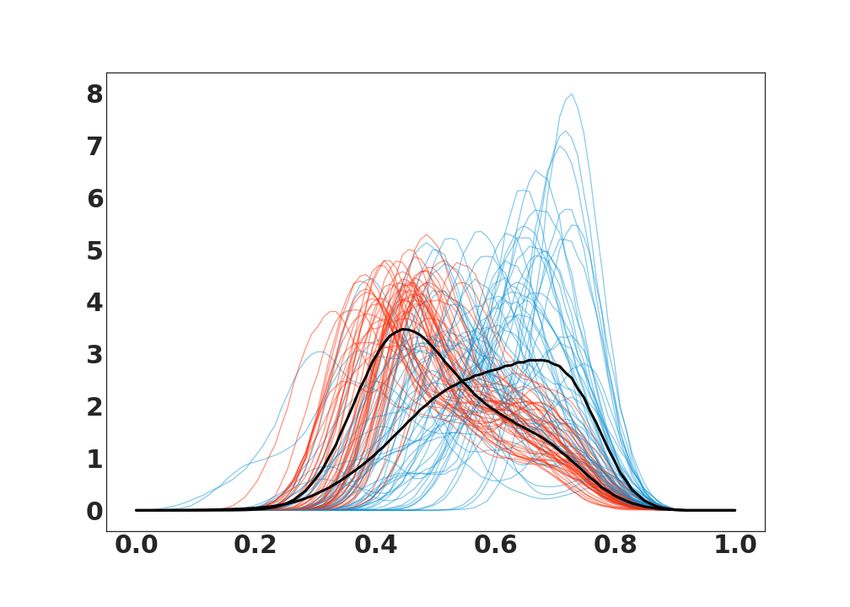
log-Euclidean, Jensen-Shannon and Wasserstein distances [43, 21, 39, 30, 7]. In this work, we extend
this formulation to PDFs space P with the Matérn covariance functions.
There is a rich literature on statistical inference on manifolds among which the Fisher information
matrix [35] has played a central role. Recently, there has been increasing interest in applying
information geometry for machine learning and data mining tasks [3, 6, 2, 8]. The Fisher information
matrix determines a Riemannian structure on a parametrized space of probability measures. Study
of geometry of P with the Riemannian structure, which we call information geometry, contributes
greatly to statistical inference, refer to [6, 2] for more details. Such methods are based on parametric
models that are of great interest in many applications. However, aspects of PDFs other than
parametric families may be important in various contexts [30, 25, 43, 40, 39? ]. In particular,
the consistency of regression and classification with PDFs inputs was established in [46, 31, 33]
with the help of kernel density estimation [12]. More recently, [7] studied the dissimilarity between
PDFs with the Wasserstein distance and [47] used a nonparametric framework to compare spherical
populations.
The main aim of this paper is to learn a Bayesian inference on Gaussian processes. For instance,
one can think of a Gaussian process as defining PDFs and inference taking place directly in the
function-space. Moreover, the index space is that of PDFs when choosing the underlying metric in
order to evaluate the dissimilarity between them [5]. The only drawback is that performing Kriging
on PDFs space P is not straightforward due to its geometry. For this end, we exploit an isometric
embedding by combinng the square root transform [11] and the distance induced by the Fisher-Rao
metric which make the covariance function non-degenerate and simplify the optimization process.
Gaussian processes (GPs) have been widely used to provide a probabilistic framework for a large
variety of machine learning methods [37]. Optimization techniques are usually required to fit a GP
model Z, that is to select a GP covariance function. For pi and pj in P, the main issue would be
to build a proper covariance between Z(pi ) and Z(pj ). In particular, this covariance can define a
notion of stationarity for the process. Another important task is the classification process where
we wish to assign an input PDF pi to one of the given classes [20].
To search for the covariance function hyperparameter, we use several methods for maximizing the
marginal likelihood. Our aim is then to select those optimizing performance criteria for regression
and classification: The first method is based on the gradient descent for finding a local maximum of
the marginal likelihood. The second method is a special case of MCMC methods, called Hamiltonian
Monte-Carlo (HMC) [15]. The objective is to perform sampling from a probability distribution for
which the marginal likelihood and its gradient are known. The latter has the advantage to simulate
from a physical system governed by Hamiltonian dynamics.
The remainder of the paper is organized as follows. In Section 2, we introduce the problem formu-
lation and we give a background of some Riemannian representations. Section 3 extends the usual
notion of GPs indexed by finite vectors to those indexed by PDFs with theoretical results for the
Matérn covariance function. We also give details of the proposed model for predicting and classi-
fying PDFs as well as estimating the covariance function parameters. In Section 4, we present and
discuss experimental results with some comparison studies. We conclude the paper in Section 5.

                                                   2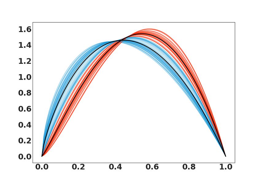
2. Problem formulation and geometry background

Let p1 , . . . , pn denote a finite set of observed PDFs and y1 , . . . , yn denote their corresponding outputs
with real values (quantitative or qualitative). In this work, we focus on nonparametric PDFs
restricted to be defined on Ω = [0, 1]. Our main goals throughout this paper are: i) Fitting the
proposed model’s parameters in order to better explain the link between pi and yi , i = 1, . . . , n,
ii) evaluating the corresponding predictive expectation at an unobserved PDF p∗ ∈ P and iii)
studying the properties of the GP with the Matérn covariance function. In the particular case where
yi ∈ {−1, +1}, we will assign each unobserved PDF p∗ to its predicted class after learning the model
parameters. To reach such goal, we follow the same idea of nonparametric information geometry
that has been discovered by [35] and developed later in other works, see for example [16, 43, 21, 6, 41].
Thus, the notion of similarity/dissimilarity between any pi and pj is measured using the induced
Rao distance [36, 5] between them on the underlying space. In this paper, we look at the space of
PDFs as a Riemannian manifold, as detailed in the next section, which plays an important role in
the proposed methods.

2.1. Riemannian structure of PDFs space
For more details about the geometric structure concerning the Fisher information metric, refer
to [16, 40, 9]. For example, [16] showed that P with a Riemannian structure has a positive constant
curvature. Furthermore, the action of orientation preserving diffeomorphism acts by isometry on
P with respect to the Fisher information metric. We will exploit these nice properties to define an
isometric embedding from P to E detailed in (11). Then, we use this embedding to construct a
Gaussian process on PDFs with a proper covariance function (14) and a predictive model (31).
We first note that the space of PDFs defined over Ω with values in R+ can be viewed in different
manners. The case where Ω is finite and the statistical model is parametric has been largely studied
in the literature [2, 6]. In contrast, if Ω is infinite which is the case here, different modeling options
have been explored [16, 32, 44, 9]. We start with the ideas developed in [16, 40, 43, 6] where P is an
infinite dimensional smooth manifold. That is, P is the space of probability measures that satisfy
the normalization constraint. Since we are interested in statistical PDFs analysis on P, we need
some geometrical tools [19, 24],e.g. geodesic. For the rest of the paper, we view P as a smooth
manifold (1) and we impose a Riemannian structure on it with the Fisher-Rao metric (3). Let
                                                           Z
                             P = {p : Ω → R | p ≥ 0 and       p(t)dt = 1}.                             (1)
                                                             Ω

be the space of all PDFs (positive almost everywhere) including nonparametric models. We identify
any tangent space of P, locally at each p, by
                                                      Z
                                Tp (P) = {f : Ω → R |    f = 0}                               (2)
                                                             Ω

As detailed in [13, 16, 9], the tangent space contains functions that are infinitesimally differentiable.
But following [19], we have a constructive method of great importance that allows one to form a
local version of any arbitrary f that is continuously differentiable in a small neighborhood and null
outside. Now that we have a smooth manifold and its tangent space, we can introduce a Riemannian
metric. This choice is very important since it will determine the structure of P and consequently the
covariance function of the Gaussian process. More details about the importance of the metric and
the induced Riemannian structure are discussed in [21, 38, 10]. We also define and denote by P+

                                                      3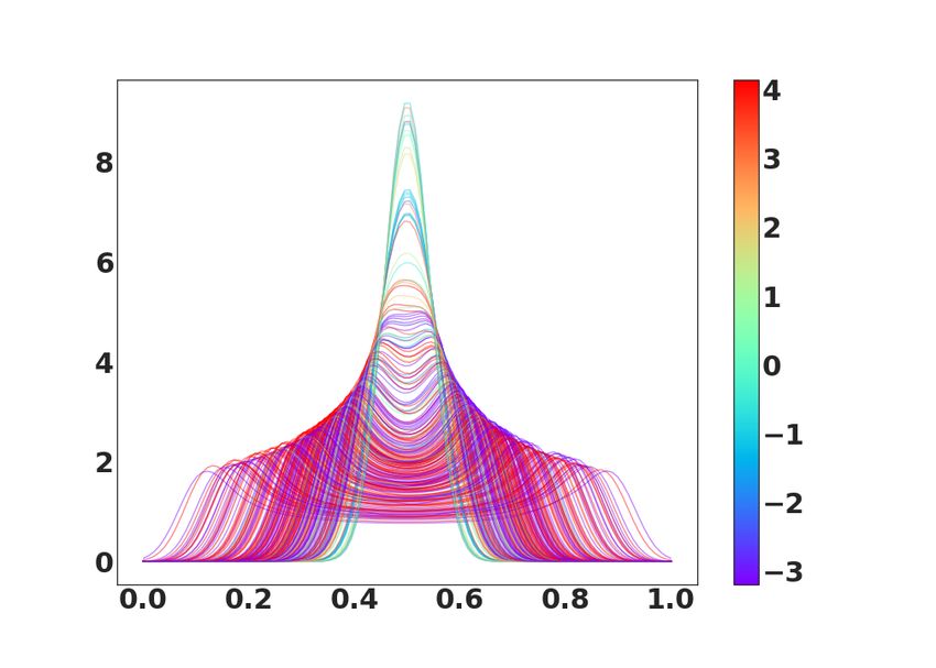
the interior of P. For the following, we consider without justification that any probability density
can be locally perturbed to be smooth enough [19]. This is true in finite dimensional cases but the
generalization to infinite dimensional cases is not straightforward. Among several metrics, we are
particularly interested in the Fisher-Rao metric defined, for any tangent vectors f1 , f2 ∈ Tp (P), by
                                                 Z
                                                    f1 (t)f2 (t)
                                  < f1 , f2 >p =                 dt.                               (3)
                                                  Ω     p(t)
Although this metric has nice properties with an increasing interest [40, 3, 13], P equipped with
< ., . >p is still numerically intractable. Therefore, instead of working on P directly, we consider
a mapping from P to the Hilbert upper-hemisphere (positive part) around the unity 1P such that
1P (t) = 1 for all t in Ω [11]. Thus, we exploit the Riemannian isometry between P and the
upper-hemisphere to extend the notion of GPs to the space of PDFs. Indeed, we first define the
map

                               Ψ:P     →   H                                                       (4)
                                                √                     1
                                   p   7 → φ = 2 p,     (p = Ψ−1 (φ) = φ2 )
                                                                      4
where
                                                          Z
                             H = {φ : Ω → R | φ ≥ 0 and       φ(t)2 dt = 4}.                       (5)
                                                          Ω

Note that φ is well defined since p is nonnegative and Ψ is a Riemannian isometry from P+ to H
without the boundary [24]. On the other hand, any element φ ∈ H can be uniquely projected as 12 φ
to have a unit norm. For simplicity and without loss of generality, we interpret H as the elements
                                     ∞
of unit Hilbert upper-hemisphere S+     up to a multiplicative factor (2 here). From that point of
                            ∞
view, we identify H with S+ and we define Ψ(1P ) = 1H to be the   √ ”unity pole” on H. Note that
1H as the image of the uniform pdf 1P is a fixed point, i.e. 1H = 1P = 1P . In this setup, we have
                                            Z
                                    kφk22 =    φ(t)2 dt = 1,                                   (6)
                                                Ω

for any φ in H which allow us to consider H, when equipped with the integral inner product < ., . >2 ,
as the unit upper-hemisphere (positive part). Furthermore, for arbitrary directions f1 , f2 in Tp (P)
the Fisher-Rao metric as defined in (eq:Fisher-Rao) becomes < ., . >2 as follows:

                                  < f1 , f2 >p =< Df1 Ψ, Df1 Ψ >2 .                                (7)
                   fi (t)
with Dfi Ψ(p)(t) = √      for all t ∈ Ω and i = 1, 2. One of the main advantages of this formulation is
                      p(t)
to exploit the nice properties of the unit Hilbert sphere such as geodesic, exponential map, log map,
and the parallel transport. For the rest of the paper, the geodesic distance dP (p1 , p2 ) between two
PDFs p1 and p2 in P, under the Fisher-Rao metric, is given by the geodesic distance dH (φ1 , φ2 ) (up
to a factor 2) between their corresponding φ1 and φ2 on H. We remind that the arc-length (geodesic
distance) between distinct and non antipodal φ1 and φ2 on H is the angle β = arccos (< φ1 , φ2 >2 ).
We also remind some geometric tools that will be needed for next sections as a lemma:
Lemma 2.1. With H defined from (5) with unit norm and Tφ (H) its tangent space at φ, we have
the following:

                                                    4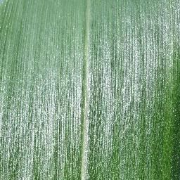
• The exponential map is a bijective isometry from the tangent space Tφ (H) to H. For any
     w ∈ Tφ (H), we write
                                                                             w
                                Expφ (w) = cos(kwk2 )φ + sin(kwk2 )              .                       (8)
                                                                            kwk2

   • Its inverse, the log map is defined from H to Tφ1 (H) as

                                                      β
                                   Logφ1 (φ2 ) =          (φ2 − cos(β)φ1 ).                              (9)
                                                   sin(β)

   • For any two elements φ1 and φ2 on H the map Γ : Tφ1 (H) → Tφ2 (H) parallel transports a
     vector w from φ1 to φ2 and is given by:

                                                       (φ1 + φ2 )
                               Γφ1 φ2 (w) = w − 2                   < w, φ2 >2                         (10)
                                                      ||φ1 + φ2 ||22

For more details, we refer to [24]. As a special case, we consider the unity pole φ = 1H and we
denote E = T1 (H) the tangent space of H at 1H . For simplicity, we note Log1 (.) the log map
from H to E and Exp1 (.) its inverse. This choice is motivated by two reasons: The numerical
implementation and the fact that 1H is the center of the geodesic disc [0, π2 [. Indeed and since all
elements are on the positive part, the exponential map and its inverse are diffeomorphisms. So,
one can consider any point on H instead of 1H to define the tangent space, e.g. the Fréchet mean.
However, this is without loss for the numerical precision. Furthermore we can use the properties of
the log map to show that:
                                                                           1
                          ||Log1 (φi ) − Log1 (φj )||2 = dH (φi , φj ) =     dP (pi , pj )              (11)
                                                                           2
for any two pi , pj on P. Note that the multiplicative factor 12 is important to guarantee the
isometry but will not have any impact on the covariance function defined in (14) as it is implicit in
the hyperparameter.

3. Gaussian Processes on PDFs

In this section, we focus on constructing GPs on P. A GP Z on P is a random field indexed by P
so that (Z(p1 ), . . . , Z(pn )) is a multivariate Gaussian vector for any n ∈ N\{0} and p1 , . . . , pn ∈ P.
A GP is completely specified by its mean function and its covariance function. We define a mean
function m : P → R and the covariance function C : P × P → R of a real process Z as

                                   m(pi ) =E Z(pi ) .                                                    (12)

                                C(pi , pj ) =E (Z(pi ) − m(pi ))(Z(pj ) − m(pj )) .                      (13)

Thus, if a GP is assumed to have zero mean function (m ≡ 0), defining the covariance function
completely defines the process behavior. In this paper, we assume that the GPs are centered and
we only focus on the issue of constructing a proper covariance function C on P.

                                                       5
3.1. Constructing covariance functions on P
A covariance function C on P must satisfy the following conditions. For any n ∈ N\{0} and
p1 , . . . , pn ∈ P, the matrix C = [C(pi , pj )]ni,j=1 is symmetric nonnegative definite. Furthermore, C
is called non-degenerate when the above matrix is invertible whenever p1 , . . . , pn are two-by-two
distinct [7]. The strategy that we adopt to construct covariance functions is to exploit the full
isometry map Log1 (.) to E given in (11). That is, we construct covariance functions of the form

                                C(pi , pj ) = K(kLog1 (φi ) − Log1 (φj )k2 ),                           (14)

where K : R+ → R.
Proposition 1. Let K : R+ → R be such that K(ui , uj ) = K(kui − uj k2 ) is a covariance function
on E and C as defined as in (14). Then
  1. C is a covariance function.
  2. If [K(kui − uj k2 )]ni,j=1 is invertible, then C is non-degenerate.
A closely related proof when dealing with Cumulative Density Functions (CDFs) is given in [7]. In
practice, we can select the function K from the Matérn family, letting for t ≥ 0

                                        δ2     2√νt ν  2√νt
                            Kθ (t) =                   Kν          ,                        (15)
                                     Γ(ν)2ν−1    α           α

where Kν is a modified Bessel function of the second kind and Γ is the gamma function. We
note θ = (δ 2 , α, ν) ∈ Θ where δ 2 > 0 is the variance parameter, α > 0 is the correlation length
parameter and ν = 12 + k(k ∈ N) is the smoothness parameter. The Matérn form [45] has the
desirable property that GPs have realizations (sample paths) that are k times differentiable [18],
which prove its smoothness as function of ν. As ν → ∞, the Matérn covariance function approaches
the squared exponential form, whose realizations are infinitely differentiable. For ν = 12 , the
Matérn takes the exponential form. From Proposition 1, the Matérn covariance function defined
by C(pi , pj ) = Kθ (kLog1 (φi ) − Log1 (φj )k2 ) is indeed non-degenerate.

3.2. Regression on P
Having set out the conditions on the covariance function, we can define the regression model on P
by

                                   yi = Z(pi ) + i , i = 1, . . . , n,                                 (16)

where Z is a zero mean GP indexed by P with a covariance function in the set {Cθ ; θ ∈ Θ}
        iid
and i ∼ N (0, γ 2 ). Here γ 2 is the observation noise variance, that we suppose to be known for
simplicity. Moreover, we note y = (y1 , . . . , yn )T , p = (p1 , . . . , pn )T and v = (v1 , . . . , vn )T =
(Log1 (Ψ(p1 )), . . . , Log1 (Ψ(pn )))T . The likelihood term is P(y|Z(p)) = N (Z(p), γ 2 In ) where In is
the identity matrix. Moreover, the prior on Z(p) is P(Z(p)) = N (0, Cθ ) with Cθ = [Kθ (kvi −
vj k2 )]ni,j=1 . We use the product of likelihood and prior terms to perform the integration yielding
the log-marginal likelihood
                                                                             n
                    lr (θ) = −yT (Cθ + γ 2 In )−1 y − log |Cθ + γ 2 In | −     log 2π.                  (17)
                                                                             2

                                                       6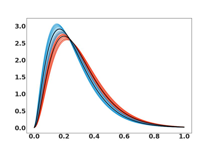
Let θ = {θj }3j=1 = (δ 2 , α, ν) denote the parameters of the Matérn covariance function Kθ . The
partial derivatives of lr (θ) with respect to θj are

                           ∂lr (θ)  1       ∂Cθ −1             ∂Cθ
                                   = yT C−1      Cθ y − tr C−1

                                j        θ     j            θ        .                           (18)
                            ∂θ      2       ∂θ                 ∂θj
For an unobserved PDF p∗ and by deriving the conditional distribution, we arrive at the key
predictive equation

                              P(Z(p∗ )|p, y, p∗ ) = N (µ(p∗ ), σ 2 (p∗ )),                       (19)

with
                                    µ(p∗ ) = C∗θ T (Cθ + γ 2 In )−1 y,
                               (
                                                                                                 (20)
                                   σ 2 (p∗ ) = Cθ∗∗ − C∗θ T (Cθ + γ 2 In )−1 C∗θ ,
where C∗θ = Kθ (v, v ∗ ) and Cθ∗∗ = Kθ (v ∗ , v ∗ ) for v ∗ = Log1 (Ψ(p∗ )). As we have introduced GP
regression indexed by PDFs, we will present GP classifier in the next section.

3.3. Classification on P
For the classification part, we focus on the case of binary outputs, i.e., yi ∈ {−1, +1}. We first
adapt the Laplace approximation to GPc indexed by PDFs in Section 3.3.1. We also give the
approximate marginal likelihood and the Gaussian predictive distribution in Section 3.3.2.

3.3.1. Approximation of the posterior
                                                                    Qn
The likelihood is the product of individual likelihoods P(y|Z(p)) = i=1 P(yi |Z(pi )) where P(yi |Z(pi )) =
                                                                           1
σ(yi Z(pi )) and σ(.) refers to the sigmoid function satisfying σ(t) = 1+exp(−t) . As for regression,
the prior law of GPc is P(Z(p)) = N (0, Cθ ). From the Bayes’ rule, the posterior distribution of
Z(p) satisfies

                                P(y|Z(p)) × P(Z(p))
                 P(Z(p)|y) =                        , ∝ P(y|Z(p)) × P(Z(p)),                     (21)
                                     P(y|p, θ)

where P(y|p, θ) is the exact marginal likelihood. The log-posterior is simply proportional to
log P(y|Z(p)) − 21 Z(p)T C−1
                           θ Z(p). For the Laplace approximation, we approximate the posterior
given in (21) by a Gaussian distribution. We can find the maximum a posterior (MAP) estimator
denoted by Ẑ(p), iteratively, according to

                     Z k+1 (p) = (Cθ + W)−1 (WZ k (p) + ∇P(y|Z k (p))),                          (22)

                                                         exp(−Ẑ(pi ))
where W is a n × n diagonal matrix with entries Wii = (1+exp(− Ẑ(pi )))2
                                                                          . Using the MAP estimator,
we can specify the Laplace approximation of the posterior by

                             P̂(Z(p)|p, y) = N (Ẑ(p), (C−1
                                                         θ + W)
                                                               −1
                                                                  ).                             (23)

                                                        7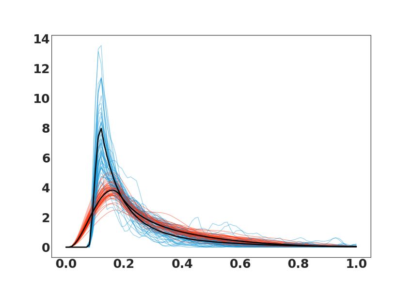
3.3.2. Predictive distribution
We evaluate the approximate marginal likelihood denoted by P̂(y|p, θ) instead of the exact marginal
likelihood P(y|p, θ) given in the denominator of (21). Integrating out Z(p), the log-marginal
likelihood is approximated by
                      1                                   1            1      1
            lc (θ) = − Ẑ(p)T C−1
                               θ Ẑ(p) + log p(y|Ẑ(p)) −   log In + W 2 Cθ W 2 .              (24)
                      2                                   2
The partial derivatives of lc (θ) with respect to θj satisfy
                                                  n
                            ∂lc (θ)   ∂lc (θ)     X  ∂lc (θ) ∂ Ẑ(pi )
                                    =         | +                      .                       (25)
                             ∂θj       ∂θj Ẑ(p) i=1 ∂ Ẑ(pi ) ∂θj

The first term, obtained when we assume that Ẑ(p) (as well as W) does not depend on θ, satisfies

             ∂lc (θ)     1     T    ∂Cθ −1      1               ∂Cθ
                     |  = Ẑ(p) C−1
                                 θ     C Ẑ(p) − tr (Cθ + W−1 )−1 j .                          (26)
              ∂θj Ẑ(p)  2          ∂θj θ       2                ∂θ

The second term, obtained when we suppose that only Ẑ(p) (as well as W) depends on θ, is
determined by

                        ∂lc (θ)          1  −1        ∂ 3 log p(y|Ẑ(p))
                                    =−      (Cθ + W)−1 ii                  ,                   (27)
                        ∂ Ẑ(pi )        2                    ∂ 3 Ẑ(pi )

and

                         ∂ Ẑ(p)              −1 ∂Cθ
                                 = I n + Cθ W         ∇ log p(y|Ẑ(p)).                        (28)
                           ∂θj                    ∂θj
Given an unobserved PDF p∗ , the predictive distribution at Z(p∗ ) is given by

                               P̂(Z(p∗ )|p, y, p∗ ) = N (µ(p∗ ), σ 2 (p∗ )),                   (29)

with
                                     µ(p∗ ) = C∗θ T C−1
                               (
                                                     θ Ẑ(p),
                                                                                               (30)
                                    σ 2 (p∗ ) = Cθ∗∗ − C∗θ T (Cθ + W−1 )−1 C∗θ .
Finally, using the moments of prediction, the predictor for y ∗ = +1 is
                                     Z
                            π(p∗ ) =    σ(Z ∗ )P̂(Z ∗ |p, y, p∗ )dZ ∗ ,                        (31)
                                             R

where we note Z ∗ = Z(p∗ ) for simplicity.

3.4. Covariance parameters estimation
The marginal likelihoods for both regression and classification depend on the covariance parameters
controlling the stationarity of the GP. To show potential applications of this framework, we explore
several optimization methods in Section 3.4.1 and Section 3.4.2.

                                                        8
3.4.1. log-marginal likelihood gradient
In the marginal likelihood estimation, the parameters are obtained by maximizing the log-marginal
likelihood with respect to θ, i.e., finding
θ̂ = argmax ll (θ), (32)
θ
where ll (θ) is given in (17) by lr (θ) for regression or lc (θ) in( 24) for classification. We summarize
the main steps in Algorithm 1.
Algorithm 1: Gradient descent.
Require: log-marginal likelihood ll and its gradient ∇ll
Ensure: θ̂
1: repeat
2: ∇ll (θ(k)) = { ∂ll∂θ
(θ(k)) 3
j }j=1 from (18) or (25)
3: Find the step-size λ (e.g., by backtracking line search)
4: Evaluate θ(k + 1) = θ(k) − λ∇ll (θ(k))
5: Set k = k + 1
6: until ||∇ll ||2 is small enough or a maximum iterations is reached
3.4.2. HMC sampling
Generally, the marginal likelihoods are non-convex functions. Indeed, conventional optimization
routines may not find the most probable candidate leading to a lost of robustness and uncertainty
quantification. To deal with such limitations, we use weak prior distributions for δ 2 and α whereas
ν is simply estimated by cross-validation [28]:
P(δ 2 , α) = P(δ 2 ) × P(α), (33)
with δ 2 and α being independent. Following [17], δ 2 will be assigned a half-Cauchy (positive-only)
prior, i.e. P(δ 2 ) = C(0, bδ2 ) and α an inverse gamma, i.e. P(α) = IG(aα , bα ). Consequently, the
log-marginal posterior is proportional to
lp (δ 2 , α) = ll (θ) + log P(δ 2 ) + log P(α). (34)
When sampling from continuous variables, HMC can prove to be a more powerful tool than usual
MCMC sampling. We define the Hamiltonian as the sum of a potential energy and a kinetic energy:
2
1 X j2
E((θ1 , θ2 ), (s1 , s2 )) = E 1 (θ1 , θ2 ) + E 2 (s1 , s2 ) − lp (θ1 , θ2 ) + s , (35)
2 j=1
which means that (s1 , s2 ) ∼ N (0, I2 ). Instead of sampling from exp lp (θ1 , θ2 ) directly, HMC
operates by sampling from the distribution exp − E((θ1 , θ2 ), (s1 , s2 )) . The differential equations
are given by
dθj ∂E dsj ∂E ∂E 1
= j = sj and =− j =− j , (36)
dt ∂s dt ∂θ ∂θ
9for j = 1, 2. In practice, we can not simulate Hamiltonian dynamics exactly because of time
discretization. To maintain invariance of the Markov chain, however, care must be taken to preserve
the properties of volume conservation and time reversibility. The leap-frog algorithm, summarized
in Algorithm 2, maintains these properties [29].
Algorithm 2: Leap-frog.
1: for k = 1, 2, . . . do
2: sj (k + λ2 ) = sj (k) − λ2 ∂θ∂ j E 1 (θ1 (k), θ2 (k)) where λ is a finite step-size
3: θj (k + λ) = θj (k) + λsj (k + λ2 )
4: sj (k + λ) = sj (k + λ2 ) − λ2 ∂θ∂ j E 1 (θ1 (k + λ), θ2 (k + λ))
5: end for
We thus perform a half-step update of the velocity at time k + λ2 , which is then used to compute
θj (k + λ) and sj (k + λ). A new state ((θ1 (N ), θ2 (N )), (s1 (N ), s2 (N ))) is then accepted with the
probability
exp − E((θ1 (N ), θ2 (N ), (s1 (N ), s2 (N ))
min 1, . (37)
exp − E((θ1 (1), θ2 (1), (s1 (1), s2 (1))
We summarize the HMC sampling in Algorithm 3.
Algorithm 3: HMC sampling.
Require: log-marginal posteriors lp and its gradient ∇lp
Ensure: θ̂
1: Sample a new velocity from a Gaussian distribution (s1 (1), s2 (1)) ∼ N (0, I2 )
2: Perform N leapfrog steps to obtain the new state (θ 1 (N ), θ 2 (N )) and velocity (s1 (N ), s2 (N ))
from Algorithm 2
3: Perform accept/reject of (θ 1 (N ), θ 2 (N )) with acceptance probability defined in (37).
4. Experimental Results
In this section, we test and illustrate the proposed methods using synthetic, semi-synthetic and real
data. For all experiments, we study the empirical results of a Gaussian process indexed by PDFs
for both regression and classification.
Baselines. We compare results of GP indexed by PDFs (GPP) where the parameters are estimated
by gradient descend (G-GPP) and HMC (HMC-GPP) to: Functional Linear Model (FLM) [34] for
regression, Nonparametric Kernel Wasserstein (NKW) [42] for regression, A GPP based on the
Wasserstein distance (W-GPP) [27, 7] for classification, and a GPP based on the Jensen-Shannon
divergence (JS-GPP) [30] for classification.
Performance metrics. For regression, we illustrate the performance of the proposed framework
in terms of root mean square error (RMSE) and negative log-marginal likelihood (NLML). For
classification, we consider accuracy, area under curve (AUC) and NLML.
10Figure 1: Examples of PDFs input for regression. The output with continuous value in [−3, 4] is illustrated by a
colorbar.
4.1. Regression
Dataset. We first consider a synthetic dataset where we observe√a finite set of functions simulated
√ √ √
according to (16) as Z(pi ) = h(< pi , p̃ >2 ) = 0.5 < pi , p̃ >2 +0.5. In this example, we
consider a truncated Fourier basis √ (TFB) with random √ Gaussian coefficients to form the original
functions satisfying
√ gi (t) = δ √
i,1 2 sin(2πt) + δ i,2 2 cos(2πt) with δi,1 , δi,2 ∼ N (0, 1). We also take
g̃(t) = −0.5 2 sin(2πt) + 0.5 2 cos(2πt). We suppose that p̃ and pi s refer to the corresponding
PDFs of g̃ and gi s estimated from samples using the nonparametric kernel method (bandwidths
were selected using the method given in [12]). Examples of n = 100 estimates are displayed in
Fig. 1 with colors depending on their output levels.
Regression results. Focusing on RMSE, we summarize all results in Table 1. Accordingly, the
proposed G-GPP gives better precision than FLM. On the other hand, HMC-GPP substantially
outperforms NKW with a significant margin. As illustrated in Table 2, we note that the proposed
methods are more efficient than the baseline FLM when maximizing the log-marginal likelihood.
Again, this is a very simple explanation on how the quality of GPP strongly depends on parameters
estimation method. In addition, G-GPP stated in Algorithm 1 is very effective from a computational
point of view.
Table 1: Regression: RMSE as a performance metric.
G-GPP HMC-GPP FLM NKW
mean std mean std mean std mean std
0.07 0.03 0.13 0.31 0.10 0.04 0.28 0.01
Table 2: Regression: negative log-marginal likelihood as a performance metric.
G-GPP HMC-GPP FLM
mean std mean std mean std
73.28 1.14 21.89 5.32 329.66 6.52
114.2. Classification
In this section, we perform some extensive experiments to evaluate the proposed methods using a
second category of datasets.
4.2.1. Datasets for classification
Synthetic datasets. We consider a dataset of two synthetic PDFs of beta and inverse gamma
distributions. This choice is very crucial for many reasons since beta is defined on [0, 1], parametrized
by two positive parameters, and has been widely used to represent a large family of PDFs with finite
support in various fields. Increasingly, the inverse gamma plays an important role to characterize
random fluctuations affecting wireless channels [4]. In both examples, the covariance matrix with L2
distance and Total Variation TV-distance have a very low rank. We performed this experiment by
simulating n = 200 pairs of PDFs slightly different for the two classes. Each observation represents
a density when we add a random white noise. We refer to these datasets as Beta and InvGamma,
see random examples in Fig. 2 (a&b). We also illustrate the Fréchet mean for each class. The
search of the mean is performed using a gradient approach detailed in [43].
Semi-synthetic dataset. Data represent clinical growth charts for children from 2 to 12 years [34].
We refer to this dataset as Growth. We simulate the charts from centers for disease control and
prevention [22] through the available quantile values. The main goal is to classify observations by
gender. Each simulation represents the size growth (the increase) of a child according to his age
(120 months). We represent observations as nonparametric PDF and we display some examples in
Fig. 2 (c). For each class: girls (red) and boys (blue) we show the Fréchet mean in black.
Real dataset. The first public dataset consists of 1500 images representing maize leaves [14] with
specific textures whereas the goal is to distinguish healthy and non-healthy plants. We refer to this
dataset as Plants. Motivated by this application, we first represent each image with its wavelet-
deconvolved version and form a high-dimensional vector of 262144 components. Fig. 3 illustrates
an example of two original images (left): a healthy plant (top) and a plant with disease (bottom),
their wavelet-deconvolved versions (middle), and the corresponding histograms (right). We also
display PDFs from histograms for each example in Fig. 3 (right column in black).
A second real dataset with 1717 observations gives the body temperature of dogs. For this dataset,
temporal measures of infected and uninfected dogs are stored during 24 hours. The infection by a
parasite is suspected to cause persistent fever despite veterinary medicine [23]. The main goal is to
learn the relationship between the infection and a dominant pattern from temporal temperatures.
We display some examples of infected (blue) and uninfected (red) in Fig. 2 (c) and we refer to
this dataset as Temp. The PDF estimates were obtained using an automatic bandwidth selection
method described in [12]. We illustrate some examples of PDFs from real datasets in Fig. 2 (d&e).
We remind that high-dimensional inputs make traditional machine learning techniques fail to solve
the problem at hand. However, the spectral histograms as marginal distributions of the wavelet-
deconvolved image can be used to represent/classify original images [26]. In fact, instead of com-
paring the histograms, a better way to compare two images (here a set of repetitive features) would
be to compare their corresponding densities.
4.2.2. Classification results
We learn the model parameters from 75% of the dataset whereas the rest is kept for test. This
subdivision has been performed randomly 100 times. The performance is given as a mean and the
corresponding standard deviation (std) in order to reduce the bias (class imbalance and sample
12(a) (b)
(c) (d) (e)
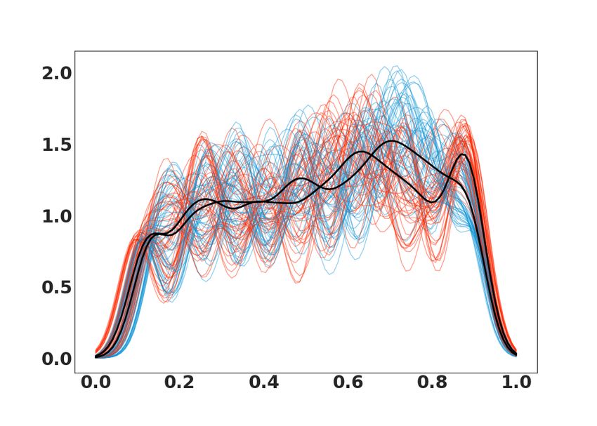
Figure 2: Synthetic PDFs for (a) InvGamma and (b) Beta with class 1 (red) and class 2 (blue). Semi-synthetic
PDFs for (c) Growth with girls (red) and boys (blue). Real PDFs for (d) Temp with uninfected (red) and infected
(blue). Real PDFs for (e) Plants with disease (red) and healthy (blue). The Fréchet mean for each class in black.
Figure 3: Two examples from maize plants dataset where (top) is a healthy leaf and (bottom) is a leaf with disease.
For each class: an original image (left), the extracted features (middle), and the normalized histogram (right).
representativeness) introduced by the random train/test split.
Results on synthetic datasets. We summarize all evaluation results on synthetic datasets
in Fig. 4 (a&b). Accordingly, one can observe that both HMC-GPP, W-GPP and JS-GPP reach
the best accuracy values for InvGamma with a little margin for the proposed HMC-GPP. On the
other hand, G-GPP and HMC-GPP heavily outperform W-GPP and JS-GPP for Beta. Again, this
13(a)
(b)
(c)
Figure 4: Boxplots of the classification accuracy (left) and AUC (right) on synthetic and semi-synthetic datasets:
(a) InvGamma, (b) Beta, and (c) Growth. In each subfigure, the performance is given for different methods: G-GPP
(red), HMC-GPP (light blue), W-GPP (violet), and JS-GPP (dark blue).
simply shows how each optimization method impacts the quality of the predictive distributions.
Results on semi-synthetic data. We summarize all results in Fig. 4 (c) where we show accuracy
and AUC values on the Growth dataset as boxplots from 100 tests. One can observe that G-GPP
gives the best accuracy with a significant margin. Note that we have used 103 HMC iterations
in Algorithm 3. Furthermore, we set the “Burn-in” and “Thinning” in order to ensure a fast
convergence of the Markov chain and to reduce sample autocorrelations.
Results on real data. We further investigate whether our proposed methods can be used with
real data. Fig. 5 (a&b) shows the boxplots of accuracy and AUC values for Temp and Plants,
respectively. In short, we highlight that the proposed methods successfully modeled these datasets
with improved results in comparison with W-GPP.
14(a)
(b)
Figure 5: Boxplots of the classification accuracy (left) and AUC (right) on real datasets: (a) Temp and (b) Plants.
In each subfigure, the performance is given for different methods: G-GPP (red), HMC-GPP (light blue), W-GPP
(violet), and JS-GPP (dark blue).
Fortunately, the experiments have shown that the problem of big iterations, usually needed to
simulate the Markov chains for complex inputs is partially solved by considering the proposed HMC
sampling (Algorithm 3). In closing, we can state that the leap-frog algorithm (Algorithm 2), based
on Hamiltonian dynamics, allows us to early search the best directions giving the best minimum of
the Hamiltonian defined in (35).
4.2.3. Summary of all classification results
Table 3: Classification: negative log-marginal likelihood as a performance metric.
Datasets Synthetic Semi-synthetic Real data
InvGamma Beta Growth Temp Plants
Method mean std mean std mean std mean std mean std
G-GPP 30.50 2.43 4.41 0.06 68.03 3.43 98.66 0.73 98.65 0.72
HMC-GPP 105.35 0.22 105.28 0.21 61.65 2.24 105.36 0.22 9.33 0.21
JS-GPP 32.2 2.38 42.87 2.73 62.0 3.02 116.65 4.13 10.26 0.12
We also confirm all previous results from Table 3, which summarizes the mean and the std of NLML
values for all datasets. These clearly show that at least one of the proposed methods (G-GPP or
HMC-GPP) better minimizes the NLML than JS-GPP. This brings more quite accurate estimates,
which prove the predictive power of our approaches.
155. Conclusion
In this paper, we have introduced a novel framework to extend Bayesian learning models and Gaus-
sian processes when the index support is identified with the space of probability density functions
(PDFs). We have detailed and applied different numerical methods to learn regression and classifi-
cation models on PDFs. Furthermore, we showed new theoretical results for the Matérn covariance
function defined on the space of PDFs. Extensive experiments on multiple and varied datasets have
demonstrated the effectiveness and efficiency of the proposed methods in comparison with current
state-of-the-art methods.
Acknowledgements
This work was partially funded by the French National Centre for Scientific Research.
References
[1] M. Abt and W.J. Welch. Fisher information and maximum-likelihood estimation of covariance
parameters in Gaussian stochastic processes. The Canadian Journal of Statistics, 26:127–137,
1998.
[2] S.-I. Amari. Information geometry and its applications. Springer, Tokyo, Japan, 1st edition,
2016.
[3] S.-I. Amari, O.E. Barndorff-Nielsen, R.E. Kass, S.L. Lauritzen, and C.R. Rao. Differential
geometry in statistical inference. Institute of Mathematical Statistics, Hayward, CA, 1987.
[4] S. Atapattu, C. Tellambura, and H. Jiang. A mixture gamma distribution to model the snr of
wireless channels. IEEE Transactions on Wireless Communications, 10:4193–4203, 2011.
[5] C. Atkinson and A.F.S. Mitchell. Rao’s distance measure. The Indian Journal of Statistics,
43:345–365, 1981.
[6] N. Ay, J. Jost, H.V. Le, and L. Schwachhöfer. Information geometry. Springer, Cham, Switzer-
land, 2017.
[7] F. Bachoc, F. Gamboa, J-M. Loubes, and N. Venet. A Gaussian process regression model for
distribution inputs. IEEE Transactions on Information Theory, 64:6620–6637, 2018.
[8] Frédéric Barbaresco. Information Geometry of Covariance Matrix: Cartan-Siegel Homogeneous
Bounded Domains, Mostow/Berger Fibration and Fréchet Median, chapter 9, pages 199–255.
Springer, Berlin, Heidelberg, 2013.
[9] M. Bauer, M. Bruveris, and P.W. Michor. Uniqueness of the Fisher–Rao metric on the space
of smooth densities. Bulletin of the London Mathematical Society, 48:499–506, 2016.
[10] M. Bauer, E. Klassen, S.C. Preston, and Z. Su. A diffeomorphism-invariant metric on the
space of vector-valued one-forms, 2018.
[11] A. Bhattacharyya. On a measure of divergence between two statistical populations defined by
their probability distributions. Bulletin of the Calcutta Mathematical Society, 35:99–109, 1943.
16[12] Z.I. Botev, J.F. Grotowski, and D.P. Kroese. Kernel density estimation via diffusion. The
Annals of Statistics, 38:2916–2957, 2010.
[13] N.N. Cencov. Statistical decision rules and optimal inference. Translations of Mathematical
Monographs. American Mathematical Society, Providence, R.I., 1982.
[14] C. DeChant, T. Wiesner-Hanks, S. Chen, E. Stewart, J. Yosinski, M. Gore, R. Nelson, and
H. Lipson. Automated identification of northern leaf blight-infected Maize plants from field
imagery using deep learning. Phytopathology, 107:1426–1432, 2017.
[15] S. Duane, A. Kennedy, B. Pendleton, and D. Roweth. Hybrid Monte Carlo. Physics Letters
B, 195:216–222, 1987.
[16] T. Friedrich. Die Fisher-information und symplektische strukturen. Mathematische
Nachrichten, 153:273–296, 1991.
[17] A. Gelman. Prior distributions for variance parameters in hierarchical models. Bayesian
Analysis, 1:515–533, 2006.
[18] M.G. Genton and W. Kleiber. Cross-covariance functions for multivariate geostatistics. Sta-
tistical Science, 30:147–163, 2015.
[19] S. Helgason. Differential geometry, lie groups, and symmetric spaces. Academic Press, New
York, 1978.
[20] D. Hernández-Lobato, J.M. Hernández-lobato, and P. Dupont. Robust multi-class Gaussian
process classification. In Proceedings of the 24th International Conference on Neural Informa-
tion Processing Systems, NIPS’11, pages 280–288, Red Hook, NY, USA, 2011. Curran Asso-
ciates, Inc.
[21] M. Itoh and H. Satoh. Geometry of Fisher information metric and the barycenter map. Entropy,
17:1814–1849, 2015.
[22] R.J. Kuczmarski, C. Ogden, S.S. Guo, L. Grummer-Strawn, K.M. Flegal, Z. Mei, R. Wei,
L.R. Curtin, A.F. Roche, and C.L. Johnson. 2000 CDC growth charts for the united states:
methods and development. Vital and Health Statistics, 246:1–190, 2002.
[23] P. Kumar and A. Kumar. Haemato-biochemical changes in dogs infected with Babesiosis. In
Conference on Food Security and Sustainable Agriculture, pages 21–24. International Journal
of Chemical Studies, 2018.
[24] J.M. Lee. Riemannian manifolds: An introduction to curvature. Springer Science, New York,
1997.
[25] F. Nielsen and M. Liu and B.C. Vemuri. Jensen divergence-based means of SPD matrices,
chapter 6, pages 111–122. Springer, Berlin, Heidelberg, 2013.
[26] X. Liu and D. Wang. Texture classification using spectral histograms. IEEE Transactions on
Image Processing, 12:661–670, 2003.
17[27] A. Mallasto and A. Feragen. Learning from uncertain curves: the 2-Wasserstein metric for
Gaussian processes. In Neural Information Processing Systems (NIPS), pages 5660–5670. Cur-
ran Associates, Inc., Long Beach, CA, USA, 2017.
[28] R.M. Neal. Monte Carlo implementation of Gaussian process models for Bayesian regres-
sion and classification. Technical report. University of Toronto (Dept. of Statistics), Toronto,
Canada, 1997.
[29] R.M. Neal. MCMC using Hamiltonian dynamics. Handbook of Markov Chain Monte Carlo,
54:113–162, 2010.
[30] H.V. Nguyen and J. Vreeken. Non-parametric Jensen-Shannon divergence. In Machine Learn-
ing and Knowledge Discovery in Databases, pages 173–189, Cham, Switzerland, 2015. Springer
International Publishing.
[31] J.B. Oliva, W. Neiswanger, B. Póczos, J. G. Schneider, and E. P. Xing. Fast distribution to real
regression. In Proceedings of the Seventeenth International Conference on Artificial Intelligence
and Statistics, Proceedings of Machine Learning Research, pages 706–714, Reykjavik, Iceland,
2014. PMLR.
[32] G. Pistone and C. Sempi. An infinite-dimensional geometric structure on the space of all the
probability measures equivalent to a given one. The Annals of Statistics, 23:1543–1561, 1995.
[33] B. Póczos, A. Singh, A. Rinaldo, and L. Wasserman. Distribution-free distribution regres-
sion. In Proceedings of the Sixteenth International Conference on Artificial Intelligence and
Statistics, pages 507–515, Scottsdale, Arizona, USA, 2013. PMLR.
[34] J.O. Ramsay and B.W. Silverman. Functional Data Analysis. Springer-Verlag, New York,
USA, 2005.
[35] C.R. Rao. Information and the accuracy attainable in the estimation of statistical parameters.
Bulletin of Calcutta Mathematical Society, 37:81–91, 1945.
[36] C.R. Rao. Diversity and dissimilarity coefficients: A unified approach. Theoretical Population
Biology, 21:24–43, 1982.
[37] C.E. Rasmussen and C.K.I. Williams. Gaussian processes for machine learning. The MIT
Press, Cambridge, London, 2006.
[38] C. Samir, P.-A. Absil, A. Srivastava, and E. Klassen. A gradient-descent method for curve
fitting on Riemannian manifolds. Foundations of Computational Mathematics, 12:49–73, 2012.
[39] C. Samir, S. Kurtek, A. Srivastava, and N. Borges. An elastic functional data analysis frame-
work for preoperative evaluation of patients with rheumatoid arthritis. In Winter Conference
on Applications of Computer Vision, pages 1–8, Lake Placid, NY, USA, 2016. IEEE.
[40] Y. Shishido. Strong symplectic structures on spaces of probability measures with positive
density function. Proceedings of the Japan Academy, Series A, Mathematical Sciences, 81:134–
136, 2005.
[41] B. Sriperumbudur, K. Fukumizu, A. Gretton, A. Hyvärinen, and R. Kumar. Density estimation
in infinite dimensional exponential families, 2013.
18[42] B.K. Sriperumbudur, K. Fukumizu, A. Gretton, B. Schölkopf, and G.R.G. Lanckriet. Non-
parametric estimation of integral probability metrics. In International Symposium on Infor-
mation Theory (ISIT), pages 1428–1432, Piscataway, NJ, USA, 2010. IEEE.
[43] A. Srivastava, I. Jermyn, and S. Joshi. Riemannian analysis of probability density func-
tions with applications in vision. In Conference on Computer Vision and Pattern Recognition
(CVPR), pages 1–8, Minneapolis, USA, 2007. IEEE.
[44] A. Srivastava and E. Klassen. Functional and shape data analysis. Springer-Verlag, New York,
USA, 2016.
[45] M.L. Stein. Interpolation of spatial data. Springer-Verlag, New York, USA, 1999.
[46] D.J. Sutherland, J.B. Oliva, B. Póczos, and J.G. Schneider. Linear-time learning on distribu-
tions with approximate kernel embeddings. In Proceedings of the Thirtieth AAAI Conference
on Artificial Intelligence, AAAI’16, pages 2073–2079, Phoenix, Arizona, 2016. AAAI Press.
[47] Z. Zhang, E. Klassen, and A. Srivastava. Robust comparison of kernel densities on spherical
domains. Sankhya A: The Indian Journal of Statistics, 81:144–171, 2019.
19You can also read